Appl. Magn. Reson. 20, 137-150 (2001) Applied
Magnetic Resonance
© Springer-Verlag 2001
Printed in Austria
Measurement of Spin-Lattice Relaxation Times
with Longitudinal Detection
J. Granwehr and A. Schweiger
Physical Chemistry Laboratory, Swiss Federal Institute of Technology, Zurich, Switzerland Received January 9, 2001
Abstract. New experimental schemes to measure splattice relaxation times T, on the basis of in-version-recovery and saturation-recovery experiments with longitudinal detection are introduced. With this approach, paramagnetic species with Ti values as short as 20 ns can be measured. Possibilities
to reduce unwanted signals and instrumental artifacts are analyzed. An experiment where the signal is induced directly by the time-dependent M. magnetization is also proposed. Experimental results for organic radicals and defect centers are presented and compared with data obtained with conven-tional techniques, and a metal complex at 250 K is analyzed where it is very difficult to get infor-mation about relaxation times with established methods because of fast spin-spin relaxation.
1 Introduction
During the last five decades, a variety of different methods have been developed to determine the spin-lattice relaxation time T, of paramagnetic species. Among the most popular techniques are the inversion-recovery (IR) [1] and the satura-tion-recovery (SR) [2] experiments. The major drawback of these methods which measure transverse magnetization is that either an additional low-power pulse channel is required for probe-pulse detection or the spin-spin relaxation time TZ
has to be long enough to observe an electron spin echo. As an alternative, T, can be determined with longitudinal detection (LOD), where the change in the longitudinal
M
magnetization is recorded with a pickup coil. A variety of LOD-EPR methods have been proposed, as for example, saturation methods [3], the analysis of the signal induced by the return of M. to Boltzmann equilibrium ([4] and P. Hofer, pers. commun.), techniques where the detection frequency is var-ied [5], and pulse LOD-EPR schemes [6]. All these methods are deadtime free, but most of them suffer from a low sensitivity and require a dedicated instru-mental setup.Recent developments in instrumentation of pulse LOD-EPR on the basis of a commercially available spectrometer [7] now open new possibilities for the de-termination of Ti with high sensitivity. In this contribution we present pulse LOD
experiments, where the IR or SR preparation sequence is combined with a new detector sequence, and demonstrate the applicability of the methods for the di-rect measurement of short T, values (P. Hofer, pers. commun.). The study is focused on the realization and optimization of the experiments and on the data analysis. The potentials and limitations of the approaches are demonstrated for different types of samples. First, the methods are applied to samples such as a,a-diphenyl-(3-picrylhydrazyl (DPPH) and y-irradiated herasil glass, where T, can also be obtained with conventional techniques. Second, it is demonstrated that T, times of metal complexes at noncryogenic temperatures can be measured, which is usually not possible with methods using detection of the transverse magnetiza-tion because of the short T2 times. As an example, the relaxation processes of a
natural dolomite, where both Ca(II) and Mg(II) sites are substituted by Mn(II), are studied.
2 Theory
2.1 Inversion- and Saturation-Recovery Experiments
After excitation, the return of the longitudinal component of the magnetization to thermal equilibrium can often be described by [8]
M_(t) = M
eq+ [M^(0)
— Meq] exp ^ Til , (1)
where Meq is the magnetization at Boltzmann equilibrium, M(0) is the
longitu-dinal magnetization at the beginning of the relaxation process, and MM(t) is the
value of the z-magnetization at time t.
In an IR experiment, Meq is inverted with a it preparation pulse, and M(t) is read out with an appropriate detector sequence, usually a probe pulse or a two-pulse echo. In the case of echo detection, time T between inversion and detec-tion is increased step by step, and the recovery is recorded point by point, while with probe-pulse detection the recovery is recorded in one shot, resulting in a shorter measuring time. In an SR experiment, a saturation instead of an inver-sion pulse is applied at the beginning of the sequence.
The main problem with detection of the transverse magnetization is the de-pendence of the signal intensity on T2. In the case of probe-pulse detection, the
signal is proportional to
T
2 ifT, >> T
z and lIT2 >> a)„ where c , is theampli-tude of the microwave (mw) field in angular frequencies [9]. With the two-pulse echo detection sequence, TZ has to be longer than the instrumental deadtime. This
is usually the case for transition metal compounds at cryogenic temperatures and for radicals at ambient temperatures. At room temperature, transition metal com-plexes have very short T2 times, which makes it difficult or even impossible to
measure T, with standard techniques.
A different approach is to measure directly M(T). This can be achieved by changing the Mz magnetization at time T by a microwave (mw) pulse which in
T, Measurement with Longitudinal Detection 139
turn induces a voltage proportional to M(I) in a pickup coil oriented along the
Bo-field direction. The coil can be placed inside the mw resonator and is part of
a serial LCR resonant circuit with resonant frequency coLCR and quality factor QLCR. The time constant of the detection circuit is given by zLcR = 2QLCR/WLCR•
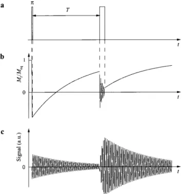
The relaxation behavior is measured in an analogous way as in an IR or SR ex-periment with echo detection by increasing time T step by step. The pulse scheme for the inversion-recovery longitudinally detected T, experiment (IR-LOD T1), the progression of M_, and the response of the detection circuit are shown in Fig. 1. The saturation-recovery longitudinally detected T, experiment (SR-LOD T1) is analogous, with the inversion pulse replaced by a saturation pulse. The signal in Fig. lc for t >_ T can be detected with a transient recorder. Instead of a tran-sient recorder, a boxcar averager can be used. To avoid a cancellation of the sig-nal by the averaging process of the boxcar, either the length of the boxcar win-dow has to be adjusted to a value tbox < TLcR/2 with the period TLCR = 27u/wt.cR
and the window has to be properly positioned, or the signal has to be rectified before data acquisition. With a boxcar averager, the amount of data is by orders of magnitude lower than those obtained with a transient recorder, since for each
T
t
b
C
in
Fig. 1. The IR-LOD T, experiment. a Pulse sequence consisting of an inverting it pulse followed by a free evolution period of time T during which the magnetization relaxes towards the Boltzmann equilibrium. At time T a nutation pulse is applied to read out M(T). b Progression of M as a func-tion of time t. In this simulafunc-tion a ratio between the longitudinal and the transverse relaxafunc-tion time of TJIT2 = 25 is used. c Simulated response of a serial LCR detection circuit with a quality factor
T value the data set representing the signal is reduced to a single point. If the signal is measured with a transient recorder, this reduction of the data is done after data acquisition [7]. One possibility is to calculate the amplitude of the spectral component at w,cR of the signal caused by the detection pulse. Another option is to sum up the absolute values of all data points after a baseline cor-rection. In the case of T, << TLcR, it might be preferable to sum up only the data points during the first half-period of the oscillating signal, which is equivalent to the use of a boxcar averager for detection.
The effect of the mw detection pulse on the magnetization depends also on T2. If Tz is long enough that the nutation of the magnetization during the pulse
lasts at least for one period TLcR, optimum sensitivity is obtained with a nuta-tion frequency w = LCR. If the decay of the magnetization can be refocused, the signal intensity can be further improved by periodically inverting the phase of the mw field. This results in a series of rotary echoes as in a TN-LOD EPR experiment [7]. For Tz << 2llcoTN„ the magnetization does not nutate, but a
sig-nal can still be observed because of the decay of MM during the pulse. It is there-fore possible to measure T, for very short values of T2.
For the two methods IR-LOD T, and SR-LOD T1, there exists a lower but
not an upper limit for T1. This is mainly caused by two reasons. First, the reso-lution of the transient recorder is limited. For a reasonable fit of the data, a few data points should be collected until Meq is reached. Second, because of the
fi-nite rise and fall time of the mw switches and the fifi-nite bandwidth Aco of the mw resonator, the edges of the pulses can no longer be considered as infinitely short, whenever the switching times or 2 tIAar are longer than T,. In this case the decay of the observed signal is determined by both the relaxation time T, and the time constant of the fall time of the preparation pulse. This effect can be reduced by reducing the switching times and by lowering the quality factor of the resonator. With our setup, T, values down to approximately 20 ns can be measured.
A signal is not only induced in the coil by the change of Mz during the
detection pulse but also during the inversion or saturation pulse (Fig. lc). Since in most experiments the detection pulse is applied before the signal induced by the preparation pulse has decayed, the observed time trace during and after the detection pulse is a superposition of both signals. Consequently, when time T is incremented in an IR-LOD T, or SR-LOD T, experiment, the relaxation curve is modulated with WLcR. Only in the case of T, >> rLcR, no additional procedures to reduce this unwanted modulation are required, because the shortest value of T can be chosen large enough so that the signal induced in the LCR circuit by the preparation pulse has decayed at the time the detection pulse is applied.
2.2 Removing the Unwanted Oscillations on the Relaxation Curve
We describe three approaches to remove the unwanted oscillation on the relax-ation curve: (a) subtraction of the data recorded in an experiment without
detec-Ti Measurement with Longitudinal Detection 141
tion pulse from the original data, (b) calculation of the moving average over TLCR,
(c) using an inversion sequence which consists of two pulses with the second pulse annihilating the signal induced by the first pulse. It is also possible to reduce QLCR to get a shorter rLcR value, but this in turn reduces the sensitivity
and is not a valuable alternative for short T, values.
2.2.1 Subtracting the Blind Signal
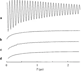
The signal induced by the inversion or saturation pulse can be removed by sub-tracting the signal obtained in an experiment without detection pulse (blind sig-nal). To get meaningful results, two different mw channels should be used for the preparation and the detection pulse. The blind signal is obtained with a fully attenuated detection pulse; all other parameters remain the same. With this pro-cedure not only the signal induced by the first pulse is subtracted but also spikes induced by other mw devices like the switches or the TWT amplifier are elimi-nated. The subtraction procedure is demonstrated in Fig. 2a and b for an SR experiment on natural dolomite. Figure 2a shows the original relaxation curve, while in Fig. 2b the blind signals are subtracted separately for each trace. The corrected relaxation curve is still slightly modulated. Although recording a blind signal doubles the measuring time, we used this approach in all the experiments.
a b C d 0 1 2 T(Its)
Fig. 2. SR-LOD T, experiment on Mn(II) centers in natural dolomite. a Initial relaxation curve af-ter reduction of each transient trace observed at a fixed T value to a single point. b With subtrac-tion of blind signals. c With a moving average over one modulasubtrac-tion period of the detecsubtrac-tion circuit.
2.2.2 Calculating the Moving Average over the Period TLCR
A modulation with frequency w and constant amplitude can be removed by cal-culating the moving average over a period Tp = 2 tIa or an integer multiple of
it. Since the relaxation curve observed in the IR-LOD T, and SR-LOD T,
ex-periments is often described by Eq. (1), superimposed by an exponentially damped cosine function with frequency 0LCR and time constant rLCR originating from the
preparation pulse, the moving average can be used to reduce the modulation. To show the efficiency of this approach, we discuss how the moving average influ-ences the relaxation time T„ what the residual is when the modulation is expo-nentially damped, and what the consequences are when TP is not exactly a
mul-tiple of the difference between two adjacent data points.
First we integrate M. in Eq. (1) over a time period 5 which is equivalent to a moving average over 8 with an infinite number of points in this interval
M^(t) = —f
[Meq
+ [Mz(0) – Meq ] exp — d t'
(3 ^-siz T
= Meq + smnh^ I [M(0) – Me, ] exp 7
J.
(2)The result shows that for 8 << Ti we get M(t) M.(t). If S is in the order of
T1, M(t) has still the same shape as M^, with the same relaxation time T, but
with amplitude T,l(S/2) Binh [(S/2)1T,] > 1. This has consequences if the decay
is multi-exponential. The relaxation curves with shorter T, values will become more intense relative to those with longer T, values.
For an exponentially damped cosine, s(t) = exp(–t/r)cos(wt) with time
con-stant r, integration over a modulation period Tp yields
t+R/()
s(t) = .T f exp
z
t)cos(wt')dt'z
^ (l +c^p/r) [wz z) r sin(wt) – cos(wt)] Binh ( -- . (3) In an LOD T, experiment with w = wLCR, t = T and r = TLCR = 2QLCR'wLCR with
QLCR >> 1, the ringing of the detection circuit after the preparation pulse, s(T) =
exp(–T/z-LCR)cos(WLCRT), is superimposed on the relaxation curve. The effect of the moving average can then be approximated by
s(T) ;; exp(—TIT ) sin(COLCR` )
2QLCR
(4)
This result shows that calculating a moving average over TLCR reduces the modu-lation by a factor 2QLCR (Fig. 2c). But for short T values, instrumental artifacts
T, Measurement with Longitudinal Detection 143
are still present. Therefore even when calculating a moving average over a modu-lation period, a blind signal should be subtracted. The result obtained after a moving average and subtraction of the blind signal is shown in Fig. 2d.
For an integration interval which deviates by 2AIco from Tp, we find
t+( r+/1 )!W (
_
f exp^—t)cos(wt')dt'
2(7t +
d) t-^n+a^^w
z
–
wz exp(–t1 r)
^exp i"
+
A ^[wa sin(wt– A) – cos(uot– A)]2(ii+A)(1+w z) wr
– exp^– ^^ A ^[wrsin(wt+ A) – cos(U)t+ A)] . (5)
With the assumptions A << 71 and QLCR >> 1, we obtain
s(T)
exp[–J[
cosA sin(WLCRT) – I sin cos (WLCRT) . (6)ZLCR 2QLCR ^ + A
There are two oscillatory terms in Eq. (6) which differ in phase by 900. The
sine function dominates if
A 1
< (7)
it 2QLCR
In this case, we find the same result as in Eq. (4), weighted by cosA. If the other term dominates, the amplitude of the unwanted modulation is
s(T)
exp(–T/TLCR)cos(WLCRT)(8)1+it/A
and the original modulation is reduced by a factor (1 + it/A). For example, for a moving average over 11 data points separated by 8 ns and an oscillation pe-riod of 84 ns, the error is 4 ns, corresponding to it/A = 21. The modulation am-plitude is reduced to about 4.5% of the initial value. If the remaining modula-tion is still too strong, the procedure can be repeated.
In all the calculations shown above, we assumed that the relaxation of M. is exponential. Otherwise the recovery curve would be distorted because only ex-ponential functions are not affected in their character by a moving average.
2.2.3 Two-Pulse Inversion Sequence
The LOD signal induced in the coil by the preparation sequence can also be minimized by an inversion sequence which consists of two pulses where the
l
oom
e it ^...,...,. ...
t(is)
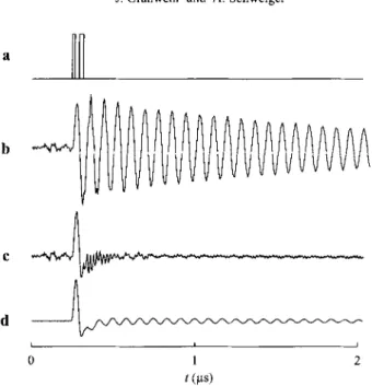
Fig. 3. Transient signal of DPPH observed during and after the two-pulse inversion sequence (with-out detection pulse). a Position and length of the pulses. b Only the first pulse was applied. c A second pulse is used to compensate the signal induced by the first pulse. d Inversion sequence with
subtraction of the blind signal with fully damped mw power.
second pulse annihilates the signal induced by the first pulse (Fig. 3a). A rule of thumb for the optimum choice of length, intensity and interpulse delay of the two pulses cannot be given, because this strongly depends on the relaxation times. The easiest way to adjust these parameters is to observe the transient signal on the oscilloscope and to optimize the different parameters iteratively.
In Fig. 3b, only the first pulse is applied, resulting in a signal with a large amplitude. When the second pulse is optimized for minimum modulation at the end of the preparation sequence, the signal shown in Fig. 3c is obtained. The modulation of the signal after subtraction of the blind signal is stronger than the signal without this correction (Fig. 3d). This is because some of the artifacts which were reduced by the second pulse are added again by subtracting the blind signal. However, the high-frequency artifacts are strongly reduced, and the in-strumental artifacts, which are clearly visible before the first pulse is applied, are completely removed.
2.3 Direct Measurement of Longitudinal Relaxation
An alternative way of measuring T, is to analyze the signal dMM(t)Idt which is
induced after the preparation sequence by the relaxing M magnetization. In anal-ogy to the IR-LOD T, and SR-LOD T, experiments, an exponentially damped modulation with frequency LCR and time constant TLCR originating from the
ring-T, Measurement with Longitudinal Detection 145
ing of the detection circuit is again superimposed on the relaxation curve. This time, only the instrumental artifacts can be removed by subtracting the blind signal which can be recorded either with a Bo field far off-resonance or by re-ducing the mw power. To reduce the oscillations superimposed on the dM^(t)/dt
relaxation curve, we have to calculate the moving average over TLCR as explained in the previous section. As a consequence, this method is only feasible for an exponentially relaxing magnetization.
With this direct method, T, can be determined in a single experiment so that the recording time is strongly reduced compared to an IR-LOD T, or SR-LOD T, experiment. Furthermore, it is possible to carry out a 2-D field-swept EPR experiment with T, as a second dimension. However, this method is only appro-priate for a small range of T, values. The lower limit is about 20 ns for the same reasons as discussed above for the IR-LOD T, and SR-LOD T, experiments. Since for this experiment the induced voltage is proportional to dMM(t)/dt, the
upper limit is in the order of 100 ns as the signal intensity scales with 1/T,. This becomes evident by calculating the first derivative of Eq. (1). In addition, instrumental problems such as long-range baseline drifts or features which can-not be removed by subtracting a blind signal are responsible for this small time interval.
An alternative to the calculation of the moving average is to perform the experiment with a resonant circuit with a very low QLCR value so that after excitation the ringing of the detection circuit decays rapidly (P. Hofer, pers. commun.).
3 Instrumentation
The instrumental setup has been described in detail in ref. 7. All the experiments presented here were performed on a Bruker X-band pulse EPR spectrometer with an ESP-380E pulse bridge and an ELEXSYS E580 pulse controller and signal processing unit. We used a Bruker X-band ENDOR probehead (EN 4118X), ro-tated about the sample axis by 90° so that the axis of the radio-frequency coil with inductance L 2.6 pH, acting as a pickup coil, was oriented parallel to the Bo field. One of the two semirigid cables from the coil to the ENDOR plugs at the outside of the probehead was short-circuited with the ground and acted as an inductance with a much smaller value than the inductance of the coil. The second semirigid cable was left open and operated as a capacitance to the ground with Cc - 50 pF. This already formed an LCR circuit with WLCR/27t 13 MHz and a quality factor at room temperature of QLCR > 100. The resonant frequency could be adjusted within a few megacycles by using a tunable air capacitor with CT = 5-15 pF in parallel to the capacitively coupled cable. The output voltage was detected with high impedance. The matching to the input impedance of the radio-frequency preamplifier (Avtech AV-141 C) was done actively with a volt-age follower (home-built). After preamplification, the signal was fed to the tran-sient recorder of the spectrometer (SpecJet), where the trantran-sient signals could be added with a high repetition rate.
This setup is much more sensitive than earlier designs because of the high filling factor of the detection coil, the high QLCR value, and the high resonant
frequency co,,, [7] which is kept constant throughout the whole experiment. 4 Results and Discussion
A sample of y-irradiated herasil glass (100 kGy) was measured with the IR-LOD T, pulse sequence at 298 K. To enhance signal intensity, the magnetization was two times refocused during the detection pulse of length 2.1 is by switching the mw phase by 180° after 420 and 1260 ns. The result is shown in Fig. 4 together with the residues between the observed and the fitted signal. A spin-lattice relaxation time of T, = 219 is was found. The same relaxation time was obtained with a standard IR experiment and two-pulse echo detection. The fit is slightly better by assuming a distribution of T, values (Fig. 4c) instead of a mono-exponential decay (Fig. 4b). This is reasonable because the strong y-irradiation leads to a high concentration of defect centers. Since this method of generating defects is not very specific, fluctuations of local defect concentrations may occur. In addition, in a glass the environment of the centers is not very well defined. As a second example, the SR-LOD T, method was used to study a natural dolomite at 250 K where two overlapping spectra with different longitudinal re-laxation behavior originating from Mn(II) that substitutes Ca(II) and Mg(II) can be observed (J. Granwehr et al., unpubl.). The relaxation curve shown in Fig. 5
a^ 1 0 200 400 600 800 0.05 T(is) b 0 -0.05 0.05 c 0 -0.05
Fig. 4. IR-LOD T, measurement of y-irradiated herasil glass at 298 K, B0 = 343.2 mT and v, =
9.614 GHz. The length of the inversion pulse was to = 22 ns, the length of the detection pulse was
2.1 µs with two phase changes. The nutation frequency was adjusted to c&cR• 400 data points were
collected. The acquisition time was 15 min, including the measurement of the blind signal. a Ex-perimental relaxation curve. b Residuals between the exEx-perimental relaxation curve shown in a, and the fitted curve assuming an exponential recovery of M_. c Residuals between the experimental
T, Measurement with Longitudinal Detection 147 a 0 0 1 2 0.005 T (ps) b 0 —0.005
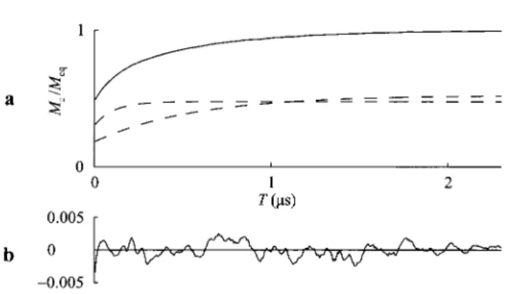
Fig. 5. SR-LOD T, measurement on Mn(II) centers in natural dolomite at 250 K, B0 = 352.2 mT
and mµ, = 9.622 GHz. The length of the saturation pulse was 420 ns, the length of the detection pulse was 44 ns. The mw power was 500 W for the saturation pulse and 150 W for the detection pulse. 400 data points were collected. The acquisition time was 15 min, including the measurement of the blind signal. a Solid line: experimental relaxation curve, smoothed with a moving average. Dashed lines: components of the relaxation curve obtained by the fitting of the experimental data.
b Residuals between the experimental curve and the sum of the fitted curves.
was obtained by calculating the moving average over TLcR. The longitudinal re-laxation times are found to be T,(1) = 110 ns and T,(2) = 568 ns.
As a last example, we determined the relaxation time T, of a powder of DPPH with the SR-LOD T, method, as well as the direct measurement of T,•
After recording the SR-LOD T, data consisting of 100 data points with a tran-sient recorder, three different procedures for data analysis have been used (Fig. 6). (a) In Fig. 6a, the amplitude of the spectral component at frequency wLCR of the signal for each T value after the detection pulse was determined, as in the previous examples. (b) A second approach for data analysis, shown in Fig. 6b, uses the sum of the two data points with maximum signal during the detection pulse. With the two approaches a and b for data analysis, time T between inver-sion and detection pulse was incremented step by step, leading to the SR-LOD T, relaxation curve. (c) In the third scheme, the same data set was used for a different analysis. Since Mz has fully relaxed for T> 400 ns (see Fig. 6a), the signal induced by the detection pulse does not depend on the preparation pulse anymore. Therefore for any of these traces the same result is expected in a di-rect measurement of T, when only the signal after the detection pulse is consid-ered. To increase the signal-to-noise ratio, the 50 traces with T> 500 ns were added before calculating two consecutive moving averages over TLcR. The result is shown in Fig. 6c. The relaxation times found with these three methods for data analysis are (a) T, = 59.2 ns, (b) T, = 56.7 ns, and (c) T, = 57.9 ns.
It should be noted that the first two methods which represent just two dif-ferent ways of analyzing the data provide basically the same information. The third method uses a different mechanism for measuring T, and can therefore be used to verify the results obtained with the first two schemes.
a 0.5 0 200 400 600 800 1000 T (ns) b 0.5 0 200 400 600 800 1000 T (ns) 0 c ou in —1 0 200 400 600 800 1000 t(ns)
Fig. 6. SR-LOD Ti measurement of a powder of DPPH at 298 K, B0 = 343.3 mT and mw = 9.630 GHz.
The length of the saturation pulse was 420 ns, the length of the detection pulse was 84 ns. The mw power was 500 W for both pulses. In the T dimension 100 points were recorded, separated by 10 ns. The acquisition time was 4 min, including the measurement of the blind signal. The solid lines repre-sent the experimental relaxation curves, the dashed lines are the corresponding fits. a From each trace in the t dimension the spectral component at rwruR was calculated. b Only the two data points with
maximum signal during the detection pulse were used. c Signal induced directly by the recovery of
M after the detection pulse, smoothed with two moving averages.
The same analysis of the relaxation curve after an mw excitation can be performed with the data from the example with the preparation sequence con-sisting of two pulses (Fig. 3d). In this case, it is sufficient to use a single mov-ing average over TLCR (curve not shown). A value of T, = 57.8 ns has been found in this experiment.
The relaxation times of DPPH have extensively been investigated in the lit-erature. Since Tz is between 10-8 and 10-' s and very close to the T, value, other recording techniques perform equally well. In ref. 10, for example, a value of T, = 56 ns was reported.
5 Conclusions
Longitudinal detection represents an alternative way to measure spin-lattice re-laxation times with IR and SR experiments. The approach overcomes most of the limitations inherent in conventional detection techniques. Echo formation is not required, and the method is free of the instrumental deadtime; high-power
T1 Measurement with Longitudinal Detection 149
mw pulses can be applied even during detection. As a consequence, a very broad range of T, values down to about 20 ns, independent of T2 or the ratio T1/T2, can be measured with the same method, and the data which represent the recov-ery of Mz are easy to analyze.
A blind signal recorded with a minimum of mw power for the detection pulse has to be subtracted to cancel the ringing of the detection circuit originating from the preparation pulse and to reduce instrumental artifacts. Another possibility to reduce the ringing is to split the inversion pulse into two pulses, where the nal induced in the detection circuit by the second pulse compensates for the sig-nal induced by the first pulse. However, in this case the various parameters have to be adjusted carefully, and an additional evolution time between the two pulses is introduced which may influence the result. With these techniques any relax-ation process can be investigated. If relaxrelax-ation is described as an exponential or a sum of exponentials, unwanted signals can be reduced by calculating a moving average over a period of the resonant frequency of the detection circuit.
The experiments which have been carried out on a commercial spectrometer with a commercial ENDOR probehead require a minimum of additional equip-ment, are easy to implement and can be performed routinely.
We described two schemes for data acquisition. In the first scheme the whole trace of the signal after the detection pulse is recorded. Each trace is then re-duced by an appropriate method to a single point in the relaxation curve. This approach has the advantage that by filtering, the desired information can be op-timized after data acquisition, and in some cases the data can be analyzed in different ways to verify the results. Another way of data acquisition is to inte-grate part of the signal with a boxcar. With this method it is not possible to selectively filter individual frequency components of the signal. But the blind sig-nal can directly be subtracted with a similar experimental procedure as is used for phase cycling, namely by altering the intensity of the detection pulse between two experiments instead of changing the phase. This is not possible on most spec-trometers when a transient signal is recorded.
We have also demonstrated that Ti can be determined by directly observing
the signal induced by the time-dependent magnetization during a relaxation pro-cess. In this case, the first derivative of the relaxation curve is recorded, in contrast to the IR and SR methods where the relaxation of M. is observed. The experiment is easy to perform, and one gets the whole relaxation curve in a single shot which reduces the measuring time considerably, even if several time traces have to be accumulated. Since the method is fundamentally different from the standard IR or SR experiments, it provides an additional means to verify the results, in particular because the information can be extracted from the same set of data. The applicability of the direct method is restricted to exponential relaxation processes with T, values between 20 and approximately 100 ns, which makes the technique an alternative only for a limited number of samples.
Acknowledgements
We thank Jorg Forrer for his technical support and Dr. Andreas Gehring for the dolomite sample. Furthermore we are grateful to Dr. Peter Hofer from Bruker Analytik GmbH for interesting discussions and for performing the experiment with the direct determination of T, with a similar setup. This work has been supported by the Swiss National Science Foundation.
References
I. Beck W.F., Innes J.B., Lynch J.B., Brudvig G.W.: J. Magn. Reson. 91, 12 (1991)
2. Hyde J.S. in: Time-Domain Electron Spin Resonance (Kevan L., Schwartz R.N., eds.), p. 1. New York: Wiley 1979.
3. Bloembergen N., Damon R.W.: Phys. Rev. 85, 699 (1952)
4. Strutz T., Witowski A.M., de Bekker R.E.M., Wyder P.: Appl. Phys. Lett. 57, 831 (1990) 5. Pescia J.: Ann. Phys. 10, 389 (1965)
6. Schweiger A., Ernst R.R.: J. Magn. Reson. 77, 512 (1988) 7. Granwehr J., Forrer J., Schweiger A.: J. Magn. Reson., in press.
8. Ernst R.R., Bodenhausen G., Wokaun A.: Principles of Nuclear Magnetic Resonance in One and Two Dimensions. Oxford: Clarendon Press 1987.
9. Hoffmann E., Schweiger A.: Appl. Magn. Reson. 9, 1 (1995)
10. Brandle R., Kruger G.J., Muller-Warmuth W.: Z. Naturforsch. 25, 1 (1970)
Authors' address: Arthur Schweiger, Physical Chemistry Laboratory, ETH Zentrum, CH-8092 Zurich,