HAL Id: hal-01796059
https://hal.archives-ouvertes.fr/hal-01796059
Submitted on 19 May 2018
HAL is a multi-disciplinary open access
archive for the deposit and dissemination of
sci-entific research documents, whether they are
pub-lished or not. The documents may come from
teaching and research institutions in France or
abroad, or from public or private research centers.
L’archive ouverte pluridisciplinaire HAL, est
destinée au dépôt et à la diffusion de documents
scientifiques de niveau recherche, publiés ou non,
émanant des établissements d’enseignement et de
recherche français ou étrangers, des laboratoires
publics ou privés.
Self-Organizing Maps, theory and applications
Marie Cottrell, Madalina Olteanu, Fabrice Rossi, Nathalie Villa-Vialaneix
To cite this version:
Marie Cottrell, Madalina Olteanu, Fabrice Rossi, Nathalie Villa-Vialaneix. Self-Organizing Maps,
theory and applications. Revista de Investigacion Operacional, 2018, 39 (1), pp.1-22. �hal-01796059�
Self-Organizing Maps, theory and applications
Marie Cottrell
1, Madalina Olteanu
1, Fabrice Rossi
1, Nathalie Villa-Vialaneix
21-SAMM - Université de Paris I
90 rue de Tolbiac
F-75013 Paris - France
marie.cottrell, madalina.olteanu, [email protected]
2-INRA, MIA-T, INRA, Université de Toulouse
F-31326 Castanet Tolosan - France
Abstract
The Self-Organizing Maps (SOM) is a very popular algorithm, introduced by Teuvo Kohonen in the early 80s. It acts as a non supervised clustering algorithm as well as a powerful visualization tool. It is widely used in many application domains, such as economy, industry, management, sociology, geography, text mining, etc. Many variants have been defined to adapt SOM to the processing of complex data, such as time series, categorical data, nominal data, dissimilarity or kernel data. However, so far, SOM has suffered from a lack of rigorous results on its convergence and stability. This article presents the state-of-art on the theoretical aspects of SOM, as well as several extensions to non numerical data and provides some typical examples of applications in different real-world fields.
RESUMEN
El algoritmo de auto-organización (Self-Organizing Map, SOM), o Mapa de Kohonen, es un algoritmo muy popular, definido por Teuvo Kohonen al principio de los anõs 80. El actúa como un algoritmo de clasificación (clustering) no supervisado y al mismo tiempo como una herramienta potente de visualización. El es ampli-amente usado para aplicaciones en muchos campos, tales como economía, industría, gestión, sociología, geografía, análisis de textos, etc. Muchas variantes han sido definidas para adaptar SOM al estudio de datos complejos, tales como series temporales, datos de categoría, datos nominales, datos de disimilaridades. Sin embargo, la convergencia y la estabilidad del algoritmo SOM no tienen pruebas rigurosas y completas hasta ahora. Este papel presenta el estado-del-arte de los aspectos teoréticos de SOM, al mismo tiempo que algu-nas extensiones para datos no numéricos y ejemplos típicos de diferentes campos con datos reales.
Keywords SOM, Batch SOM, Stability of SOM, KORRESP, Relational and kernel SOM
1. Introduction
This review is widely inspired by an invited paper [18] presented during the WSOM 2016 Conference, at Houston (USA) in January 2016, which addressed the Theoretical and Applied Aspects of the Self-Organizing Maps.
The self-organizing map (SOM) algorithm, defined by T. Kohonen in his first articles [40], [39] is a very famous non-supervised learning algorithm, used by many researchers in different application domains (see e.g. [37, 53] for surveys). It is used as a powerful clustering algorithm, which, in addition, considers a neighborhood structure among the clusters. In this way, close data belong to the same cluster (as in any other clustering algorithm) or to neighboring clusters. This property provides a good visualization of multidimensional data, since the clusters can be displayed according to their neighborhood structure. Furthermore, the SOM algorithm is easy to implement and as its complexity is linear with respect to the number of data, it is well-adapted to Big Data problems.
Its basic version is an on-line stochastic process, inspired by biological paradigms as it was explained in the first Kohonen’s articles. It models the plasticity of the synaptic connections in the brain, where the neural connections either strengthen or disappear during “learning” phases, under the control of the practical experience and received inputs, without supervision.
For industrial applications, it can be more convenient to use a deterministic version of SOM, in order to get the same results at each run of the algorithm when the initial conditions and the data remain unchanged. To address this issue, T. Kohonen has introduced the batch SOM in [42, 44].
Figure 1: Neighborhood functions
Over time, the researchers have defined many variants of SOM, some of them will be presented below. First the modified versions of SOM meant to achieve the goal of overcoming some theoretical difficulties of the original algorithm. But nowadays, SOM variants are being designed to deal with non numerical data (categorical data, abstract data, similarity or dissimilarity indices, for example).
The paper is structured as follows: Section 2 focuses on the definition of the original SOM algorithm designed for numerical data and on the main mathematical tools that are useful for its theoretical study. Section 3 is devoted to the simplest case, the one-dimensional setting, for which the theoretical results are the most complete. The multidimensional case is addressed in Section 4 together with some real-world examples. Sections 5 and 6 are dedicated to the definition of Batch SOM and of other interesting variants. In Section 7, we show how it is possible to extend the original SOM to non numerical data, and we distinguish between the extensions to categorical data and to dissimilarity or kernel data. The conclusion in section 8 provides some directions to go further.
2. SOM for numerical data
Originally in [40] and [39], the SOM algorithm was defined for data described by numerical vectors which belong to a subsetX of an Euclidean space (typicallyRp). For some results, we need to assume that the subset is bounded and convex. Two different settings have to be considered from the theoretical point of view:
• the continuous setting: the input spaceX in Rpis modeled by a probability distribution with a density function f ,
• the discrete setting: the input spaceX comprises N data points x1, . . . , xNinRp. Here the discrete setting means a finite
subset of the input space.
The data can be stored or made available on-line.
2..1. Neighborhood structure
Let us take K units on a regular lattice (string-like for one dimension, or grid-like for two dimensions).
IfK = {1,...,K } and t is the time, a neighborhood function h(t) is defined on K ×K . If it is not time-dependent, it will be denoted by h. It has to satisfy the following properties:
• h is symmetric and hkk= 1,
• hkldepends only on the distance dist(k, l ) between units k and l on the lattice and decreases with increasing distance.
Several choices are possible, the most classical is the step function equal to 1 if the distance between k and l is less than a specific radius (this radius can decrease with time), and 0 otherwise.
Another very classical choice is a Gaussian-shaped function
hkl(t ) = exp à −dist 2(k, l ) 2σ2(t ) ! ,
whereσ2(t ) can decrease over time to reduce the intensity and the scope of the neighborhood relations. For example, Figure 1 shows some classical neighborhood functions.
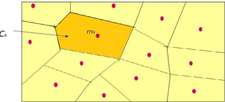
Figure 2: ct(x) = k ⇐⇒ mk(t ) is the winning prototype of x
2..2. On-line SOM
A prototype mk∈ Rp is attached to each unit k, the initial values of the prototypes are chosen at random and denoted by
m(0) = (m1(0), . . . , mK(0)). The SOM algorithm (in its on-line stochastic version) is defined as follows:
• At time t , a data point x is randomly drawn (according to the density function f (continuous setting) or in the finite set X (discrete setting),
• The Best Matching Unit is defined by
ct(x) = arg min
k∈{1,...,K }kx − mk(t )k
2
, (1)
• All the prototypes are updated via
mk(t + 1) = mk(t ) + ε(t)hkct(x)(t )(x − mk(t )), (2)
whereε(t) is a learning rate (positive, <1, constant or decreasing).
After learning, cluster Ckis defined as the set of inputs closer to mkthan to any other one. The result is a data space
partition (Figure 2), called Voronoï tesselation, with a neighborhood structure between the clusters. The Kohonen map is the representation of the prototypes or of the cluster contents displayed according to the neighborhood structure.
The properties of the Kohonen maps are of two kinds:
• the quantization property, i.e. the prototypes represent the data space as accurately as possible, as do other quantization algorithms;
• the self-organization property, that means that the prototypes preserve the topology of the data: close inputs belong to the same cluster (as do any clustering algorithms) or to neighboring clusters.
To get a better quantization, the learning rateε decreases with time as well as the scope of the neighborhood function h.
2..3. Theoretical concerns
The algorithm is, therefore, very easy to define and to use, and a lot of practical studies confirm that it works. But, in fact, the theoretical study of its convergence when t tends to +∞ remains without complete proof and provides open problems ([8] and [25]). Note that this problem departs from the usual convergence problem addressed in Machine Learning Theory, where the question is to know if the solution obtained from a finite sample converges to the true solution that might be obtained from the true data distribution.
When t tends to +∞, the Rp-valued stochastic processes (mk(t ))k=1,...,K can present oscillations, explosion to infinity, convergence in distribution to an equilibrium process, convergence in distribution or almost sure to a finite set of points inRp, etc.
Some of the open questions are:
• Is the algorithm convergent in distribution or almost surely, when t tends to +∞? • What happens whenε is constant? when it decreases?
• If a limit state exists, is it stable? • How to characterize the organization?
2..4. Mathematical tools
The convergence problem of SOM can be addressed with tools usually used to study the stochastic processes. One can empha-size on three main theories.
• The Markov Chain theory for constantε and h, to study the convergence and the limit states.
– If the algorithm converges in distribution, this limit is an invariant measure for the Markov Chain; – If there is strong organization, it has to be associated to an absorbing class.
• The Ordinary Differential Equation method (ODE) If for each k ∈ K , Equation (2) is written in a vector form:
m(t + 1) = m(t) − ε(t)Φ(x,m(t)), (3) whereΦ is a stochastic term, then the ODE (Ordinary Differential Equation) which describes the mean behavior of the process is
d m
d t = −φ(m), (4)
whereφ(m) is the expectation of Φ(.,m). Then the kt h−component of φ is
φk(m) = K X j =1 hk j Z Cj (x − mk) f (x)d x (5)
for the continuous setting or
φk(m) = 1 N K X j =1 hk j X xi∈Cj (xi− mk) = 1 N N X i =1 hkc(xi)(xi− mk) (6)
for the discrete setting.
Therefore the possible limit states are solutions of the equation
φ(m) = 0.
If the zeros of functionφ are minimum values of a function (called Energy Function), one can apply the gradient descent methods to compute the solutions.
• The Robbins-Monro algorithm theory is used when the learning rate decreases under the conditions X
t ε(t) = +∞ and Xt ε(t)
2
< +∞. (7)
Despite the power of these mathematical tools, the original SOM algorithm is difficult to study for several reasons: • for p > 1, it is not possible to define any absorbing class which could be an organized state;
• although m(t ) can be written down as a classical stochastic process, Erwinn et al., 1992, [22, 23], have shown that it does not correspond to any energy function, or in another words that the SOM algorithm is not a gradient descent algorithm in the continuous setting;
• finally, no demonstration takes into account the variation of the neighborhood function. All the existing results are valid for a fixed scope and intensity of the function h.
3. The one-dimensional case
This case is very simplified and far from the applications: the dimension p = 1, the data space X = [0,1], the neighborhood structure is a string lattice, the data is distributed according to a uniform density and the parameterε is constant. But it is the first case totally rigorously studied by Cottrell and Fort in 1987 [7].
They prove the following results:
Theorem 1. Simplest case
Ifε is a constant <1/2 and if the neighborhood of k is {k − 1,k,k + 1}, • The number of badly ordered triplets is a decreasing functional;
• The hitting time of the absorbing class is almost surely finite;
• The process m(t ) converges in distribution to a monotonous stationary distribution which depends onε.
Figure 3. illustrates the first part of the theorem. The neighbors of j are j − 1 and j + 1. The values of the prototypes are on the y-axis, in [0, 1]. On the left, the first two triplets are not ordered. SOM will order them with a strictly positive probability. At right, the last two triplets are well ordered and SOM will never disorder them.
0 1
j − 1 j j + 1 j − 1 j j + 1 j − 1 j j + 1 j − 1 j j + 1
Figure 3: Four examples of triplets of prototypes, (mj −1, mj, mj +1)
Another result is available in the same frame, but whenε is decreasing, see [7].
Theorem 2. Decreasingε
Ifε(t) −→ 0 and satisfies the Robbins-Monro conditions
X
t ε(t) = +∞ and Xt ε(t)
2
< +∞, (8)
after ordering, the process m(t ) a.s. converges towards a constant monotonous solution of an explicit linear system.
Some results about organization and convergence have been obtained a little later by Bouton, Fort and Pagès, [6, 27], in a more general case.
Theorem 3. Organization
One assumes that the setting is continuous and that the neighborhood function is strictly decreasing from a certain distance between the units.
• The set of ordered sequences (increasing or decreasing sequences, i.e. organized ones) is an absorbing class; • Ifε is constant, the hitting time of the absorbing class is almost surely finite.
Theorem 4. Convergence
One assumes that the setting is continuous, the density is log-concave, the neighborhood function is time-independent and strictly decreasing from a certain distance between units.
• If the initial state is ordered, there exists a unique stable equilibrium point (denoted by x∗);
• Ifε is constant and the initial disposition is ordered, there exists an invariant distribution which depends on ε and which concentrates on the Dirac measure on x∗whenε −→ 0;
• Ifε(t) satisfies the Robbins-Monro conditions (8) and if the initial state is ordered, then m(t) is almost surely convergent towards this unique equilibrium point x∗.
It is clear that even in the one-dimensional case, the results are not totally satisfactory. Although the hypotheses on the density are not very restrictive, some important distributions, such as theχ2or the power distribution, do not fulfill them. Furthermore, nothing is proved, neither ifε(t) is a decreasing function to ensure ordering and convergence simultaneously,
nor for a neighborhood function with a decreasing scope, whereas in practical implementations it is always the case.
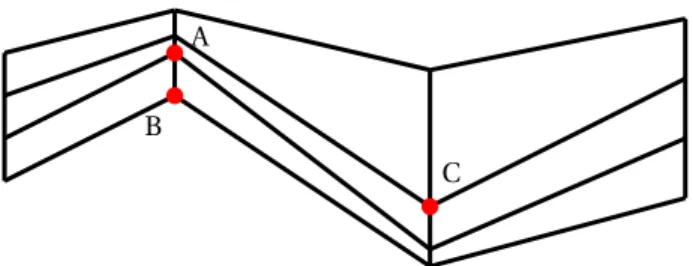
4. The Multidimensional Case
In the multidimensional case, most of the previous results do not hold. For example, no absorbing class has been found when the dimension is greater than 1. Figure 4. is an illustration of such case, in dimension 2 with 8 neighbors: even if the x- and y-coordinates are ordered, it is possible (with positive probability) to disorder the prototypes.
B A
C
Figure 4: Disordering an ordered configuration. A is a neighbor of C, but B is not a neighbor of C. If C is very often the best matching unit, B is never updated, whereas A becomes closer and closer to C. Finally, the y− coordinate of A becomes smaller than that of B and the disposition is disordered.
4..1. Continuous setting
Let p be the data dimension. Assume that h andε are constant. Sadeghi (2001) [60] proves the following result:
Theorem 5. If the probability density function f is positive on an interval, the algorithm weakly converges to a unique probability
distribution which depends onε.
Assuming p = 2 and denoting by F++the set of the prototypes with simultaneously increasing coordinates, these two apparently contradictory results hold.
Theorem 6. For a constantε and very general hypotheses on the density f ,
• the hitting time of F++is finite with a positive probability (Flanagan, 1996, [24]);
• but in the 8-neighbor setting, the exit time is also finite with positive probability (Fort & Pages, 1995, [26]).
However, in practical applications, the algorithm converges towards a stable equilibrium!
4..2. Discrete setting
For the continuous setting, we know that SOM is not a gradient descent algorithm (Erwinn, 1992, [22, 23]). But the discrete setting is quite different, since the stochastic process m(t ) derives from an energy function (if h is not time-dependent). This is a very important result, since in applications such as data mining or clustering, the data is always discrete.
For the discrete setting, Ritter et al., 1992, [57], prove the next theorem:
Theorem 7. In the discrete setting, SOM is a gradient descent process associated to
E (m) = 1 2N N X i =1 K X k=1 hkc(xi)kmk− xik2, (9)
called Extended Distortion or Energy Function.
Note that this energy function can also be written in a more explicit manner as
E (m) = 1 2N K X k=1 K X j =1 hk j X xi∈Cj kmk− xik2. (10)
This result does not ensure the convergence, since the gradient of the energy function is not continuous on the boundaries of the clusters. But this energy has an intuitive meaning, because it combines two criteria : a clustering criterion and a correct organization criterion.
Note that in the 0-neighbor setting, SOM reduces to the Vector Quantization process (VQ), the energy reduces to the clas-sical distortion (or within-classes sum of squares)
E (m) = 1 2N N X i =1 kmc(xi)− xik 2.
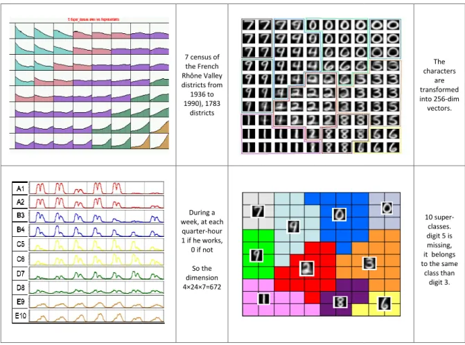
7 census of the French Rhône Valley districts from 1936 to 1990), 1783 districts During a week, at each quarter-hour 1 if he works, 0 if not So the dimension 4×24×7=672 The characters are transformed into 256-dim vectors. 10 super-classes. digit 5 is missing, it belongs to the same class than digit 3.
Figure 5: Ex. 1: clustering of districts (top left), Ex.2: workers schedules (bottom left), Ex. 3: manuscript characters (the super-classes at top right and the contents on bottom right.
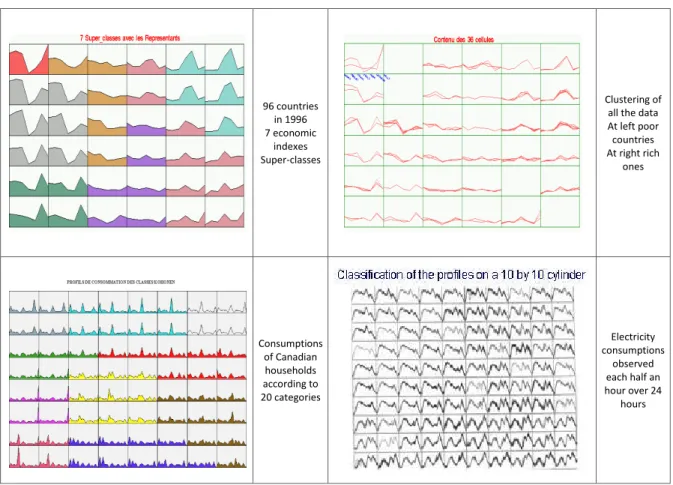
96 countries in 1996 7 economic indexes Super-classes Clustering of all the data At left poor countries At right rich ones Consumptions of Canadian households according to 20 categories Electricity consumptions observed each half an hour over 24 hours
Figure 6: Ex. 4: countries (the prototypes on top left and the contents on top right), Ex. 5: domestic consumption (the prototypes on bottom left), Ex. 6: power consumption (the contents on bottom right).
4..3. Examples of practical applications
Figures 5 and 6 present some examples of Kohonen maps. The prototypes are displayed on the lattice and clustered into super-classes easier to describe, by using a Hierarchical Classification. The organization is confirmed since the super-super-classes group only neighboring prototypes.
In Ex. 1 (Figure 5) [9], there are 1783 districts in the French Rhône Valley, the dimension is 7, the variables are 7 census collected in 1936, 1954, 1962, 1968, 1975, 1982, 1990. The Kohonen map is a 8 × 8 grid. The data are grouped into 5 super-classes using a Hierarchical Clustering of the 8 × 8 prototypes. For Ex. 2 [49], in a week, at each quarter-hour, a binary code is filled by each worker: 1 if he works, 0 otherwise. Each observation is a 4 × 24 × 7 = 672-dimensional vector and there are 566 workers. The Kohonen map is a 10-units string, and the figure shows the 10 prototypes, grouped into 5 super-classes. In Ex. 3 [15], one sees the 10 colored super-classes, and below all the manuscript digits coded as 256-dimensional vectors are drawn in the Kohonen classes.
In Ex. 4 (Figure 6) [3] [12], 96 countries are described by 7 ratios (annual population growth, mortality rate, illiteracy rate, population proportion in high school, GDP per head, unemployment rate, inflation rate) in 1996. The prototypes are displayed on a 6 × 6 Kohonen map and grouped into 7 super-classes. Ex. 5 [9] concerns the distribution of Canadian consumers based on 20 consumption categories. And Ex. 6 [10] displays the contents of each Kohonen class, on a 10 × 10 cylindrical map, after learning, where each observation is the daily electrical consumption in France measured each half an hour over 24 hours over 5 years.
Figure 7: Batch SOM
5. Deterministic Batch SOM
In some practical applications, it is preferable to use a deterministic version of SOM, in order to get reproducible results when the initial prototype values are fixed, [42, 44].
The idea is to compute the solutions directly, without any on-line learning and to use all the data at each iteration. It is known that the possible limit states of the SOM algorithm are solutions of the ODE equationφ(m) = 0, so it is natural to solve it.
For the continuous setting, one gets
m∗k= PK j =1hk j R Cjx f (x)d x PK j =1hk j R Cjf (x)d x . and in the discrete setting, the analogous is
m∗k= PK j =1hk jPxi∈Cjxi PK j =1hk j|Cj| = PN i =1hkc(xi)xi PN i =1hkc(xi) .
Therefore, the limit prototypes m∗kare the weighted means of all the inputs which belong to the cluster Ckor to its
neigh-boring clusters. The weights are given by the neighborhood function h.
From this remark, Kohonen [42, 44], derives the definition of the Batch SOM, which directly computes the limit prototypes
m∗ k, by mk(t + 1) = PK j =1hk j(t ) R Cj (mk (t))x f (x)d x PK j =1hk j(t ) R Cj (mk (t))f (x)d x (11) for the continuous setting, and
mk(t + 1) = PN i =1hkct(x i)(t )xi PN i =1hkct(x i)(t ) (12) for the discrete case.
The initial values of the prototypes are chosen at random as usual. Figure 7 shows the limit prototypes as mean values of the union of its cluster and of the neighboring clusters.
For Batch SOM, the theory is a little more achieved, since it is proven by Fort et al., [28, 29], that it is a quasi-Newtonian algorithm associated to the Extended Distortion and that it converges to one of its local minima. Note that in the 0-neighbor setting, Batch SOM reduces to Forgy process (k-means, or what is also called Moving Centers), which converges towards a local minimum of the Distortion. Table 1 summarizes the relations between four clustering algorithms: the on-line SOM, the Batch SOM, the Vector Quantization (VQ) and the Forgy algorithm (or Moving Centers).
Some remarks highlight these relations:
• VQ and Forgy algorithms are 0-neighbor versions of on-line and Batch SOMs respectively;
• SOM and Batch SOM preserve the data topology: close data belong to the same cluster or to neighboring clusters; • The Kohonen maps have good visualization properties whereas the 0-neighbor algorithms (Forgy and VQ) do not;
Stochastic Deterministic 0 neighbor VQ, SCL Forgy, Moving Centers
With neighbors SOM Batch SOM
Table 1: Comparison summary
• SOM depends very little on the initialization, whereas Batch SOM is very sensitive to it; • Batch SOM is deterministic and often preferred for industrial applications.
6. Variants of SOM
Several variants have been defined to improve the SOM properties or to recast the SOM algorithm into a probabilistic frame-work.
6..1. Hard assignment in the Heskes’rule
One of the most important variants has been introduced by Heskes, 1999 [34], who has proposed a modification of the best-matching unit assignment, in order to get continuous gradient of the energy function.
Equation (1) is re-written ct(x) = arg min k∈{1,...,K } K X j =1 hk j(t )kx − mk(t )k2. (13)
With the Heskes rule, the energy function is continuous for both discrete and continuous settings, and its gradient is also continuous in the continuous setting. So this modified SOM is a gradient descent process of the Energy Function
E (m) =1 2 K X j =1 K X k=1 hk j(t ) Z x∈Cj(m) kx − mk(t )k2f (x)d x. (14)
in the continuous setting.
6..2. Soft Topographic Mapping - STM
The original SOM algorithm is based on a hard winner assignment. Generalizations based on soft assignments were derived in [31] and [34].
First we remark that the energy function in the discrete SOM can be written as:
E (m, c) =1 2 K X k=1 N X i =1 ci k K X j =1 hk j(t )kmj(t ) − xik2,
where ci kis equal to 1 iif xibelongs to cluster k.
Then the crisp assignment is smoothed by considering ci k≥ 0 such thatPKk=1ci k= 1, so that ci k= P(xi∈ Ck).
Finally, a deterministic annealing scheme is used to avoid local minima: the energy function is transformed into a “free energy” cost function,
F (m, c,β) = E(m,c) −1 βS(c) ,
whereβ is the annealing parameter.
It can be proven that for fixedβ and h, the minimization of the free energy leads to iterating over two steps P(xi∈ Ck) = exp(−βei k) PK j =1exp(−βei j) , (15) where ei k=12 PK j =1hj k(t )kxi− mj(t )k2and
mk(t + 1) = PN i =1xiPKj =1hj k(t )P(xi∈ Cj) PN i =1 PK j =1hj k(t )P(xi∈ Cj) . (16)
Ifβ ≈ 0, there is only one global minimum computed by a gradient descent or EM schemes. When β → +∞, the free energy
tends to be E (m, c), the classical batch SOM is retrieved and most of the local minima are avoided. The deterministic annealing minimizes the free energy, starting from a smallβ, to finally get (with increasing β) an approximation of the global minimum
of E (m, c).
6..3. Probabilistic models
Other variants of SOM use a probabilistic framework. The central idea of those approaches is to constrain a mixture of Gaussian distributions in a way that mimics the SOM grid.
Consider a mixture of K Gaussian distributions, centered on the prototypes, with equal covariance matrix, • In the Regularized EM [35], the constraint is enforced by a regularization term on the data space distribution;
• In the Variational EM, [61], the constraint is induced at the latent variable level (via approximating the posterior bution of the hidden variables knowing the data points p(Z |X ,Θ), where Θ is the parameter vector, by a smooth distri-bution);
• In the Generative Topographic Mapping, the constraint is induced on the data space distribution, because the centers of the Gaussian distributions are obtained by mapping a fixed grid to the data space via a nonlinear smooth mapping. One can find more details about these SOM variants in the WSOM 2016 Proceedings [18]. All the probabilistic variants enable missing data analysis and easy extensions to non numerical data.
7. SOM for non numerical data
The original definition of SOM was conceived to deal with vector numerical variables. Quickly, Teuvo Kohonen and other researchers[41], [43], [36], [38], [45], [48], [46], [47], [17] have proposed adaptations of SOM to categorical variables as those collected in surveys and for text mining.
SOM algorithm may be adapted to :
• Categorical data, like survey data, where the variables are answers to questions with multiple choices, or counting tables, where items are classified according to multiple criteria;
• Data described by a dissimilarity matrix or a kernel, where the observations are known by their pairwise relations. This framework is well adapted to data like graphs, categorical time series, etc.
7..1. Contingency data
The adaptation of the SOM algorithm to contingency data (named KORRESP) was first defined by Cottrell et al. in 1993 [16]. The data consists in a contingency table which crosses two categorical variables and which is denoted by T = (ti , j) with I rows and J columns. The idea is to mimic the Factorial Correspondence Analysis, which consists in two simultaneous weighted Principal
Component Analysis of the table and of its transposed, using theχ2distance instead of the Euclidean distance.
Therefore, to be able to take into account theχ2distance and the weighting, to comply with the way it is defined in the Multiple Correspondence Analysis. After transforming the data, two coupled SOMs using the rows and the columns of the transformed table can thus be trained. In the final map, related categories belong to the same cluster or to neighboring clusters. The reader interested in a detailed explanation of the algorithm can refer to [4]. More details and real-world examples can also be found in [11, 13]. Note that the transformed tables are numerical data tables, so there is no particular theoretical results to comment on. All the results that we presented for numerical data still hold.
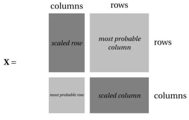
So the algorithm KORRESP can be defined in three steps:
• First, scale the rows and the columns as in Factorial Correspondence Analysis and replace the table T by the scaled contingency table denoted by Tsc, where
ti , jsc = ti , j pti .t. j
with ti .=Pjti jand t. j=Piti j;
• Then build an extended data table X by associating to each row, the most probable column and to each column, the most probable row;
• Finally, simultaneously classify the rows and the columns onto a Kohonen map, by using the extended data table X as input for the SOM algorithm.
The approach is summarized in the scheme Figure 8.
X =
columns rows
columns rows
most probable row
most probable column
scaled column scaled row
Figure 8: The extended data table X
Note that the assignment step uses the scaled rows or columns, the prototype update concerns the extended rows or columns and that the same are alternatively drawn at random. After convergence, rows and columns items are simultaneously classified as in FCA, but on one map only.
In real world applications, the data can be collected in surveys or text mining and can be more complex than a simple contingency table crossing two questions. They can be collected as a Burt Table, i.e. a full contingency table for more than two questions or a complete disjunctive table that contains the answers of all the surveyed individuals. KORRESP deals with all these kinds of tables. It is sufficient to consider these tables as“contingency tables” crossing their rows and their columns.
Let us take a simple example to illustrate the KORRESP algorithm. Table 2 displays the distribution of the 12,585 mon-uments listed in France in 1990, according to their category (11 levels) and their owners (6 levels) [16]. We use a KORRESP algorithm to simultaneously cluster the categories of monuments and their owners on a 5 × 5 Kohonen map.
Table 3 presents the resulting Kohonen map after learning, which shows the main associations between monument cate-gories, between owners types, between monument categories and owner types. One can see, for example, that the cathedrals (CAT) and the state (ST_) are in the same cluster, as foreseen since the cathedrals in France belong to the State. Similarly, the castles (CAS), the private secular monuments (PRI) are with the Owner Private (PR_). The churches and the chapels belong to the towns in France and, as expected, are close to the owner Town (TO_).
The Kohonen map gives interesting information on these associations, in line with the results obtained by using a Factorial Correspondence Analysis, on one map only, while many projections are required to correctly interpret the results of a Factorial Analysis.
7..2. Median SOM
When the data are known only through relational measures of ressemblance or dissemblance, such as kernels or dissimilarity matrices, it is also possible to extend the original SOM algorithm. Both on-line and batch versions were proposed during the last two decades. These versions can be used for data-like graphs (social networks) or sequences (DNA sequences) for example. A detailed review of these algorithms is available in [58].
The data is supposed to be described by a symmetric (dis)similarity matrix D = (δ(xi, xj))i , j =1,...,N, in a discrete setting.
Note that observations (xi) do not necessarily belong to a vector space.
One of the first attempts was proposed by Kohonen and Somervuo, 1998, [38], and is the Median SOM. The prototypes have to be equal to an observation. The optimal prototypes are computed by searching through (xi)i =1,...,N, instead ofX , as in [38],
[48], [20], [21].
The Median SOM algorithm is defined by a discrete optimization scheme, in a batch mode: 1. Assignment of all data to their best matching units: ct(xi) = argminkδ(xi, mk(t ));
2. Update of all the prototypes within the dataset by mk(t ) = argminxi
PN
j =1hct(x
j)k(t )δ(xi, xj).
As the algorithm explores a finite set, it is convergent to a local minimum of the energy function. But there are some drawbacks: all prototypes must belong to the data set, and the induced computational cost is very high.
Monument Town Private State Department Public Establishment) Other
(TO_) (PR_) (ST_) (DE_) (PU_) (OT_)
Prehistoric antiquities (PRE) 244 790 115 9 12 144
Historical antiquities (HIS) 246 166 46 23 11 31
Castles and manors (CAS) 289 964 82 58 40 2
Military architecture (MIL) 351 76 59 7 2 0
Cathedrals (CAT) 0 0 87 0 0 0
Churches (CHU) 4298 74 16 5 4 2
Chapels and oratories (CHA) 481 119 13 7 8 4
Monasteries (MON) 243 233 44 37 18 0
Public secular monuments (PUB) 339 47 92 19 41 2
Private secular monuments (PRI) 224 909 46 7 18 4
Others (OTM) 967 242 109 40 10 9
Table 2: Historical monuments classified by category and kind of owners, 1990, France, Source MCC/DPVDEP
7..3. Relational SOM
Another class of algorithms well adapted to data known by a dissimilarity matrix relies upon a result obtained by Goldfarb, 1984 [30], which shows that if the data is described by a (dis)similarity matrix D = (δ(xi, xj))i , j =1,...,n, they can be embedded in a
pseudo-Euclidean space:
Theorem 8. There exist two Euclidean spacesE1andE2andψ1: {xi} → E1,ψ2: {xi} → E2such that
δ(xi, xj) = kψ1(xi) − ψ1(xj)kE21− kψ2(xi) − ψ2(xj)k2E2.
The principle of the adapted algorithm is to use the data representation inE = E1⊗ E2, whereψ(x) = (ψ1(x),ψ2(x)).
• The prototypes are expressed as convex combinations of the (ψ(xi)): mk(t ) = N X i =1 γt kiψ(xi) whereγt ki≥ 0 and P iγtki= 1;
• The distance kψ(xi) − mk(t )k2Ecan be expressed with D and theγ by
³ Dγtk ´ i− 1 2(γ t k) T Dγtk. where ³ γt k ´T = ³ γt k,1, ...,γ t k,N ´ .
Then the first step of the algorithm, finding the best matching unit of an observation, as introduced in Equation (1), can be directly generalized to dissimilarities, both for on-line and batch settings. As for the prototype update, it should be noted that it only concerns the coordinates (γk).
PRE HIS MIL CHU OT_ OTM CHA TO_ CAS PRI PR_
MON PUB CAT
DE_ ST_
PU_
Table 3: The monuments, their categories and their owners on the Kohonen map
γt +1 k = γ t k+ ε(t )hkct(x i)(t ) ³ 1i− γtk ´ (17) where xiis the current observation and 1i l= 1 iif l = i and 0 otherwise.
In the batch framework [33], [32], the prototypes update is identical to the original Batch algorithm (see Equation (12)). One puts mk(t + 1) = N X i =1 hkct(x i)(t ) PN j =1hkct(x j)(t ) ψ(xi) ⇔ γt +1ki = hkct(x i)(t ) PN j =1hkct(x j)(t ) . (18)
If the dissimilarities are in fact given by Euclidean distances between data points inRp, the relational SOM is strictly equiv-alent to the original SOM.
7..4. Kernel SOM
A kernel K = (K (xi, xj))i , j =1,...,Nis a particular case of symmetric similarity measure, positive semi-defined and satisfying
∀ M > 0, ∀ (xi)i =1,...,M∈ X , ∀ (αi)i =1,...,M,
X
i , j
αiαjK (xi, xj) ≥ 0.
Observe that a kernel matrix K is a Euclidean dot product, but that a dissimilarity matrix D may not necessarily be trans-formed into a kernel matrix. For kernel data, Aronszajn, 1950, [1] proves the following result:
Theorem 9. There exists a Hilbert spaceH , also called feature space, and a mapping ψ : X → H , called feature map, such that
K (xi, xj) = 〈ψ(xi),ψ(xj)〉H(dot product inH ).
The SOM algorithm can be extended to kernel SOM (see [62], [50]), following the steps mentioned below: • The prototypes are expressed as convex combinations of the (ψ(xi)) :
mk(t ) = N X i =1 γt kiψ(xi) whereγt ki≥ 0 and P iγtki= 1;
• The distance is given by
kψ(xi) − mk(t )k2= ³ γt k ´T Kγt k− 2Kiγ t k+ Ki i,
where Kiis the i th row of K and
³ γt k ´T = ³ γt k,1, ...,γ t k,N ´ .
The prototype updates are the same as before, acting only on theγ. Note that if the dissimilarity is the squared distance induced in the feature spaceH , kernel SOM and relational SOM are strictly equivalent.
The algorithms are fully equivalent to the original SOM algorithms for numerical data in the feature (implicit) Euclidean space induced by the dissimilarity or the kernel, as long as the prototypes are initialized in the convex hull of the input data. So the relational/kernel versions suffer from the same theoretical limitations as the original SOM algorithms.
Figure 9: Graph of co-occurrences for the characters in Les Misérables
7..5. Example: The characters in "Les misérables"
This example is extracted from the paper by Olteanu and Villa, 2015, [55]. Let us define the graph of co-occurrences (in the same chapter) of the 77 characters in the Victor Hugo’s novel “Les misérables”. It is displayed in Figure 9.
The dissimilarity between two characters is defined as the length of the shortest path between two vertices. The resulting Kohonen map using the relational on-line version is displayed in Figure 10 at left. A hierarchical clustering of the prototypes is used to build “super-classes”, which are displayed in Figure 10 at right, where the size of the clusters is proportional to the number of characters.
In Figure 11 at left, one can color the characters in the initial graph with the color of the super-classes. Figure 11 at right presents a simplified graph, built from the super-classes. Each super-class is represented by a circle with a radius proportional to the number of vertices it contains. The width of the edges is proportional to the number of connections between two super-classes.
7..6. Example: Professional trajectories
The data comes from a project “Generation 98 à 7 ans”, 2005, of CEREQ, Centre Maurice Halbwachs (CMH), France. To collect the data, 16,040 young people leaving initial training in 1998 are observed over 94 months. Each month, the nature of their ac-tivity is recorded (permanent labor contracts, fixed-term contracts, apprenticeship program, public temporary-labor contract, on-call contract, unemployment, inactive, military service, education,...).
The dissimilarity between recorded sequences is defined as the Optimal Matching, which is a variant of the Edit Distance where some costs are assigned to the changes. After the relational SOM is trained on the entire data set, one gets the final map illustrated in Figure 12 [54].
8. Conclusion and Perspectives
We have presented the original on-line and Batch SOM, as well as some of their variants. Although many practical evidences do not have rigorous mathematical proofs so far, these algorithms are widely used to solve a large range of problems. The extensions to categorical data, dissimilarity data, kernel data have transformed them into even more powerful tools. Since the Heskes’s variants of SOM have a more solid theoretical background, SOM can appear as an easy-to-develop approximation of these well-founded algorithms. This observation should ease the concern that one might experience about it.
Figure 10: The Kohonen map and the super-classes of characters
Figure 12: Top left: exclusion of the labor market. Top right: quick integration
Their non supervised learning characteristic makes them very interesting to use for exploratory data analysis, as there is no need to be aware of the labels. The fact that the algorithm complexity is linear with respect to the database size makes them very well adapted to Big Data problems. Another useful property of SOM algorithm is its ability to deal in a straightforward way with databases containing some missing data, even if they are numerous, see [14].
To conclude, let us emphasize an aspect which has yet to be deeply exploited. Mostly in practical applications, the stochas-ticity of the results is viewed as a drawback, since different runs of the on-line SOM provide different resulting maps. For that reason, some people preferentially use the Batch version of SOM.
In fact, this stochasticity can be very useful in improving the performances and more precisely qualifying the results. Three lines of inquiry seem promising:
• It allows to improve the stability as shown in the following papers [56, 59, 63, 2, 51, 52]; • This stochasticity can be used to qualify the reliability of the results with a stability index [19];
• Or to distinguish stable pairs and fickle pairs of data points to improve the interpretation and the visualization as in [4] and [5] for medieval text mining.
Note that Batch SOM for numerical data or relational data is implemented in the R-package yasomi (http://yasomi.r-forge.r-project.org), and that KORRESP and on-line SOM for numerical data or relational data are implemented in the R-package SOMbrero ( https://CRAN.R-project.org/R-package=SOMbrero).
References
[1] Aronszajn, N. (1950): Theory of reproducing kernels Transactions of the American Mathematical Society, 68(3):337–404. [2] Baruque, B. and Corchado, E. (2011): Fusion methods for unsupervised learning ensembles, volume 322 of Studies in
Computational Intelligence Springer.
[3] Blayo, F. and Demartines, P. How to compare kohonen neural networks to other techniques In Prieto, A., editor, Artificial
Neural Networks, Proceedings IWANN 1991.
[4] Bourgeois, N., Cottrell, M., Deruelle, B., Lamassé, S., and Letrémy, P. (2015a): How to improve robustness in Kohonen maps and display additional information in factorial analysis: application to text mining Neurocomputing, 147:120–135. [5] Bourgeois, N., Cottrell, M., Lamassé, S., and Olteanu, M. (2015b): Search for meaning through the study of co-occurrences
in texts In Rojas, I., Joya, G., and Catala, A., editors, Advances in Computational Intelligence, Proceedings of IWANN 2015,
Part II, volume 9095 of LNCS, pages 578–591. Springer.
[6] Bouton, C. and Pagès, G. (1994): Convergence in distribution of the one-dimensional Kohonen algorithms when the stimuli are not uniform Adv. in Appl. Probab., 26(1):80–103.
[7] Cottrell, M. and Fort, J. (1987): Étude d’un processus d’auto-organisation Annales de l’IHP, section B, 23(1):1–20. [8] Cottrell, M., Fort, J., and Pagès, G. (1998): Theoretical aspects of the SOM algorithm Neurocomputing, 21:119–138. [9] Cottrell, M., Gaubert, P., Letrémy, P., and Rousset, P. Analyzing and representing multidimensional quantitative and
quali-tative data: Demographic study of the rhone valley. the domestic consumption of the canadian families In Oja, E. and Kaski, S., editors, Kohonen Maps, Proceedings WSOM 1999.
[10] Cottrell, M., Girard, B., Girard, Y., Muller, C., and Rousset, P. Daily electrical power curves: Classification and forecasting using a kohonen map In Mira, J. and Sandoval, F., editors, From Natural to Artificial Neural Computation, Proceedings
IWANN 1995.
[11] Cottrell, M., Ibbou, S., and Letrémy, P. (2004): Som-based algorithms for qualitative variables Neural Networks, 17:1149– 1167.
[12] Cottrell, M. and Letrémy, P. (1994): Classification et analyse des correspondances au moyen de l’algorithme de kohonen : application à l’étude de données socio-économiques In Proceedings Neuro-Nîmes 94, pages 74–83.
[13] Cottrell, M. and Letrémy, P. (2005a): How to use the Kohonen algorithm to simultaneously analyse individuals in a survey
Neurocomputing, 63:193–207.
[14] Cottrell, M. and Letrémy, P. (2005b): Missing values: processing with the Kohonen algorithm In Proceedings AMSDA
2005, Brest, asmda2005.enst-bretagne.fr, pages 489–496. ENST Bretagne, France.
[15] Cottrell, M. and Letrémy, P. (2008): Data analysis using self-organizing maps In European Symposium on Time Series
Prediction, ESTS’08, Porvoo, Finland.
[16] Cottrell, M., Letrémy, P., and Roy, E. (1993): Analyzing a contingency table with Kohonen maps: a factorial correspondence analysis In Cabestany, J., Mary, J., and Prieto, A. E., editors, Proceedings of International Workshop on Artificial Neural
Networks (IWANN 93), Lecture Notes in Computer Science, pages 305–311. Springer Verlag.
[17] Cottrell, M., Olteanu, M., Rossi, F., Rynkiewicz, J., and Villa-Vialaneix, N. (2012): Neural networks for complex data
Kün-stliche Intelligenz, 26(2):1–8.
[18] Cottrell, M., Olteanu, M., Rossi, F., and Villa-Vialaneix, N. (2016): Theoretical and applied aspects of the self-organizing maps In Merényi, E., Mendenhall, M. J., and O Driscoll, P., editors, Advances in Self-Organizing maps and Learning
Vec-tor Quantization, Proceedings of the 11th International Workshop WSOM 2016, volume 428 of Advances in Intelligent Systems and Computing, pages 3–26, Houston, USA. Springer Verlag, Berlin, Heidelberg.
[19] de Bodt, E., Cottrell, M., and Verleysen, M. (2002): Statistical tools to assess the reliability of self-organizing maps Neural
Networks, 15(8-9):967–978.
[20] El Golli, A., Conan-Guez, B., and Rossi, F. (2004a): Self organizing map and symbolic data Journal of Symbolic Data
Analysis, 2(1).
[21] El Golli, A., Conan-Guez, B., and Rossi, F. (2004b): A self organizing map for dissimilarity data In Banks, D., House, L., McMorris, F. R., Arabie, P., and Gaul, W., editors, Classification, Clustering, and Data Mining Applications (Proceedings of
IFCS 2004), pages 61–68, Chicago, Illinois (USA). IFCS, Springer.
[22] Erwin, E., Obermayer, K., and Schulten, K. (1992a): Self-organizing maps: ordering, convergence properties and energy functions Biological Cybernetics, 67(1):47–55.
[23] Erwin, E., Obermayer, K., and Schulten, K. (1992b): Self-organizing maps: stationnary states, metastability and conver-gence rate Biological Cybernetics, 67(1):35–45.
[24] Flanagan, J. (1996): Self-organisation in Kohonen’s som Neural Networks, 6(7):1185–1197. [25] Fort, J. (2006): SOM’s mathematics Neural Networks, 19(6-7):812–816.
[26] Fort, J. and Pagès, G. (1995a): About the Kohonen algorithm: strong or weak self-organisation Neural Networks, 9(5):773– 785.
[27] Fort, J. and Pagès, G. (1995b): On the a.s. convergence of the Kohonen algorithm with a general neighborhood function
Ann. Appl. Probab., 5(4):1177–1216.
[28] Fort, J.-C., Cottrell, M., and Letrémy, P. (2001): Stochastic on-line algorithm versus batch algorithm for quantization and self organizing maps In Neural Networks for Signal Processing XI, 2001, Proceedings of the 2001 IEEE Signal Processing
Society Workshop, pages 43–52, North Falmouth, MA, USA. IEEE.
[29] Fort, J.-C., Letrémy, P., and Cottrell, M. (2002): Advantages and drawbacks of the batch Kohonen algorithm In Verley-sen, M., editor, European Symposium on Artificial Neural Networks, Computational Intelligence and Machine Learning
(ESANN 2002), pages 223–230, Bruges, Belgium. d-side publications.
[31] Graepel, T., Burger, M., and Obermayer, K. (1998): Self-organizing maps: generalizations and new optimization techniques
Neurocomputing, 21:173–190.
[32] Hammer, B. and Hasenfuss, A. (2010): Topographic mapping of large dissimilarity data sets Neural Computation, 22(9):2229–2284.
[33] Hammer, B., Hasenfuss, A., Rossi, F., and Strickert, M. (2007): Topographic processing of relational data In Neuroinfor-matics Group, B. U., editor, Proceedings of the 6th Workshop on Self-Organizing Maps (WSOM 07), Bielefeld, Germany. [34] Heskes, T. (1999): Energy functions for self-organizing maps In Oja, E. and Kaski, S., editors, Kohonen Maps, pages
303–315. Elsevier, Amsterdam.
[35] Heskes, T. (2001): Self-organizing maps, vector quantization, and mixture modeling IEEE Transactions on Neural
Net-works, 12(6):1299–1305.
[36] Kaski, S., Honkela, T., Lagus, K., and Kohonen, T. (1998a): Websom - self-organizing maps of document collections
Neu-rocomputing, 21(1):101–117.
[37] Kaski, S., Jari, K., and Kohonen, T. (1998b): Bibliography of self-organizing map (SOM) papers: 1981–1997 Neural
Com-puting Surveys, 1(3&4):1–176.
[38] Kohohen, T. and Somervuo, P. (1998): Self-organizing maps of symbol strings Neurocomputing, 21:19–30. [39] Kohonen, T. (1982a): Analysis of a simple self-organizing process Biol. Cybern., 44:135–140.
[40] Kohonen, T. (1982b): Self-organized formation of topologically correct feature maps Biol. Cybern., 43:59–69. [41] Kohonen, T. (1985): Median strings Pattern Recognition Letters, 3:309–313.
[42] Kohonen, T. (1995): Self-Organizing Maps, volume 30 of Springer Series in Information Science Springer.
[43] Kohonen, T. (1996): Self-organizing maps of symbol strings Technical report a42, Laboratory of computer and information science, Helsinki University of technoligy, Finland.
[44] Kohonen, T. (1999): Comparison of SOM point densities based on different criteria Neural Computation, 11:2081–2095. [45] Kohonen, T. (2001): Self-Organizing Maps, 3rd Edition, volume 30 Springer, Berlin, Heidelberg, New York.
[46] Kohonen, T. (2013): Essentials of self-organizing map Neural Networks, 37:52–65.
[47] Kohonen, T. (2014): MATLAB Implementations and Applications of the Self-Organizing Map Unigrafia Oy, Helsinki, Finland.
[48] Kohonen, T. and Somervuo, P. (2002): How to make large self-organizing maps for nonvectorial data Neural Networks, 15(8):945–952.
[49] Letrémy, P., Meilland, C., and Cottrell, M. (2004): Using working patterns as a basis for differentiating part-time employ-ment European Journal of Economic and Social Systems, 17:29–40.
[50] Mac Donald, D. and Fyfe, C. (2000): The kernel self organising map. In Proceedings of 4th International Conference on
knowledge-based Intelligence Engineering Systems and Applied Technologies, pages 317–320.
[51] Mariette, J., Olteanu, M., Boelaert, J., and Villa-Vialaneix, N. (2014): Bagged kernel SOM In Villmann, T., Schleif, F., Kaden, M., and Lange, M., editors, Advances in Self-Organizing Maps and Learning Vector Quantization (Proceedings of WSOM
2014), volume 295 of Advances in Intelligent Systems and Computing, pages 45–54, Mittweida, Germany. Springer Verlag,
Berlin, Heidelberg.
[52] Mariette, J. and Villa-Vialaneix, N. (2016): Aggregating self-organizing maps with topology preservation In Proceedings
of WSOM 2016, Houston, TX, USA Forthcoming.
[53] Oja, M., Kaski, S., and Kohonen, T. (2003): Bibliography of self-organizing map (SOM) papers: 1998–2001 addendum
Neural Computing Surveys, 3:1–156.
[54] Olteanu, M. and Villa-Vialaneix, N. (2015a): On-line relational and multiple relational SOM Neurocomputing, 147:15–30. [55] Olteanu, M. and Villa-Vialaneix, N. (2015b): Using SOMbrero for clustering and visualizing graphs Journal de la Société
Française de Statistique Forthcoming.
[56] Petrakieva, L. and Fyfe, C. (2003): Bagging and bumping self organising maps Computing and Information Systems
Journal, 9:69–77.
[57] Ritter, H., Martinetz, T., and Schulten, K. (1992): Neural Computation and Self-Organizing Maps: an Introduction
Addison-Wesley.
[58] Rossi, F. (2014): How many dissimilarity/kernel self organizing map variants do we need? In Villmann, T., Schleif, F., Kaden, M., and Lange, M., editors, Advances in Self-Organizing Maps and Learning Vector Quantization (Proceedings of
WSOM 2014), volume 295 of Advances in Intelligent Systems and Computing, pages 3–23, Mittweida, Germany. Springer
[59] Saavedra, C., Salas, R., Moreno, S., and Allende, H. (2007): Fusion of self organizing maps In Proceedings of the 9th
International Work-Conference on Artificial Neural Networks (IWANN 2007).
[60] Sadeghi, A. (2001): Convergence in distribution of the multi-dimensional Kohonen algorithm J. of Appl. Probab., 38(1):136–151.
[61] Verbeek, J. J., Vlassis, N., and Kröse, B. J. A. (2005): Self-organizing mixture models Neurocomputing, 63:99–123. [62] Villa, N. and Rossi, F. (2007): A comparison between dissimilarity SOM and kernel SOM for clustering the vertices of
a graph In 6th International Workshop on Self-Organizing Maps (WSOM 2007), Bielefield, Germany. Neuroinformatics Group, Bielefield University.
[63] Vrusias, B., Vomvoridis, L., and Gillam, L. (2007): Distributing SOM ensemble training using grid middleware In