HAL Id: hal-01273727
https://hal.archives-ouvertes.fr/hal-01273727
Submitted on 17 Feb 2016HAL is a multi-disciplinary open access archive for the deposit and dissemination of sci-entific research documents, whether they are pub-lished or not. The documents may come from teaching and research institutions in France or abroad, or from public or private research centers.
L’archive ouverte pluridisciplinaire HAL, est destinée au dépôt et à la diffusion de documents scientifiques de niveau recherche, publiés ou non, émanant des établissements d’enseignement et de recherche français ou étrangers, des laboratoires publics ou privés.
Ultrasonic thermometry simulation in a random
fluctuating medium: Evidence of the acoustic signature
of a one-percent temperature difference
Masaru Nagaso, Joseph Moysan, Saïd Benjeddou, Nicolas Massacret,
Marie-Aude Ploix, Dimitri Komatitsch, Christian Lhuillier
To cite this version:
Masaru Nagaso, Joseph Moysan, Saïd Benjeddou, Nicolas Massacret, Marie-Aude Ploix, et al.. Ultrasonic thermometry simulation in a random fluctuating medium: Evidence of the acous-tic signature of a one-percent temperature difference. Ultrasonics, Elsevier, 2016, 68, pp.61-70. �10.1016/j.ultras.2016.02.011�. �hal-01273727�
Ultrasonic thermometry simulation in a random
fluctuating medium: Evidence of the acoustic signature of
a one-percent temperature difference
M. Nagaso1,2, J. Moysan1, S. Benjeddou1, N. Massacret1, M. A. Ploix1, D. Komatitsch3,C.
Lhuillier2
1 Université d’Aix-Marseille, LMA UPR 7051 CNRS, 13625 Aix-en-Provence, France
2DEN/DTN/STCP/LIET, CEA Cadarache, 13108 Saint Paul Lez Durance, France
3 LMA, CNRS UPR 7051, Université d’Aix-Marseille, Centrale Marseille, 13453 Marseille cedex 13, France
Email of the corresponding author: joseph.moysan@univ-amu.fr
Abstract:
We study the development potential of ultrasonic thermometry in a liquid fluctuating sodium environment similar to that present in a Sodium-cooled Fast Reactor, and thus investigate if and how ultrasonic thermometry could be used to monitor the sodium flow at the outlet of the reactor core. In particular we study if small temperature variations in the sodium flow of e.g. about 1% of the sodium temperature, i.e., about 5°C, can have a reliably-measurable acoustic signature. Since to our knowledge no experimental setups are available for such a study, and considering the practical difficulties of experimentation in sodium, we resort to a numerical technique for full wave propagation called the spectral-element method, which is a highly accurate finite-element method owing to the high-degree basis functions it uses. We obtain clear time-of-flight variations in the case of a small temperature difference of one percent in the case of a static temperature gradient as well as in the presence of a random fluctuation of
the temperature field in the turbulent flow. The numerical simulations underline the potential of ultrasonic thermometry in such a context.
Keywords:
Ultrasounds; Fluctuating liquid media, Thermometry; Non-destructive testing (NDT), numerical modeling; spectral finite elements; Gaussian random field.1. Introduction
The need for sustainable management of radioactive materials and waste has led to strong and renewed interest for nuclear reactors of a new-generation technology that use liquid metal such as sodium as a coolant fluid (so-called Sodiumcooled Fast Reactors, a.k.a. SFR) [1] or liquid metallic eutectics [2]. In the framework of international studies for future Generation IV reactors [3] there is a global need to achieve better, faster and/or more reliable inspection, maintenance, availability and decommissioning processes. Instrumentation requirements to achieve reliable core monitoring and event detection even in the case of accidental events imply diversifying the means of protection and improving instrumentation performance in terms of responsiveness as well as sensitivity [4-5].
Our work aims at improving upon temperature sensors currently used for sodium temperature measurements, such as thermocouples, by resorting to ultrasonic thermometry. Ultrasonic thermometry can be implemented based on several approaches. A first one consists of using an ultrasonic thermometer: by sending an ultrasonic pulse through a thin rod with acoustic discontinuities such as notches or sudden diameter changes, and measuring the time between the initial pulse and the reflections of that pulse, the rod is segmented into a multipoint temperature sensor [6]. For our study however, the starting point regarding thermometry for in-service temperature measurement at the outlet of the core is a second approach described in a 1985 British patent registered by A. McKnight et al. entitled “Remote
temperature measurement” [7]. The main idea in that patent is to use an ultrasonic beam that impinges on the two diametrically opposite edges of a subassembly separated by a known distance. Measuring the time interval between the two echoes (and knowing the relation between celerity and temperature) then allows one to deduce the mean temperature of the liquid sodium between these two points.
However, since several parameters can influence the time-of-flight measurement, several challenging issues need to be addressed in order for such a technique to be usable in practice. The liquid sodium exiting the core of a nuclear reactor is a turbulent flow with thermal heterogeneities, and local flow variations can thus influence wave propagation. The shape of the reflected echoes, which depends on the fuel assembly geometry, can also be of importance and should be taken into account in the signal processing method used. In some particular cases, the proportion of gas microbubbles can also vary and modify the relation between celerity and temperature. Recent work has specifically focused on these aspects of wave propagation in a turbulent medium [8] as well as evaluation of gas proportion in an SFR [9].
In this article our goal is to study the development potential of ultrasonic thermometry in liquid sodium and thus to investigate if and how ultrasonic thermometry could be used to monitor the outlet of a sodium reactor core. In particular we want to see if small temperature variations (of e.g. about 1% of the sodium temperature, i.e., about 5°C) in the sodium flow could have a reliably-measurable acoustic signature. The gas proportion is considered as constant in our study and flow rate effect is also neglected. Since to our knowledge no operating experimental setups would allow us to obtain a precise description of the fluctuating medium, and considering the practical difficulties related to experimentation in sodium, we will turn to highly-accurate numerical modeling based on a full wave modeling technique.
One of the difficulties in order to get a good model is to define what a liquid-sodium fluctuating medium can be. Its temperature and flow velocity field fluctuate by the interaction of a flow and the core structure composed of various assemblies, and they also fluctuate due to the thermo-dynamical equilibrium of the medium. To the best of our knowledge, no Computational Fluid Dynamics code can accurately generate such media at reasonable cost at a scale compatible with the ultrasonic scale that we want to target. We will thus turn to physical modelling to generate the fluctuating medium. In general, physical characteristics of a heterogeneous liquid medium fluctuate spatially and temporally, depending on its nature and on the environment. Such a heterogeneity is quite complex to model in a deterministic way because of many uncontrolled factors and thus it is common to model them based on a stochastic process. This issue has been addressed in the literature regarding modelling of heterogeneous liquid sodium in the context of wave propagation simulation. Fiorina [10,11] studied this issue and used a ray-tracing code and a Gaussian beam summation method to perform wave propagation simulation and compared amplitude and time of flight fluctuations with known analytical results. Similarities between water and sodium have been well described [12] and it is thus possible to reproduce liquid sodium behavior with hot water experiments. Fiorina [10,11] represents the fluctuating medium by a homogeneous and isotropic turbulent medium: temperature spatial fluctuations are considered in the stochastic domain and modeled by a Fourier mode summation technique. More recently Lü [13] also modeled such media. To reduce calculation time, he first calculated a mean field and then added a phase-variation part that reproduced the medium randomness.
In order to verify the possibility of measuring a small temperature variation in such an environment, which is the main goal of our study, it is necessary to consider the effect of temperature fluctuations caused by turbulent flow. For this purpose, we regard the temperature field as a combination of a static temperature distribution, which is to be
measured, and a fluctuation part. Considering that fluctuating part, we resort to the Gaussian random field method, which is a random field generator based on a spectral method introduced by Shinozuka [14].
The article will be structured as follows: In Section 2 we will describe the thermometry concept at the outlet of the fuel assembly. In Section 3 we will then introduce the numerical method, and in Section 4 we will describe the configurations defined for our simulations and the definition of the temperature fields. We will then discuss the results and show that our 2D numerical simulations underline the potential of ultrasonic thermometry
2. Thermometry at the outlet of nuclear fuel assemblies
Current setups for thermal instrumentation above a reactor core consist of several hundreds of thermocouples assembled in thermowells, one above each fuel assembly that needs to be monitored. However, as indicated above, there is a need for developing more efficient instrumentation for the next generation of nuclear reactors. One important issue to address is the ability to perform faster measurements, as the expected response time of the complete temperature instrumentation in these future reactors is 0.1 s or even less instead of at best about 1 s with sheathed thermocouples. Another interest for the ultrasonic method is that it is less sensitive to sodium jet bending than thermocouples. Additional improvements could consist of reducing the number of electrical wires located above the reactor core, which would open new design possibilities.
Acoustic thermometry based on ultrasonic transducers is a good candidate for such improved monitoring, as such transducers are already under development for instance at French Atomic Commission for various local measurements performed during maintenance operations. For in-service monitoring however, temperature and sodium flow characteristics are not the same as during maintenance operations (temperature is significantly higher, and
sodium is flowing instead of idle), but transducers are designed for very high-temperature (up to 600 °C or even more) and should thus still be suitable for that usage.
Acoustic thermometry is based on the dependence of ultrasonic wave celerity on temperature in a given medium. Sobolev [15] has established the following empirical relationship between temperature and wave celerity in sodium:
2723.0 0.531 (1)
where is the celerity of ultrasonic waves in meters per second and is sodium temperature in Kelvin degrees.
Density is also temperature dependent [14]:
1014.0 0.235 (2)
The 1985 patent mentioned above considered the use of an ultrasonic beam as the basic tool for monitoring. As the celerity of ultrasonic waves is about 2300 m.s-1 in sodium at
550°C and as the distance between the monitored subassemblies and the transducer in future reactor designs should typically vary between a few tens of centimeters and several meters, using ultrasounds should indeed make measurement with a short response time possible because the time-of-flight will be in the range of milliseconds. The actual response time of an ultrasonic measurement device would then mainly be due to signal processing time in that device. Furthermore, with a single transducer operating at grazing incidence it would then be possible to simultaneously measure the temperature of the sodium flow at the outlet of several fuel subassemblies, allowing for the use of a smaller total number of measurement devices in the reactor.
Our goal in this article is to investigate how to develop a method involving the propagation of an ultrasonic beam towards two surfaces separated by known distance, which will both generate echoes. As mentioned in the 1985 patent the edges of the fuel subassembly
heads are good candidates for generating the echoes, i.e., for being these two surfaces. The model to design for such a study must take into account the fact that in-service thermohydraulic conditions above the reactor core may disturb the propagation of ultrasonic waves between the ultrasonic transducer and the subassembly heads in terms of time delay as well as deflection. There are indeed several sources of thermal heterogeneities above the core: the temperature difference between sodium flowing out of two neighboring subassemblies can reach values as high as 50°C owing to the design of the core; Moreover, the sodium that flows in the spaces located between the subassemblies as well as the sodium that flows out of the spaces left clear for insertion of control rods or safety devices is cooler by several tens of degrees than sodium flowing out of the subassemblies. Ultrasonic waves will therefore propagate in a medium in which temperature is significantly heterogeneous.
In addition, the flow above the core is turbulent, with local flow speeds of about 3 m.s -1, and speed gradients are about several meters per second per centimeter. The presence of
such a turbulent field has an impact on the propagation of ultrasonic waves. This phenomenon is used in acoustic flowmeters to measure the flow speed [16,17]. In the case of acoustic thermometry this could lead to errors in the estimation of temperature if that effect is not properly taken into account.
In spite of these difficulties, operating solutions have been developed in the past for instance in the French Phénix reactor using the so-called “SONAR” device, not for thermometry but rather for telemetry [5]. In that device the transducer was designed to measure a specular reflection from a small facet of about 3 cm² machined on the fuel assembly head. Signal-to-noise ratio was about + 23 dB in a nominal situation.
Since we want to investigate if diffraction echoes could be used for thermometry or telemetry in a sodium reactor core, let us design a 2D ultrasonic propagation model suitable for such a medium and with suitable instrumentation to simulate the propagation of ultrasonic
waves. Since we are going to resort to plane wave sources, 2D simulations are a good and significantly less expensive approximation and it is not necessary to resort to 3D calculations. Performing such simulations will enable us to quantify the disturbance caused by the thermohydraulic characteristics of sodium and to determine if they could be problematic in the context of acoustic thermometry.
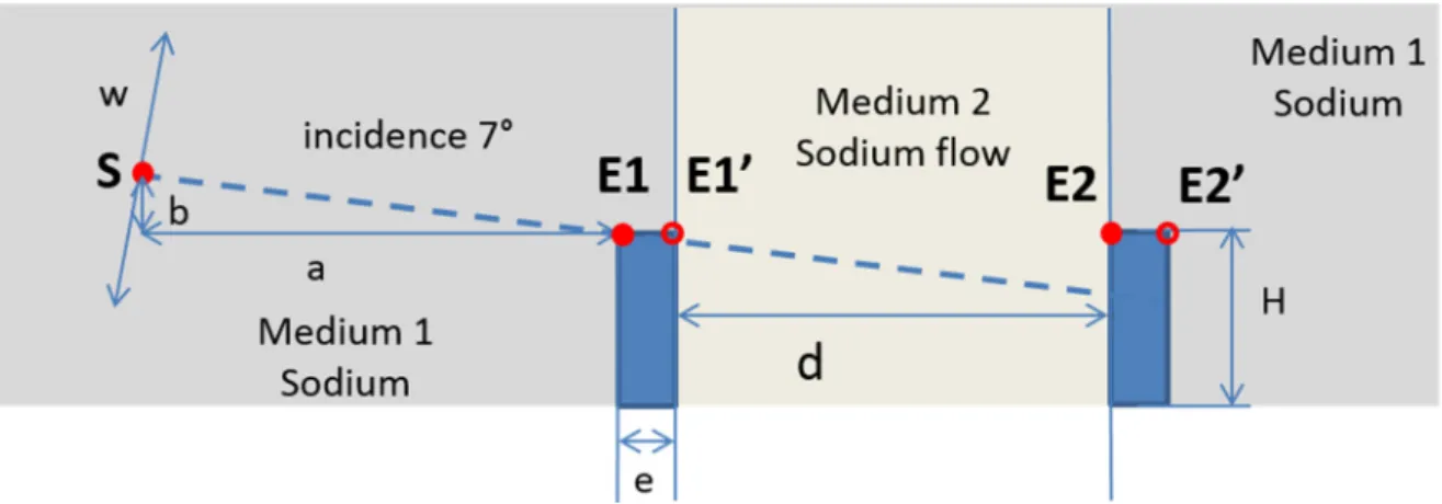
Figure 1 describes the 2D geometry that we consider. We model a transducer source (S) using a line of acoustic point sources of width w. We define a setup with grazing incidence of about 7° because measurements performed in water in previous work gave good experimental results in such a configuration [26]. The solid (stainless steel) tube representing the fuel assembly has an inner diameter d of 100 mm. The thickness e of the tube is 13 mm. Echoes will arrive from edges E1 and E2, and possibly from edges E1’ and E2’ as well. We will measure time differences between the main echoes E1 and E2.
Figure 1. Ultrasonic thermometry configuration used in our study.
3. Spectral-element numerical simulation in the context of ultrasonic
waves
We use a Legendre spectral-element method (SEM) in the time domain to discretize and solve the acoustic wave propagation equation. The SEM is an accurate and efficient technique to numerically model acoustic or seismic wave propagation, as it combines the
flexibility of finite-element techniques with the high accuracy of pseudospectral methods (see e.g. [18,19] and references therein). It is based on the weak form of the equations of motion rather than on their strong (i.e., differential) form and thus belongs to the family of Continuous Galerkin finite-element methods. It is highly efficient both on serial and on large parallel computers owing to its tensorized basis functions and a perfectly diagonal mass matrix [20,21]. We select this technique because it has been shown, for instance in geophysics [18,19,22], that it is very accurate for acoustic and seismic wave propagation problems, having very low numerical dispersion, and that it can accurately and efficiently handle meshes designed for complex geometries [20,21]. Smooth wave speed gradients inside the elements of the mesh as well as fluid-solid interfaces [20] can be accounted for, as also shown recently in ocean acoustics [23]. This will enable us to accurately compute the effects of temperature gradients on the acoustic echoes coming from the geometry of the tubes.
In that spectral-element technique, time integration is usually performed based upon an explicit Newmark time scheme [24]. Such a scheme is conditionally stable, i.e. the time step must remain below a threshold value for the time integration scheme to remain stable, with a stability condition,
(3) where cp is pressure wave velocity in the medium and α 0.50 the so-called Courant number
of the scheme [24].
We use the open-source SPECFEM software package [23] to perform these spectral-element numerical simulations of wave propagation.
4. Numerical simulations
We consider the framework of an effective medium to model the propagation medium. Density and wave velocity of the background model are modified to incorporate the effects of a heterogeneous medium due to the sodium flow, which only implies temperature gradients. Three conditions have to be met to validate the hypothesis of linear behavior as well as plane (or quasi-plane) wave propagation [25]:
- the deviation of the beam must remain weak,
- the gradient of the flow velocity relative to the Mach number must remain moderate, - the typical size of the heterogeneities must be large compared to the acoustic
wavelength.
These three conditions were verified and shown to apply in the cases under study in another study based on a ray-tracing code [8] and on the analysis of real thermohydraulic data [26]. Characteristic sizes of flow heterogeneities, typically ranging between 0.1 cm and 10.0 cm, are also large compared to the wavelengths of the ultrasonic waves considered [12].
As the measurement area is located just above the outlet of the fuel assembly, the flow is relatively regular and with smooth variations only and high Reynolds number. In such a case ultrasonic wave propagation is mainly affected by temperature distribution in the flow, and in our study we can therefore neglect the effects of the speed of the flow. The assumption of an effective medium is thus valid and the propagation medium can then simply be described by its density and the bulk modulus of the fluid, without having to explicitly model the fluid flow.
The study of the PLAJEST experiment of mixing cold and hot sodium flows [27], and its detailed numerical simulation at the French Atomic Commission using the TrioU code [28] leads us to choose a continuous parabolic variation of temperature inside the jet. Regarding the possible presence of microbubbles, there are not enough data for future reactors to currently be able to take this parameter into account. Doing so will require a complete study,
as the influence of the presence of such microbubbles will depend on bubble sizes as well as on transducer frequency [9]. The relation between ultrasonic velocity and temperature is given by equation (1), and equation (2) gives the density of sodium as a function of temperature T in Kelvin.
In order to perform our spectral-element simulations, we first create a mesh of the structure under study using the ‘Gmsh’ mesh creation tool [29]. The mesh created is entirely composed of quadrangles, as required by the spectral-element technique. Around the region of interest we resort to an absorbing boundary layer called the Perfectly Matched Layer (PML, [30,31]) in order to efficiently absorb the outgoing wave field; we use three layers of spectral elements on the outer edges of the mesh in order to implement it. The computational domain has a size of 723 mm (width) by 156 mm (height) and contains 448,704 elements. We use a polynomial degree N = 4 to define the basis functions in the spectral-element method, thus each spectral element contains (N + 1)2 = 25 grid points and the total number of unique grid
points is 7,108,112. Considering the sound velocity in liquid sodium at 450℃ (2339 m/s) and a dominant frequency of the ultrasonic source of 1 MHz, the number of grid points per shortest wavelength in the medium is thus approximately 4.7. We simulate a total physical time of 202.5 µs using a time discretization step of 7.5 × 10⁻9 s, i.e., a total of 27,000 time
steps
To speed up the calculations we resort to parallel computing on a cluster of computers [21,30]. Once the mesh is created we thus partition it according to the number of processor cores to be used for the calculation. Each processor core then carries out the calculations in a subdomain, and the results are recombined at the end of each time step of the time-stepping algorithm. We perform our calculations using 128 processor cores.
We select the location to use for the ultrasonic source (S) based on the position of point E1 and on distances a and b in Figure 1. Values of a and b equal to 100 mm and 12 mm lead to an incidence angle of 7°. To simulate the behavior of the transducer and create a quasi-plane wave of finite extension we sum 1000 point sources using a Hamming apodization function over a total width of about 67.6 mm. Each point source has a Ricker (i.e., the second derivative of a Gaussian) wavelet time function with a dominant frequency of 1 MHz [23]. The height of the upper part of the stainless steel tube is 50 mm, its thickness is 13 mm and its inner diameter is 100 mm.
The ratio between the known propagation distance and the time-of-flight difference between echoes E2 and E1 enables us to estimate the velocity of sound and then, based on equation (1), the mean temperature of the sodium flow on the outer edge of the tube.
4.3 Temperature variations studied
As stated above the propagation medium is in a turbulent state and its temperature distribution varies in a complicated fashion both in space and in time between, inside and above the assembly edges. Buffet [32], Fiorina [10] and Lü [12] have studied wave propagation in a turbulent liquid metal flow and, regarding sound velocity in such a medium, have decomposed the medium into two parts: a heterogeneous static part, and a random fluctuation part caused by the turbulent flow. In our study we will first perform simulations in the presence of a static temperature distribution only, and then in a second step with temperature fluctuations in the whole propagation region, generated based on a Gaussian random field.
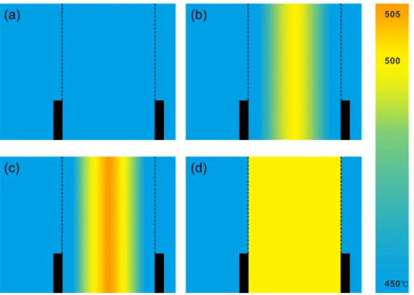
Figure 2. The four types of static temperature fields that we will use in our study: (a) T450, (b) TVAR, (c) TVAR+5, (d) T500. They differ only between the two edges of the outlet (vertical dotted lines). Model T450 has a constant temperature of 450 everywhere, TVAR has a parabolic variation from 450 to 500 between the two assembly edges, TVAR+5 has a parabolic variation from 450 to 505 , and T500 has a constant temperature of 500 between the two edges and of 450 outside.
4.3.1 Static temperature fields
As shown in Figure 2 we select four simple static temperature distributions in and at the outlet of the tube (called “medium 2” in the following) as well as in the surrounding sodium (called “medium 1”). In the first temperature profile (T450) we consider a homogeneous medium with a constant temperature of 450°C in both medium 1 and medium 2. It will be our reference case. In the second profile (TVAR) we consider a gradual evolution of temperature in medium 2, using a symmetric parabolic profile varying from 450°C to
500°C between the edge and the axis of the tube. Medium 1 still has a constant temperature of 450°C. In the third profile (TVAR+5) we use the same kind of profile as in the second but with an increase of 5°C, i.e., about 1%, of the maximum temperature in medium 2 only. The parabolic profile thus varies from 450°C to 505°C. In the fourth profile (T500) we finally consider a simplified temperature model of 500°C everywhere in the tube and at its outlet (medium 2) and 450°C everywhere in medium 1.
In these four cases the arrival time of the first echo does not vary, since medium 1 is unchanged. We thus focus our analysis on the variations of the second echo (wave reflection at point E2 in Figure 1).
4.3.2 Temperature fluctuation using a Gaussian random field
Gaussian random fields have been developed for digital simulation of multivariate, multidimensional, or multivariate-multidimensional random processes. They are used for instance in numerical analysis of nonlinear structures, numerical solution of stress wave propagation through a random medium, and eigenvalue problems of structures that have random homogeneous properties. Here we create Gaussian random fields for the fluctuation of the temperature field given by
1 1
1 (4)
where is temperature at the spatial position , is given by each of the static temperature profiles defined in Figure 2, and is the fluctuation part calculated by the Gaussian random field.
Following work on wave propagation in turbulent media (e.g. Lü [12]) we define the randomness of the temperature fluctuation as an isotropic homogeneous random field by a series cosine functions, expressing as:
√2 ∑ cos ∙ , (5) where k is the mode number and N is the total number of modes. is the wave vector, its angle from a coordinate axis of the wave vector of each mode is cos | |, and its modulus | | is defined by 1 , linearly distributing it in the range , . is the wave vector increment. For this process two random input values and are necessary: is distributed uniformly and randomly in 0
2 . Hence its probability density function Pr from 0 to 2 is Pr 0 2 1/2 . The other random variety is also uniformly distributed in 0 . is the spectral density function and is calculated based on the autocorrelation function as:
, (6)
where is the magnitude of the position vector (i.e. | |). For a Gaussian random field, the autocorrelation function is defined by a Gaussian distribution following the central limit theorem:
/ , (7)
with the covariance, the autocorrelation function, the variance of the random value, and the characteristic length of the random pattern. R is the distance between two different points ( , ) in the region in which the random field is simulated, i.e., | |.
After applying a Fourier transform to equation (6) the spectral density function then writes:
We use typical values from the NAJECO experiment [26] to choose the characteristic length 0.03 m. We set the standard deviation of the fluctuation to 0.029 to be able to generate a maximum difference of about 30 degrees (Figure 3), following a thermohydrodynamic calculation result obtained at the French Atomic Commission [26]. The total number of modes N and the range of the wave vector modulus [ , ] need to be chosen carefully: N needs to be large enough to keep a sufficient data set because Equation (5) is asymptotically an exact expression for the covariance function when tends to infinity [14], and not doing so may introduce numerical errors [33]. The range , needs to be wide enough to express the entire curve of the spectral density function. After numerical tests and following a discussion about the minimum requirements of these values in [22] we select N = 64, 6/ , and . (The range of the wave vector needs to be symmetric because the spectral density function of the Gaussian process is symmetric).
We generate 30 different patterns of the fluctuation field, and thus obtain 30 temperature fields to be simulated by superimposing the fluctuation field with the static temperature field based on Equation (4). Figure 3 shows the distribution of the magnitude, defined as the difference with the average temperature (450 ), of the temperature fluctuation for all 30 fluctuation patterns.
Figure 3. Distribution of the 30 different temperature fluctuation fields. The magnitude of the fluctuation is defined as the difference with the average temperature calculated from all
fluctuation fields (450 ).
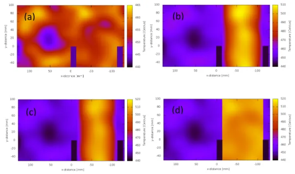
Figure 4 shows examples of such generated temperature fields. In the generation of the fluctuation field the origin point of (i.e., the coordinate of point ) in equation (4) is set at the upper-left corner of the nearest assembly edge. In Figure 4a the temperature scale is truncated to show the random patterns more clearly. The temperature changes in the vertical shapes along the sodium jet are due to the temperature profile (see Figure 2); they are right edges in the case of the rectangular profile (Figure 4d) and more variable edges in the case of a parabolic distribution (Figure 4b and 4c).
Figure 4. Examples of generated fluctuating temperature fields obtained when using the (a) T450, (b) TVAR, (c) TVAR+5 and (d) T500 temperature profiles of Figure 2.
(a)
(c)
(d)
We then carried out simulations of wave propagation in these models and calculated times of flight in the 120 resulting patterns of the temperature field, constructed by overlaying the 30 Gaussian random field patterns with each of the four types of static temperature profile, as we will describe in the next section.
5. Results and discussion
5.1 Results with static temperature fields
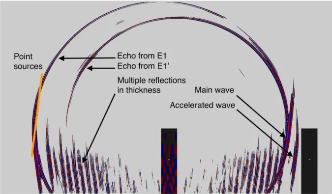
In Figure 5 we show the pressure of the acoustic wave in the computational domain normalized between -1 (blue) and +1 (red), with color intensity obeying a power law with exponent 0.3 in order to significantly enhance small values for visualization purposes. Such a nonlinear color scale amplifies the real amplitude of the minor echoes such as the second diffraction E1’ in order to observe them more easily. All amplitudes below 1% are discarded in order to avoid visually amplifying very small-amplitude numerical noise. Figure 5 highlights several aspects of wave propagation near the upper part of the fuel assembly. The waves diffracted from edges E1 and E1’ are both clearly observed.
The time t = 88.125 µs at which the figure is drawn allows us to observe the wave just before it interacts with the second point E2. Since the incidence angle is very small, the lower part of the wave front goes through the thickness of the tube with a much greater velocity (about 5.8 mm/µs in steel versus about 2.3 mm/µs in sodium) and is well seen as a small wave that propagates before the main one. Figure 5 also shows a superimposition of waves: the main wave and the wave diffracted from E1’. This illustrates the interest of such snapshots as well as movies of wave propagation in the time domain to facilitate signal analysis and identification of wave fronts in such applications.
Figure 5. Snapshot of wave propagation at time t = 88.125 µs simulated using our spectral-element numerical modeling technique; we display the pressure variation field (blue being
negative and red positive).
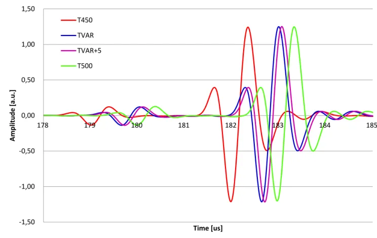
Figure 6 shows the signals recorded at point S of Figure 1 for a time window that allows us to observe the signal reflected off the second edge (point E2) for the four different temperature configurations. These signals are recorded when the waves come back to the source, i.e. in the so-called echo mode in non-destructive testing. As wave velocity decreases when sodium temperature increases (Equation 1), the signal is delayed when temperature increases. The respective time delays of the four signals are qualitatively in agreement with the expected behavior: the hotter medium 2 is, the larger the delay for the time-of-flight from point E2 is as well. We observe a small time difference when the parabolic temperature distribution is increased by 5°, i.e., by about one percent. The small accelerated wave observed in Figure 5 leads to a weaker signal that arrives before the main echo around time t = 179 µs. This signal is 20 dB lower than the maximum signal because this part of the beam underwent transmission through steel; in practice in a real experimental setup it could thus be
masked by signal noise. Both of these signals are due to the waves diffracted off point E2. As the duration of the wave corresponds to about two periods, similar to a highly damped transducer, no interferences occur between these two waves; this can also be seen in Figure 5, in which the waves are clearly separated.
Figure 6. Comparison between the echoes reflected off point E2 in the four simulations performed for the model with right-angle edges.
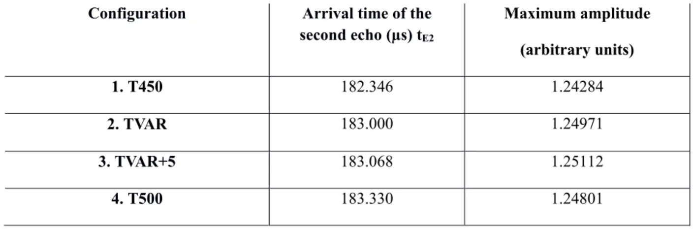
In order to perform a more quantitative analysis, in Table 1 we give the arrival times in µs of the second echo measured at the signal maximum. Corresponding pressures have arbitrary units because, since the wave equation is linear, the amplitudes of the signals do not significantly vary and thus amplitude cannot be used to detect temperature variations in this configuration; we thus analyze arrival times only in our study.
‐1,50 ‐1,00 ‐0,50 0,00 0,50 1,00 1,50 178 179 180 181 182 183 184 185 Amplitude [a.u.] Time [us] T450 TVAR TVAR+5 T500
Configuration Arrival time of the second echo (µs) tE2 Maximum amplitude (arbitrary units) 1. T450 182.346 1.24284 2. TVAR 183.000 1.24971 3. TVAR+5 183.068 1.25112 4. T500 183.330 1.24801
Table 1. Time-of-flight and amplitude of the echo coming back from point E2 for the four
different temperature configurations in the case of a right-angle geometry.
The changes in the time-of-flight of the second echo at point E2 provide information on the ability and sensitivity of the method to detect small temperature variations in the case of the absence of temperature fluctuation. Between Simulations 2 and 3 we find that the increase of 5°C of the maximum of the temperature profile leads to a shift of 68 ns. As the time of flight of echo E1 is always the same, this difference is also the difference between the
times of flight of the echoes on the two edges (tE2 - tE1). In a reactor such a time difference
could be measured using a 1 MHz signal, i.e., a short signal, but that would require good signal-to-noise ratio and signal stability.
5.2 Results with temperature fluctuation
5.2.1 Effect of temperature fluctuation on time-of-flight
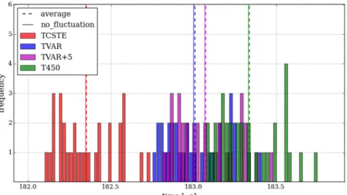
Let us now study the fluctuation in times of flight when temperature fluctuations in the medium are taken into account and see if it is still possible to detect such short time differences. We simulate wave propagation for 30 random temperature fields added to each of the four static fields, leading to a total of 120 different propagation media, and obtain
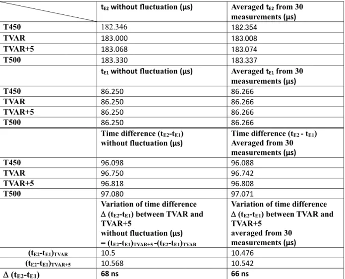
fluctuations of the time of flight for echo E2 but also for echo E1. We thus consider that the fluctuating media introduce a random noise around the true time of flight corresponding to a static situation. Figure 7 shows the resulting distribution of time of flight tE2 for the four static temperature cases. We observe an overlapping of various times of flight. An averaging procedure would be necessary to reconstruct the true time of flight as defined above. Table 2 summarizes time of flight measurements for both the E1 and E2 echoes without fluctuations (left column) and using averaged times of flight in the case of stochastic fluctuations (right
column). We then calculate the time difference between the two echoes (tE2 - tE1), as this
variation of the time difference would be a signature of variation in the sodium jet. The 5°C
difference between the two parabolic profiles TVAR and TVAR+5 creates a 68 ns difference between the times of flight difference from edges E2 and E1. This time difference is equal to about 66 ns when an average process is performed over 30 fluctuating temperature field.
Figure 7. Distributions of variation of times of flight resulting from temperature fluctuations for each of the 120 temperatures profiles considered, i.e. the 30 random profiles superimposed to each of the four static temperature profiles.
Table 2. Variations of time of flight between results for the cases without temperature fluctuations and averaged results from 30 measurements in cases with fluctuations.
tE2 without fluctuation (µs) Averaged tE2 from 30 measurements (µs)
T450 182.346 182.354
TVAR 183.000 183.008
TVAR+5 183.068 183.074
T500 183.330 183.337
tE1 without fluctuation (µs) Averaged tE1 from 30 measurements (µs) T450 86.250 86.266 TVAR 86.250 86.266 TVAR+5 86.250 86.266 T500 86.250 86.266 Time difference (tE2-tE1) without fluctuation (µs) Time difference (tE2 - tE1) Averaged from 30 measurements (µs) T450 96.098 96.088 TVAR 96.750 96.742 TVAR+5 96.818 96.808 T500 97.080 97.071
Variation of time difference (tE2-tE1) between TVAR and TVAR+5
without fluctuation (µs) = (tE2-tE1)TVAR+5 -(tE2-tE1)TVAR
Variation of time difference (tE2-tE1) between TVAR and TVAR+5 averaged from 30 measurements (µs) (tE2-tE1)TVAR 10.5 10.476 (tE2-tE1)TVAR+5 10.568 10.542 (tE2-tE1) 68 ns 66 ns
5.2.2 Detection of variations of statistic temperature by averaging
In Figure 8 we perform a more complete statistical analysis. If we calculate the standard deviation of time-of-flight measurements due to the random pattern in the temperature fields we can evaluate the probability of success to separate times of flight for a 1% temperature difference, i.e., 5°C in our case. In Table 2 we find that the variation in the
time-of-flight difference (tE2-tE1) between echoes E2 and E1 is 68 ns in the case of static
temperature fields; Considering classical Gaussian statistics, it is possible to statistically
standard deviation of the time-of-flight measurements is lower than 34 ns (2σ). To improve the chance of success the standard deviation should be lower than 17 ns (4σ) to separate times of flight with 95,45% of success, and lower than 11,33 (6σ) ns to separate times of flight with 99,73% of success. Figure 8 shows that these levels of confidence are reached when using respectively 15, 24 and 28 measurements.
Figure 8. Variation of the standard deviation of the mean time-of-flight with respect to the number of times-of-flight used to calculate the mean value.
6. Conclusions and future work
We have presented a 2D numerical modeling study based on a spectral-element method in the time domain to analyze variations of time of flight due to temperature changes in a fluid medium. We have shown that our numerical approach can accurately model the principle of ultrasonic thermometry above the core of a Sodium cooled Fast Reactor. Based on
our numerical approach we have illustrated the sensitivity of an ultrasonic thermometry method to a relatively weak temperature change. In the simulations with a static temperature profile we have shown that a temperature variation of about 1% of the average temperature could be detected, as this temperature variation induces a time shift of about 68 ns.
We generated 120 patterns of temperature fields using a Gaussian random field and examined their effect on the time-of-flight of the signal reflected off the assembly edges. We investigated the effect of temperature fluctuations on the variations of times-of-flight for four different patterns of static temperature profiles. Under these thermodynamically and acoustically complex conditions we found that it may be difficult to detect a 5-degree i.e. one percent variation in the static temperature field based on a single measurement, but also showed that by averaging times-of-flight coming from about 30 measurements such detection becomes possible with a high level of confidence.
In this study, we have considered that the void fraction (i.e., small free bubbles within the sodium) was negligible or stable, as can be expected in normal monitoring conditions. The measurement of the void fraction and its influence on sound velocity is ongoing in our group and its contributions to ultrasonic temperature measurement should thus be introduced in future studies. We have also considered ideal and perfectly-known geometrical conditions; In a real reactor some variations may occur, such as small assembly head shifts or bowing (irradiation-induced effect), which can modify the apparent diameter of the assembly for instance. However, these effects are small and vary very slowly with time during the monitoring periods, thus one can reasonably consider that they have no influence on the measurement of assembly outlet temperature variations.
We have taken the thermal static heterogeneity of the medium into account by considering a simplified medium and superimposing fluctuations created based on a random field generator. In future work we plan to extend our simulations to take into account a more
realistic medium defined based on the PLAJEST experimental data [27] or using computational fluid dynamics results of studies for new reactor designs that are currently being performed in a project called ASTRID (Advanced Sodium Technological Reactor for Industrial Demonstration) [34]. Taking flow rates i.e. a moving fluid into account will also require further development of our spectral-element technique. In addition to using a more complete description of liquid sodium above the fuel assemblies, further studies should also focus on better understanding the origin of signal noise to understand which part could be produced by medium fluctuations such as eddies or vortices. The results that we have obtained can be useful for ultrasonic thermometry, but our conclusions should also be valid for telemetry applications in which time-of-flight measurements are used to accurately locate objects in a liquid medium.
We adhere to the principles of reproducible research: The SPECFEM2D software package that implements our spectral-element numerical modeling technique is available open source from www.geodynamics.org.
Acknowledgements: The authors thank Paul Cristini for fruitful discussion about the
Hamming apodization function. Part of this work was funded by the Simone and Cino del Duca / Institut de France / French Academy of Sciences Foundation under grant #095164 and by the European `WAVES: Waves and Wave-Based Imaging in Virtual and experimental Environments' #641943 project of call H2020-MSCA-ITN-2014.
References
[1] Use of fast reactors for actinide transmutation, IAEA TEC-DOC 693 report, Vienna, Austria, IAEA publication, ISSN 1011-4289, 1993.
[2] H. Abderrahim, P. Kupschus, E. Malambu, P. Benoit, K. Van Tichelen, B. Arien, F. Vermeersch, P. D’hondt, Y. Jongen, S. Ternier, D. Vandeplassche, MYRRHA: A multipurpose accelerator driven system for research and development. Nuclear Instruments and methods in physics research. vol. 463, p. 487–494, 2001.
[3] T. Abram, S. Ion, Generation-IV nuclear power: A review of the state of the science, Energy Policy vol. 36, p. 4323-4330, 2008.
[4] J. P. Jeannot, G. Rodriguez, C. Jammes, B. Bernardin, J. L. Portier, F. Jadot, S. Maire, D. Verrier, F. Loisy, G. Préle, Research and Development Program for Core Instrumentation Improvements Devoted for French Sodium-Fast Reactors, ANIMMA Conference, Marseille, France, 2011.
[5] J. L. Berton, G. Loyer, Continuous Monitoring of the Position of two Subassemblies Heads of Phénix at 350 MWth Power and 550°C Temperature, SMORN VII Conference, 19-23 June, Avignon, France, 1995.
[6] J. Daw, J. Rempe, S. Taylor, J. Crepeau, S. Curtis Wilkins, Ultrasonic Thermometry for In-Pile Temperature Detection, Seventh American Nuclear Society International Topical Meeting on Nuclear Plant Instrumentation, Control and Human-Machine Interface Technologies, NPIC & HMIT 2010, Las Vegas, Nevada, USA, November 7-11, 2010.
[7] J. A. McKnight, I. D. Macleod, E. J. Burton, Remote temperature measurement, patent number 4 665 992, 1987.
[8] N. Massacret, J. Moysan, M. A. Ploix, J. P. Jeannot and G. Corneloup, Modelling of ultrasonic propagation in turbulent liquid sodium with temperature gradient, Journal of Applied Physics vol. 115(20), p. 204905-204905-8, 2014.
[9] M. Cavaro, C. Payan, J. Moysan, F. Baque, Microbubble cloud characterization by nonlinear frequency mixing, Journal of the Acoustical Society of America, vol. 129(5), p. E179-E189, 2011.
[10] D. Fiorina, Application de la méthode de sommation de faisceaux gaussiens à l'étude de la propagation ultrasonore en milieu turbulent, Ph.D. thesis, École Centrale de Lyon, France, 1999.
[11] C. Lhuillier, D. Fiorina, D. Juvé, Simulation of ultrasound propagation in a thermally turbulent fluid using Gaussian beam summation and Fourier modes superposition techniques, 16th ICA, 20-26th June 1998, Seattle, USA.
[12] S. Grewal, E. Gluekler, Water simulation of sodium reactors, Chem. Eng. Comm., Vol. 17, pp 343-360, 1982.
[13] B. Lü, M. Darmon, C. Potel, Stochastic simulation of the high-frequency wave propagation in a random medium, J. Appl. Phys. vol. 112, p. 054902, doi: 10.1063/1.4748274, 2012.
[14] M. Shinozuka, Digital simulation of random processes and its applications, J. Sound Vib., 25(1), p.111-128, 1972.
[15] V. Sobolev, Database of thermophysical properties of liquid metal coolants for GEN-IV, SCK-CEN, Scientific Report BLG-1069, November 2010, Mol, Belgium.
[16] Y. Liu, G. Du, L. Tao and F. Shen, The calculation of the profile-linear average velocity in the transition region for ultrasonic heat meter based on the method of LES, Journal of hydrodynamics, vol. 23(1) pp.89-94, 2011.
[17] F. J. Weber, Ultrasonic Beam Propagation in Turbulent Flow, Ph.D. thesis, Worcester Polytechnic Institute, Worcester, Massachusetts, USA, 2003.
[18] J. Tromp, D. Komatitsch, Q. Liu, Spectral-Element and Adjoint Methods in Seismology, Communication in Computational Physics, vol. 3(1), p. 1-32, 2008.
[19] R. Vai, Castillo-Covarrubias, J. M.; Sánchez-Sesma, F. J.; Komatitsch, D. and Vilotte, J. P., Elastic wave propagation in an irregularly layered medium, Soil Dynamics and Earthquake Engineering, vol. 18, p. 11-18, 1999.
[20] D. Komatitsch, Fluid-solid coupling on a cluster of GPU graphics cards for seismic wave propagation, Comptes Rendus de l'Académie des Sciences – Mécanique, vol. 339, p. 125-135, doi: 10.1016/j.crme.2010.11.007, 2011.
[21] D. Peter, Dimitri Komatitsch, Y. Luo, R. Martin, N. Le Goff, E. Casarotti, P. Le Loher, F. Magnoni, Q. Liu, C. Blitz, T. Nissen-Meyer, P. Basini and J. Tromp, Forward and adjoint simulations of seismic wave propagation on fully unstructured hexahedral meshes, Geophysical Journal International, vol. 186(2), p. 721-739, doi: 10.1111/j.1365-246X.2011.05044.x, 2011.
[22] S.-J. Lee, D. Komatitsch, B.-S. Huang and J. Tromp, Effects of topography on seismic wave propagation: An example from northern Taiwan, Bulletin of the Seismological Society of America, vol. 99(1), p. 314-325, doi: 10.1785/0120080020, 2009.
[23] P. Cristini and D. Komatitsch, Some illustrative examples of the use of a spectral-element method in ocean acoustics. Journal of Acoustical Society of America, vol. 131(3), p. EL229-EL235, 2012.
[24] T. J. R. Hughes, The finite element method, linear static and dynamic finite element analysis, Prentice-Hall International, 1987.
[25] O. Godin, An effective quiescent medium for sound propagating through an inhomogeneous, moving fluid, Journal of Acoustical Society of America, vol. 112(4), p. 1269-1275, 2002.
[26] D. Tenchine, Some thermal hydraulic challenges in sodium cooled fast reactors, Nuclear Engineering and Design, vol. 240(5), p. 1195-1217, 2010.
[27] N. Kimura, H. Miyakoshi and H. Kamide, Experimental investigation on transfer characteristics of temperature fluctuation from liquid sodium to wall in parallel triple jet, International Journal of Heat and Mass Transfer, vol. 50, p. 2024-2036, 2006.
[28] G. Brillant., F. Bataille, F. Ducros, Large-eddy simulation of a turbulent boundary layer with blowing, Theoretical and Computational Fluid Dynamics, vol. 17(5-6), p.433-443, 2004. [29] C. Geuzaine and J.-F. Remacle. Gmsh: a three-dimensional finite element mesh generator with built-in pre- and post-processing facilities, International Journal for Numerical Methods in Engineering, vol. 79(11), p. 1309-1331, 2009.
[30] R. Martin, D. Komatitsch, S. D. Gedney, A variational formulation of a stabilized unsplit convolutional perfectly matched layer for the isotropic or anisotropic seismic wave equation, Computer Modeling in Engineering and Sciences, vol. 37(3), p. 274-304, 2008.
[31] R. Martin, D. Komatitsch, An unsplit convolutional perfectly matched layer technique improved at grazing incidence for the viscoelastic wave equation, Geophysical Journal International, vol. 179(1), p. 333-344, doi: 10.1111/j.1365-246X.2009.04278.x, 2009.
[32] J. C. Buffet, Étude des fluctuations de température dans des écoulements de métal liquide au voisinage d'une paroi, Ph.D. thesis, École Centrale de Lyon, France, 1984.
[33] A. Mantoglou and J. L. Wilson, The Turning Bands Method for Simulation of Random Fields Using Line Generation by a Spectral Method, Water Resour. Res., vol. 18, no. 5, pp. 1379–1394, 1982.
[34] P. Le Coz, J. F. Sauvage, J. P. Sepantie, Sodium-cooled fast reactors: the ASTRID plant project, Proceedings of the ICAPP 2011 conference, 2-6 May 2011, Nice, France, 2011.