HAL Id: hal-02873740
https://hal.inria.fr/hal-02873740
Submitted on 18 Jun 2020
HAL is a multi-disciplinary open access
archive for the deposit and dissemination of
sci-entific research documents, whether they are
pub-lished or not. The documents may come from
teaching and research institutions in France or
abroad, or from public or private research centers.
L’archive ouverte pluridisciplinaire HAL, est
destinée au dépôt et à la diffusion de documents
scientifiques de niveau recherche, publiés ou non,
émanant des établissements d’enseignement et de
recherche français ou étrangers, des laboratoires
publics ou privés.
Jean-Daniel Boissonnat, Siddharth Pritam
To cite this version:
Jean-Daniel Boissonnat, Siddharth Pritam. Edge Collapse and Persistence of Flag Complexes. SoCG
2020 - 36th International Symposium on Computational Geometry, Jun 2020, Zurich, Switzerland.
�10.4230/LIPIcs.SoCG.2020.19�. �hal-02873740�
Jean-Daniel Boissonnat
Université Côte d’Azur, INRIA, Sophia Antipolis, France Jean-Daniel.Boissonnat@inria.fr
Siddharth Pritam
Université Côte d’Azur, INRIA, Sophia Antipolis, France siddharth.pritam@inria.fr
Abstract
In this article, we extend the notions of dominated vertex and strong collapse of a simplicial complex as introduced by J. Barmak and E. Miniam. We say that a simplex (of any dimension) is dominated if its link is a simplicial cone. Domination of edges appears to be a very powerful concept, especially when applied to flag complexes. We show that edge collapse (removal of dominated edges) in a flag complex can be performed using only the 1-skeleton of the complex. Furthermore, the residual complex is a flag complex as well. Next we show that, similar to the case of strong collapses, we can use edge collapses to reduce a flag filtration F to a smaller flag filtration Fcwith the same persistence. Here again, we only use the 1-skeletons of the complexes. The resulting method to compute Fcis simple and extremely efficient and, when used as a preprocessing for persistence computation, leads to gains of several orders of magnitude w.r.t the state-of-the-art methods (including our previous approach using strong collapse). The method is exact, irrespective of dimension, and improves performance of persistence computation even in low dimensions. This is demonstrated by numerous experiments on publicly available data.
2012 ACM Subject Classification Mathematics of computing; Theory of computation → Computa-tional geometry; Mathematics of computing → Topology
Keywords and phrases Computational Topology, Topological Data Analysis, Edge Collapse, Simple Collapse, Persistent homology
Digital Object Identifier 10.4230/LIPIcs.SoCG.2020.19
Funding This research has received funding from the European Research Council (ERC) under the European Union’s Seventh Framework Programme (FP/2007- 2013) / ERC Grant Agreement No. 339025 GUDHI (Algorithmic Foundations of Geometry Understanding in Higher Dimensions).
Acknowledgements We want to thank Marc Glisse for useful discussions and Vincent Rouvreau for his help with Gudhi.
1
Introduction
Improving the performance of computing persistent homology has been a central goal in Topological Data Analysis (TDA) since the early days of the field about 20 years ago. Very significant progress has been obtained on the two main components of the overall pipeline: the preprocessing of the sequence of complexes given as input and the computation of persistence homology (PH). The latter line of research led to improvement of the persistence algorithm and of its analysis, to efficient implementations and optimizations, and to a new generation of software [37, 8, 6, 45]. The former and complementary direction has been intensively explored with the goal of reducing the size of the complexes in the input sequence while preserving the persistent homology of the sequence, or approximating it in a controlled way [44, 30, 18, 13, 51, 41, 20, 27]. Among the most widely used complexes in TDA are the flag complexes and, in particular, the Vietoris-Rips complexes. These complexes are of great theoretical and practical interest since they are fully characterized by their graph (or 1-skeleton) and can thus be stored in a very compact way. Specific algorithms and very
© Jean-Daniel Boissonnat and Siddharth Pritam; licensed under Creative Commons License CC-BY
efficient codes have been developed for those complexes [6, 51]. Despite all these advances, further progress has been obtained recently both for general simplicial complexes [12] and for flag complexes [11] using a special type of collapses, called strong collapses, introduced by J. Barmak and E. Miniam [5]. The basic idea is to simplify the complexes of the input sequence by using strong collapses and to compute the PH of an induced sequence of reduced simplicial complexes whose PH is the same or a close approximation of the PH of the initial sequence. In the case of flag complexes, the critical observation was that the construction of the reduced sequence can be done using only the 1-skeletons of the complexes, without constructing the full complexes, therefore saving time and space.
This paper further improves on these last results. Although the general philosophy is the same, there are some new key features that make the new method several orders of magnitude more efficient than all known methods.
1. Instead of strong collapses, we use the so-called edge collapses. In fact, we more generally define k-collapses that are identical to the extended collapses introduced in [4] (see also the early work of V. Welker [53]). When k = 0, we have strong collapses and when k = 1 edge collapses. Edge collapses share with strong collapses some important properties. Most notably, we can use edge collapses to reduce any flag filtration F to a smaller flag filtration Fc with the same persistence, using only the 1-skeletons of the complexes.
2. The reduction is exact and the PH of the reduced sequence is identical to the PH of the input sequence. However, the method can be easily adapted so as to produce an approximate reduction that would lead to better run time.
3. In [12] and in [11], the reduced sequence associated to a filtration was usually a tower (a sequence of simplicial complexes connected through simplicial maps), and part of the computing time was devoted to transforming this tower in another equivalent filtration using ideas from [26, 40]. There is no such need in the algorithm presented in this paper, which is another main source of improvement. Note however that the algorithm described in [11] works for flag towers while, in this paper, we restrict ourselves to flag filtrations.
4. The resulting method is simple and extremely efficient. On the theory side, we show that the edge collapse of a flag filtration can be computed in time O(n nck2), where n and
nc are the number of edges in the input and output 1-skeletons respectively and k is the
maximal degree of a vertex in the input graph. The algorithm has been implemented. Numerous experiments on publicly available data show that preprocessing PH computation of flag complexes using edge collapse leads to unprecedented performance. The code will be soon released in the Gudhi library [37].
An outline of this paper is as follows. Section 2 recalls some basic ideas and constructions related to simplicial complexes and simple collapses. We introduce k-collapses and then edge collapses in Section 3. In Section 4, we prove that simple collapses preserve persistence. In Section 5, we provide the main algorithm that reduces a flag filtration to another flag filtration using edge collapses. Experiments are discussed in Section 6.
2
Preliminaries
In this section we provide some background material. Readers can refer to [38] for a comprehensive introduction to these topics.
Simplex, simplicial complex and simplicial map. An abstract simplicial complex K is a collection of subsets of a non-empty finite set X, such that for every subset A in K, all the subsets of A are in K. From now on, we will call an abstract simplicial complex simply
a simplicial complex or just a complex. An element of K is called a simplex. An element of cardinality k + 1 is called a k-simplex and k is called its dimension. Given a simplicial complex K, we denote its geometric realization as |K|. A simplex is called maximal if it is not a proper subset of any other simplex in K. A sub-collection L of K is called a subcomplex if it is a simplicial complex itself.
A map ψ : K → L between two simplicial complexes is called a simplicial map if it always maps a simplex in K to a simplex in L. Simplicial maps are induced by vertex-to-vertex maps. A simplicial map ψ : K → L between two simplicial complexes K and L induces a continuous map |ψ| : |K| → |L| between the underlying geometric realizations. Any general simplicial map can be decomposed into more elementary simplicial maps, namely elementary inclusions (i.e., inclusions of a single simplex) and elementary contractions {{u, v} 7→ u} (where a vertex is mapped onto another vertex). The inverse operation of an
inclusion is called a simplicial removal, denoted as K ←- L.
Flag complex and Neighborhood. A complex K is a flag or a clique complex if, when a subset of its vertices form a clique (i.e. any pair of vertices is joined by an edge), they span a simplex. It follows that the full structure of K is determined by its 1-skeleton (or graph) we denote by G. For a vertex v in G, the open neighborhood NG(v) of v in G is defined as
NG(v) := {u ∈ G | [uv] ∈ E}, here E is the set of edges of G. The closed neighborhood
NG[v] is NG[v] := NG(v) ∪ {v}. Similarly we define the closed and open neighborhood of an
edge [xy] ∈ G, NG[xy] and NG(xy) as NG[xy] := N [x] ∩ N [y] and NG(xy) := N (x) ∩ N (y),
respectively. The above definitions can be extended to any k-clique σ = [v1, v2, ..., vk] of G;
NG[σ] :=Tvi∈σN [vi] and NG(σ) :=Tvi∈σN (vi).
Star, Link and Simplicial Cone. Let σ be a simplex of a simplicial complex K, the closed star of σ in K, stK(σ) is a subcomplex of K which is defined as follows, stK(σ) := {τ ∈
K| τ ∪ σ ∈ K}. The link of σ in K, lkK(σ) is defined as the set of simplices in stK(σ) which
do not intersect with σ, lkK(σ) := {τ ∈ stK(σ)|τ ∩ σ = ∅}. The open star of σ in K, stoK(σ)
is defined as the set stK(σ) \ lkK(σ). Usually stoK(σ) is not a subcomplex of K.
Let L be a simplicial complex and let a be a vertex not in L. Then the set aL defined as aL := {a, τ | τ ∈ L or τ = σ ∪ a; where σ ∈ L} is called a simplicial cone.
Sequences of complexes. A sequence of simplicial complexes T : {K1
f1
−→ K2
f2
−→ · · ·−−−−→ Kf(m−1) m} connected through simplicial maps fiis called a simplicial tower or simply
a tower. When all the simplicial maps fiare inclusions, the tower is called a filtration. If all
the simplicial complexes Ki are flag complexes, we call it flag towers and flag filtrations.
Persistent homology. If we compute the homology classes of all the Ki, we get the sequence
P(T ) : {Hp(K1) f1∗ −→ Hp(K2) f2∗ −→ Hp(K3) f3∗ −→ · · · f ∗ (m−1)
−−−−→ Hp(Km)}. Here Hp() denotes the
homology class of dimension p with coefficients from a field F and fi∗ is the homomorphism
induced from fi. P(T ) is a sequence of vector spaces connected through the fi∗ called a
persistence module. More formally, a persistence module V is a sequence of vector spaces {V1 −→ V2 −→ V3 −→ · · · −→ Vm} connected with homomorphisms {−→} between them. A
persistence module arising from a sequence of simplicial complexes captures the evolution of the topology of the sequence. Two different persistence modules V : {V1−→ V2−→ · · · −→ Vm}
and W : {W1−→ W2−→ · · · −→ Wm}, connected through a set of homomorphisms φi: Vi→ Wi
V1 V2 · · · Vm−1 Vm
W1 W2 · · · Wm−1 Wm
φ1 φ2 φm−1 φm
Any persistence module can be decomposed into a collection of intervals of the form [i, j) [14]. The multiset of all the intervals [i, j) in this decomposition is called the persistence diagram of the persistence module. An interval of the form [i, j) in the persistence diagram of P(T ) corresponds to a homological feature (a “cycle”) which appeared at i and disappeared at j. The persistence diagram (PD) completely characterizes the persistence module, that is, there is a bijective correspondence between the PD and the equivalence class of the persistence module [14, 58]. In other words, equivalent persistence modules have the same the same persistence diagram.
Simple collapse. Given a complex K, a simplex σ ∈ K is called a free simplex if σ has a unique coface τ ∈ K. The pair {σ, τ } is called a free pair. The action of removing a free pair: K → K \ {σ, τ } is called an elementary simple collapse. A series of such elementary simple collapses is called a simple collapse. We denote it as K & L. This operation preserves the homotopy type of the simplicial complex K, which we write K ∼ L. In particular, there is a retraction map |r| : |K| → |L| between the underlying geometric realization of K and L which is a strong deformation retraction. A complex K0 will be called simple-collapse minimal if there is no free pair {σ, τ } in K0. A subcomplex Kec of K is
called an elementary core of K if K&Kecand Kec is simple-collapse minimal.
Removal of a simplex. We denote by K \ σ the subcomplex of K obtained by removing σ, i.e. the complex that has all the simplices of K except the simplex σ and the cofaces of σ.
3
Edge Collapse
In this section, we first extend the definition of a dominated vertex introduced in [5] to simplices of any dimension. Given a simplex σ ∈ K, we denote by Σσ the set of maximal
simplices of K that contain σ. The intersection of all the maximal simplices in Σσ will be
denoted asT Σσ:=Tτ ∈Σστ .
Dominated simplex. A simplex σ in K is called a dominated simplex if the link lkK(σ)
of σ in K is a simplicial cone, i.e. if there exists a vertex v0 ∈ σ and a subcomplex L of K,/ such that lkK(σ) = v0L. We say that the vertex v0 is dominating σ and that σ is dominated
by v0, which we denote as σ ≺ v0.
k-collapse. Given a complex K, the action of removing a dominated k-simplex σ from K is called an elementary k-collapse, denoted as K&&k{K \ σ}. A series of elementary k-collapses is called a k-collapse, denoted as K &&k L. We further call a complex K k-collapse minimal if it does not have any dominated k simplices. A subcomplex Kk of
K is called a k-core if K &&k Kk and Kk is k-collapse minimal.
The notion of k-collapse is the same as the notion of extended collapse introduced in [4]. We give it a different name to indicate the dependency on the dimension. A 0-collapse is a strong collapse as introduced in [5]. A 1-collapse will be called an edge collapse. It is not hard to
see that an elementary simple collapse of a k-simplex σ is a k-collapse, as it is dominated by the vertex v = τ \ σ, where τ is the unique coface containing σ. Each k-collapse can be decomposed into a sequence of elementary simple collapses and therefore k-collapses preserve the simple homotopy type [53, Lemma 2.7] and [4, Lemma 8]. Therefore, like simple collapses, k-collapses induce a strong deformation retract as well on the geometric realization.
The following lemma extends a result in [5] to general k-collapse. It shows that the domination of a simplex can be characterized in terms of maximal simplices.
ILemma 1. A simplex σ ∈ K is dominated by a vertex v0 ∈ K, v0 ∈ σ, if and only if all/ the maximal simplices of K that contain σ also contain v0, i.e. v0∈T Σσ.
Proof. If σ ≺ v0 then lkK(σ) = v0L by definition. This implies that for any maximal simplex
τ in stK(σ), v0∈ τ . Therefore, v0∈T Σσ. For the reverse direction, let v0 ∈T Σσ. Hence,
for any maximal simplex τ in stK(σ), we have v0 ∈ τ . Now as v0 ∈ σ, v/ 0 belong to all the
simplices τ \ σ, and thus lkK(σ) = v0L where L = (τ \ σ) \ v0. Hence σ ≺ v0 iff v0∈T Σσ. J
Lemma 1 has important algorithmic consequences. To perform a k-collapse, one simply needs to store the adjacency matrix between the k-simplices and the maximal simplices of K.
Next we study the special case of a flag complex K and characterize the domination of a simplex σ of a flag complex K in terms of its neighborhood.
ILemma 2. Let σ be a simplex of a flag complex K. Then σ will be dominated by a vertex v0 if and only if NG[σ] ⊆ NG[v0].
Proof. Assume that NG[σ] ⊆ NG[v0] and let τ be a maximal simplex of K that contains σ.
For a vertex x ∈ τ and for any vertex v ∈ σ, the edge [x, v] ∈ τ . Therefore x ∈ NG[σ] ⊆ NG[v0].
Every vertex in τ is thus linked by an edge to v0 and, since K is a flag complex and τ is maximal, v0 must be in τ . This implies that all the maximal simplices that contains σ also contain v0. Hence σ is dominated by v0.
Consider the other direction. If σ ≺ v0, by Lemma 1, all the maximal simplices that
contain σ also contain v0. This implies NG[σ] ⊆ NG[v0]. J
Lemma 2 is a generalisation of Lemma 1 in [11]. The next lemma, though elementary, is of crucial significance. Both lemmas show that edge collapses are well-suited to flag complexes.
ILemma 3. Let K be a flag complex and let L be any subcomplex of K obtained by edge collapse. Then L is also a flag complex.
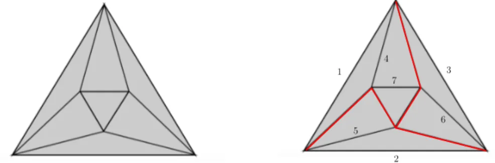
1 2 3 4 5 6 7
Figure 1 The above complex does not have any dominated vertex and thus cannot be 0-collapsed. However, by proceeding from the boundary edges, one can edge collapse this complex to a 1-dimensional complex. The 1-core obtained in this way is collapsible to a point using 0-collapse.
Efficiency of reduction. As will be demonstrated in Section 6, edge collapse appears to be a very efficient tool to reduce the size of a complex while preserving its homotopy type. A simple example will help giving some intuition why edge collapse can be superior to vertex collapse. See Figure 1.
1 2 3 4 5 6 1 2 3 4 5 6 1 2 3 4 5 6
Figure 2 The complex on the left has two different 1-cores, the one in the middle is obtained after removing the inner edges [1, 3] and [4, 6], and the one in the right by removing the outer edges [1, 2] and [4, 5]. Note that the one in the right can be further strong collapsed.
4
Simple Collapse and Persistence
In this section, we turn our attention to the general case of simple collapses (of which k-collapses are a special case) and provide one of the main result of this article. This can be seen as a generalization of Theorem 2 of [12].
ITheorem 4. Let f : K → L be a simplicial map between two complexes K and L and let K0 ⊂ K and L0 ⊂ L be subcomplexes of K and L such that K & K0 and L & L0. Then there exists a map f0: K0 → L0, induced by f , such that the persistence of f∗: H
p(K) → Hp(L)
and f0∗: Hp(K0) → Hp(L0) are the same for any integer p ≥ 0. The induced map f0 may not
be simplicial. Nevertheless, it can be expressed as a combination of inclusions, contractions and removals of simplices.
Proof. Let us consider the following diagram between the geometric realizations of the complex |K|, |L|, |K0| and |L0|. |K| |L| |K0| |L0| |f | |rk| |rl| |f0| |ik| |il|
and the associated diagram after computing the p-th singular homology groups Hpo(|K|) Hpo(|L|) Ho p(|K0|) Hpo(|L0|) |f |∗ |rk|∗ |rl|∗ |f0|∗ |ik|∗ |il|∗
Here |rk| and |rl| are the deformation retractions on the geometric realizations associated
with the simple collapse and |ik| and |il| are the inclusion maps. Hpo() denotes the singular
homology and * is the induced homomorphisms by the corresponding continuous maps. The map |f0| is defined as |f0| := |r
that, since |rk| is a deformation retraction, |ik||rk| is homotopic to the identity over |K|.
It follows that |rl||f ||ik||rk| is homotopic to |rl||f |. Since homotopic maps induce identical
homomorphisms on the corresponding homology groups [38, Proposition 2.19], we deduce that |f0|∗|r
k|∗= |rl|∗|f |∗ (commutativity). Also, since |rk|∗and |rl|∗ are induced by deformation
retractions, they are isomorphisms on their respective singular homology groups. We have thus proved that the above diagram commutes and that the vertical maps |rk| and |rl| are
isomorphisms. This implies that the two maps |f | : |K| → |L| and |f0| : |K0| → |L0| have the same singular persistent homology.
|f0| induces a map f0 := r
l◦ f ◦ ik between the simplicial complexes K0 and L0. Note that
f0 can be expressed as a composition of inclusions, contractions and removals of simplices, as ik is an inclusion, f is simplicial and rl is a simple collapse. Also, for simplicial complexes,
singular homology is isomorphic to simplicial homology [38, Theorem 2.27]. This implies that the persistent singular homology |f0|∗ : Ho
p(|K0|) → H o
p(|L0|) and the persistent simplicial
homology f0∗ : Hp(K0) → Hp(L0) are equivalent. Therefore, the persistent simplicial
homologies f∗: Hp(K) → Hp(L) and f0
∗
: Hp(K0) → Hp(L0) are equivalent. J
The use of singular homology in the proof is due to the lack of a simplicial map associated with the retraction (|r|) of a simple collapse. Due to the same reason, the induced map f0: K0 → L0 may not be necessarily simplicial. However, as mentioned in the above proof the map f0 can be expressed as a combination of inclusions, contractions and removals of simplices. When a sequence of simplicial complexes contains removals of simplices, it is called a zigzag sequence. There are algorithms [45, 42] to compute zigzag persistence but they are not as efficient as the usual algorithms for filtrations and towers.
In the next section, we consider the case of flag filtrations and show that we can restrict the way the edge collapses are performed so that the reduced filtration is also a flag filtration.
5
Edge collapse of a flag filtration
In Section 3, we have introduced edge collapse for general simplicial complexes and provided an easy criterion for edge-domination in a flag complex using only the 1-skeleton of the complex. In this section, we provide an algorithm to simplify a flag filtration by removing dominated edges (i.e. edge collapses), again using only the 1-skeleton of the complex.
We define a notion of removable edge to help explain how our algorithm works (Al-gorithm 1) and to prove its correctness. Let G be a graph and K be the associated flag complex. We say that an edge e in a graph G is removable either if it is dominated in K or if there exists a sequence of edge collapses K&&1Kc such that e is dominated in the
reduced complex Kc. Our algorithm is based on the fact that the flag complexes K and Kc
are homotopy equivalent [53, Lemma 2.7] and [4, Lemma 8]. If e = [u, v], we define the edge-neighborhood of an edge e ∈ G as the set ENG(e) := {[x, y], x ∈ {u, v}, y ∈ NG([uv])}.
Algorithm. Let F : K1 ,→ K2 ,→ · · · ,→ Kn be a flag filtration and GF : G1 ,→ G2 ,→ · · · ,→ Gn be the associated sequence of 1-skeletons. We further assume that Gi ,→ Gi+1 is
an elementary inclusion, namely the inclusion of a single edge we name ei+1. The edges in
E := {e1, ..., en} are thus indexed by their order in the filtration and we denote by Gi the
subset {e1, ..., ei}. Our algorithm computes a subset of edges Ec ⊆ E and attach to each
edge in Ec a new index. We thus obtain a new sequence of flag complexes Fc corresponding
to Ec, we call the core sequence. The construction of Ec and of the new indices is done so that Fc has the same persistence diagram as F .
Let’s give an intuitive presentation of the algorithm first. The central idea is to identify edges that appear to be non-removable at some point in the algorithm. We store such edges
in a set Ec. To be more specific, consider the case of the inclusion of an edge Gi−1 ei
,−→ Gi
such that ei is dominated in Gi : ei is thus removable in Gi and is not included in Ec.
Suppose first that all further edges es are dominated in Gs, i < s ≤ n. Then ei remains
removable and will never be put in Ec. This is consistent with the fact that e
i does not
change the topology of the complexes Ks and is therefore not required when computing
persistence.
Assume now that some edge ep, i < p ≤ n, is non-dominated in Gp. The status of ei,
that was removable in all Gs for s < p, may change to non-removable in Gp. Therefore, we
check whether ei is non-removable in Gp (by proceeding in the reverse filtration order) and,
in the affirmative, include ei in Ec. In turn, the fact that ei changed from removable to
non removable may change the status of the edges with smaller indices which could become non-removable after the inclusion of ei. If such edges are found, they are also included in Ec.
Before describing the algorithm in detail, two remarks are in order. First, we do not change the status of an edge from non-removable to removable even if it has become removable: this will enforce the output sequence to be a filtration. Second, we change the filtration values of some edges: the new filtration value of an edge is the first index at which it is found to be non-removable. The second point leads to faster computation of Ec, otherwise one has to
proceed backward recursively to search for new non-removable edges.
We now explain how to compute Ec. See [Algorithm 1] for the pseudo-code. The main
for loop on line 6 (called the forward loop) iterates over the edges in the filtration F by increasing filtration values, i.e. in the forward direction, and check whether or not the current edge ei is dominated in the graph Gi. If not, we insert ei in Ec and keep its original index i.
After the insertion of an edge eiin Ec, we proceed to the so-called backward loop ([Lines
9-26]) and look for new non-dominated edges in Gi, considering the edges by decreasing
filtration values. We assign Gito a temporary graph G, and we assign the edge-neighborhood
of ei in the graph Gi to Enbd [Line 9-10]. As established in Lemma 5, the search for new
non-dominated edges can be restricted to Enbd. If an edge ej is not in Ec and not in Enbd
[Line 13-14], ej is still dominated : we then remove it from G [Line 22]. If ej 6∈ Ec and
ej∈ Enbd, then we check whether it is dominated or not. If ej is dominated, we remove it
from G [Line 19]. Otherwise, we insert ej in Ec and assign to it the new index i, i.e. the
index of the edge ei that has triggered the backward search in Gi. Next we enlarge the
edge-neighborhood Enbdby inserting the edge-neighbors of ej in G. We repeat this process
until the last index j = 1. Upon termination of the forward loop [Line 6-30], we output Ec
as the final set.
The computation of non-removable edges (the set Ec) is dependent on the order in which
we do the backward search (the backward loop). In Algorithm 1 we chose to proceed in the reverse order of the filtration. A different choice of order might result in a different set of non-removable edges since edge collapses are order dependent as mentioned in Section 3.
We now prove the correctness of the above algorithm after some more definitions.
Critical Edges. Edges in Ecare called critical while edges in E \Ecare called non-critical. All edges have an original index i given by the insertion order in the input filtration F . The critical edges received a second index j, called their critical index, when they are inserted in Ec. By convention, if an edge is not critical and thus has never been inserted in Ec, we
will set its critical index to be ∞. Hence, at the end of Algorithm 1, each edge e ∈ E has two indices, an original and a critical index. To make this explicit, we denote e as eji. Clearly i ≤ j. We further distinguish the cases i = j and i < j. If i = j, ei has been put in Ec
during the forward loop and we call ei a primary critical edge. If i < j, ei has been put
Algorithm 1 Core flag filtration algorithm.
1: procedure Core-Flag-Filtration(E)
2: input : set of edges E of GF sorted by filtration value.
3: Ec← ∅; i ← 1;
4: Enbd← ∅
5: G ← ∅
6: for ei∈ E do . For i = 1, ..., n in increasing order
7: if ei is non-dominated in Gi then 8: Insert {ei, i} in Ec. 9: G ← Gi 10: Enbd← EN Gi(ei) 11: j ← i − 1
12: for ej in Gi do . For j = (i − 1), ..., 1 in decreasing order
13: if ej∈ E/ c then 14: if ej ∈ Enbdthen 15: if ej is non-dominated in G then 16: Insert {ej, i} in Ec. 17: Enbd← Enbd∪ EN G(ej) 18: else 19: G ← G \ ej 20: end if 21: else 22: G ← G \ ej 23: end if 24: end if 25: j ← j − 1 26: end for 27: end if 28: G ← ∅ 29: i ← i + 1 30: end for
31: return Ec . Ec is the 1-skeleton of the core flag filtration.
32: end procedure
For i = 1, ..., n, we define the critical graph at index i, denoted Gci, as the graph whose edges are the edges in Ec with a critical index at most i. We denote the associated flag
complex as Kic.
Correctness. We now prove some lemmas to certify the correctness of our algorithm. The following lemma justifies the fact that the search for new critical edges during the backward loop of Algorithm 1 is restricted to the neighborhood of already found critical edges.
ILemma 5. Let e be an edge in a graph G and let e0 be a new edge and G0:= G ∪ e0. If e is dominated in G and e /∈ ENG0(e0), then e is dominated in G0.
Proof. Let e ≺ v0 in G, then NG[e] ⊆ NG[v0]. Plainly, NG[v0] ⊆ NG0[v0] and, since e /∈
ENG0(e0), NG0[e] = NG[e]. Therefore, NG0[e] = NG[e] ⊆ NG0[v0] implies e ≺ v0 in G0. J
The following lemma says that a non-critical edge is always removable and that a critical edge is removable until it becomes critical.
ILemma 6. Let eji be an edge with i < j, then it is removable in all Gt, i ≤ t < min(n+1, j).
Proof. According to the algorithm, if i < j, eji is dominated in Gi (j being finite or not).
1. Let us first consider the case j = ∞. Note that e∞i is non-critical and let ji be the
smallest primary critical index greater than i. If no such index exists, set ji= n + 1. We
show by induction that e∞i remains removable in all Gt, i ≤ t < n + 1. As shown above, it
is true for t = i since eji is dominated in Gi. So assume that eji is removable in Gt−1and
consider the insertion of etin Gt, for some t < ji. By definition of ji, etis dominated in
Gt, which implies that eji is removable in Gt(in the backward sequence et, et−1, . . . , ei).
Consider now t = ji. Since eji is a primary critical edge, it is non-dominated in Gji.
According to the algorithm, a backward loop has been triggered at ji. During this
backward loop, e∞i has not been inserted in Ec since its second critical index is ∞. This is only possible because e∞i has been found to be dominated in G. Since G is initialized as Gji, it follows that e
∞
i is removable in Gji. We can now proceed in a similar way for
all t, ji< t < n + 1.
2. The proof is very similar for the case i < j ≤ n. As eji has not been inserted in Ec until
the backward loop triggered at index j, eji remains removable in all Gt, i ≤ t < j. J
Note that our statement does not imply that a critical edge eji, i < j ≤ n, can never be removable in Gt, t ≥ j. It just means that we are sure that it will remain removable until
the point it becomes critical.
ILemma 7. For each i, Algorithm 1 produces a sequence of elementary edge collapses such that Ki&&1Kic.
Proof. By definition, Gi\ Gci = {e m
t | t ≤ i, m > i} is the set of edges of Gi whose critical
index m is greater than i, which includes the non-critical edges (m = ∞). Any edge em
t ∈ Gi\ Gci is removable in all Kj, j < m by Lemma 6. J
The proof of the following theorem certifying the correctness of our algorithm follows directly through the application of Lemma 7 and Theorem 4.
ITheorem 8. Let F : K1 ,→ K2 ,→ · · · ,→ Kn be a flag filtration and GF : G1 ,→ G2 ,→ · · · ,→ Gn be the associated sequence of 1-skeletons, such that Gi,→ Gi+1 is an elementary
inclusion of an edge ei+1. Let Gci be the critical graph and Kic be its flag complex as defined
before. Then the associated flag filtration of the critical edges, Fc: Kc
1,→ K2c,→ · · · ,→ Knc
has the same persistence diagram as F .
Proof. Let us consider the following diagram of the geometric realizations of the flag complexes for any i ∈ {1, ..., n}, where Kc
i is the flag complex of the critical graph Gci.
|Ki| |Ki+1|
|Kc
i| |Ki+1c |
|ri| |ri+1|
Using Lemma 7, there is an edge collapse and therefore a simple collapse from Ki to
Kic and from Ki+1 to Ki+1c . And |ri| and |ri+1| are the deformation retractions induced by
the corresponding edge collapses. The equivalence of the persistence modules then follows
Complexity. Write nv for the total number of vertices, n for the total number of edges and
k for the maximum degree of a vertex in Gn. We represent each graph Gi as an adjacency
list, where every vertex stores a sorted list of at most k adjacent vertices. Additionally, we store the set of edges (E and Ec) as a separate data structure.
The cost of inserting and removing an edge from such an adjacency list is O(k). Since the size of NG[v] is at most k for any vertex v, the cost of computing NG[e] for an edge e is
O(k). Checking if an edge e is dominated by a vertex v ∈ NG[e] reduces to checking whether
NG[e] ⊆ NG[v], see Lemma 2. Since all the lists are sorted, this operation takes O(k) time
per vertex v, hence O(k2) time in total.
Let us now analyze the worst-case time complexity of Algorithm 1. At each step i of the forward loop [Line 6], either ei is dominated (which can be checked in O(k2) time) or a
backward loop is triggered [Line 12]. The backward loop will consider all edges with (original) index at most i and check whether they are dominated or not. Writing nc for the number of
primary critical edges, the worst-case time complexity is nk2+Pnc
i=1n k
2= O(nn
ck2). The
space complexity is O(n). In practice, nc is a small fraction of n (see Table 1).
6
Computational Experiments
Our algorithm [Algorithm 1] has been implemented for VR filtrations as a C++ module named EdgeCollapser. Our previous preprocessing method described in [11] to simplify VR filtrations using strong collapses is called VertexCollapser (previously called RipsCollapser). Both EdgeCollapser and VertexCollapser take as input a VR filtration and return the reduced flag filtration according to their respective algorithms.
We present results on five datasets netw-sc, senate, eleg, HIV and torus. The first four datasets are publicly available [22] and are given as the interpoint distance matrix of the points. The last dataset torus has 2000 points sampled in a spiraled fashion on a torus embedded in a 3-sphere of R4[39]. The reported time includes the time of EdgeCollapser/VertexCollapser and the time to compute the persistence diagram (PD) using the Gudhi library [37].
The code has been compiled using the compiler “clang-900.0.38” and all computations were performed on a “2.8 GHz Intel Core i5” machine with 16 GB of available RAM. Both EdgeCollapser and VertexCollapser work irrespective of the dimension of the complexes associated to the input datasets. However, the size of the complexes in the reduced filtration, even if much smaller than in the original filtration, might exceed the capacities of the PD computation algorithm. For this reason, we introduced, as in Ripser [6], a parameter dim and restricts the expansion of the flag complexes to a maximal dimension dim.
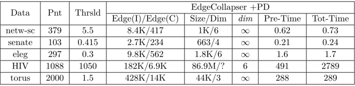
The experimental results using EdgeCollapser are summarized in Table 1. Observe that the reduction in the number of edges done by EdgeCollapser is quite significant. The ratio between the number of initial edges and the number of critical edges is approximately 20. Therefore the reduction in the size of k-simplices can be as large as O(20k). This is
verified experimentally too, as the reduced complexes are small and of low dimension (column Size/Dim) compared to the input VR-complexes which are of dimensions respectively 57, 54 and 105 for the first three datasets netw-sc, senate and eleg.1
Comparison with VertexCollapser. The same set of experimental results using Vertex-Collapser are summarized in Table 2. VertexVertex-Collapser can be used in two modes: in the exact mode (step=0), the output filtration has the same PD as the input filtration while,
in the approximate mode (step>0), a certified approximation is returned. For appropriate comparison, we use VertexCollapser in exact mode. It can be seen that EdgeCollapser is faster than VertexCollapser by approximately two orders of magnitude. The main reason for this is the efficient preprocessing algorithm behind EdgeCollapser. As it can be noticed in some cases, the reduction obtained using VertexCollapser is better than using EdgeCollapser, but even in those cases EdgeCollapser is faster than VertexCollapser.
In terms of size reduction, EdgeCollapser either outperforms VertexCollapser by a big amount or is comparable. Some intuition can be gained from the torus example. This is a well distributed point sets sampled from a manifold without boundary. The fact that there is no boundary implies that there are only a few number of dominated vertices, which dramatically reduces the capacity of VertexCollapser to collapse.
EdgeCollapser computes the exact PD of the input filtration while VertexCollapser has an exact and an approximate modes, Results in Table 2 are obtained using the exact mode of VertexCollapser, while results in Table 1 [11] are obtained using the approximate mode. In both cases, EdgeCollapser performs much better than VertexCollapser. An approximate version of EdgeCollapser can be easily implemented similarly to the case of VertexCollapser. Instead of triggering the backward loop of the algorithm [Line12-26] at each primary critical edge we find, we can trigger the backward loop at certain snapshot values only. See Section 5 of [11] for more details on the approximate methodology and description of snapshot.
Table 1 The columns are, from left to right: dataset (Data), number of points (Pnt), max-imum value of the scale parameter (Thrsld), Initial number of edges/Critical (final) number of edges Edge(I)/Edge(C), number of simplices (Size) and dimension of the final filtration (Dim), parameter (dim), time (in seconds) taken by Edge-Collapser and total time (in seconds) including PD computation (Tot-Time).
Data Pnt Thrsld EdgeCollapser +PD
Edge(I)/Edge(C) Size/Dim dim Pre-Time Tot-Time
netw-sc 379 5.5 8.4K/417 1K/6 ∞ 0.62 0.73
senate 103 0.415 2.7K/234 663/4 ∞ 0.21 0.24
eleg 297 0.3 9.8K/562 1.8K/6 ∞ 1.6 1.7
HIV 1088 1050 182K/6.9K 86.9M/? 6 491 2789
torus 2000 1.5 428K/14K 44K/3 ∞ 288 289
Table 2 The columns are, from left to right: dataset (Data), number of points (Pnt), maximum value of the scale parameter (Thrsld), number of simplices (Size) and dimension of the final filtration (Dim), parameter (dim), time (in seconds) taken by VertexCollapser, total time (in seconds) including PD computation (Tot-Time), parameter Step (linear approximation factor) and the number of snapshots used (Snaps). For the last experiment (torus), the preprocessing was stopped after 12hrs due to the number of snapshots and the size of the complexes.
Data Pnt Thrsld VertexCollapser +PD
Size/Dim dim Pre-Time Tot-Time Step Snaps
netw-sc 379 5.5 175/3 ∞ 366.46 366.56 0 8420
senate 103 0.415 417/4 ∞ 15.96 15.98 0 2728
eleg 297 0.3 835K/16 ∞ 518.36 540.40 0 9850
HIV 1088 1050 127.3M/? 4 660 3,955 4 184
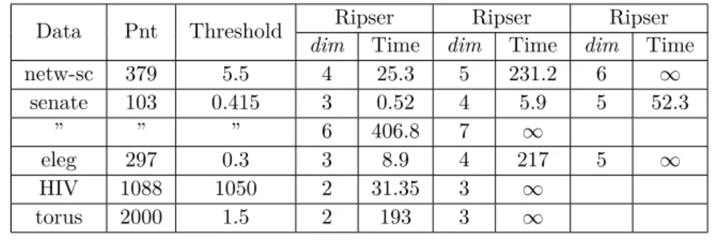
Comparison with Ripser. Ripser is a state-of-the-art software to compute the persistent homology of VR-complexes [6]. Ripser computes the exact PD associated to an input filtration up to some dimension dim. EdgeCollapser (as well as VertexCollapser) are not really competitors of Ripser since they act more as a preprocessing of the input filtration and do not compute Persistence Homology and can be associated to any software computing PH of flag filtrations. Nevertheless, we run Ripser2 on the same datasets as in Table 1 to demonstrate the benefit of using EdgeCollapser. Results are presented in Table 3. The main observation is that, in most of the cases, EdgeCollapser computes PD in all dimensions and outperforms Ripser, even when we restrict the dimension of the input filtration given to Ripser.
Table 3 Time is the total time (in seconds) taken by Ripser. ∞ means that the experiment ran longer than 12 hours or crashed due to memory overload.
Data Pnt Threshold Ripser Ripser Ripser
dim Time dim Time dim Time
netw-sc 379 5.5 4 25.3 5 231.2 6 ∞ senate 103 0.415 3 0.52 4 5.9 5 52.3 ” ” ” 6 406.8 7 ∞ eleg 297 0.3 3 8.9 4 217 5 ∞ HIV 1088 1050 2 31.35 3 ∞ torus 2000 1.5 2 193 3 ∞ References
1 M. Adamaszek and J. Stacho. Complexity of simplicial homology and independence complexes of chordal graphs. Computational Geometry: Theory and Applications, 57:8–18, 2016.
2 D. Attali, A. Lieutier, and D. Salinas. Efficient data structure for representing and simplifying simplicial complexes in high dimensions. International Journal of Computational Geometry
and Applications (IJCGA), 22:279–303, 2012.
3 Dominique Attali and André Lieutier. Geometry-driven collapses for converting a čech complex into a triangulation of a nicely triangulable shape. Discrete & Computational Geometry, 54(4):798–825, 2015.
4 Dominique Attali, André Lieutier, and David Salinas. Vietoris-rips complexes also provide topologically correct reconstructions of sampled shapes. Computational Geometry, 46(4):448– 465, 2013.
5 J. A. Barmak and E. G. Minian. Strong homotopy types, nerves and collapses. Discrete and
Computational Geometry, 47:301–328, 2012.
6 U. Bauer. Ripser. URL: https://github.com/Ripser/ripser.
7 U. Bauer, M. Kerber, and J. Reininghaus. Clear and compress: Computing persistent homology in chunks. In Topological Methods in Data Analysis and Visualization III, Mathematics and
Visualization, pages 103–117. Springer, 2014.
8 U. Bauer, M. Kerber, J. Reininghaus, and H. Wagner. PHAT – persistent homology algorithms toolbox. Journal of Symbolic Computation, 78, 2017.
9 J-D. Boissonnat and C. S. Karthik. An efficient representation for filtrations of simplicial complexes. In ACM Transactions on Algorithms, 2018.
10 J-D. Boissonnat, C. S. Karthik, and S. Tavenas. Building efficient and compact data structures for simplicial complexes. Algorithmica, 79:530–567, 2017.
11 J-D. Boissonnat and S. Pritam. Computing persistent homology of flag complexes via strong collapses. International Symposium on Computational Geometry (SoCG), 2019.
12 J-D. Boissonnat, S.Pritam, and D. Pareek. Strong Collapse for Persistence. In 26th Annual
European Symposium on Algorithms (ESA 2018), volume 112, 2018.
13 M. Botnan and G. Spreemann. Approximating persistent homology in euclidean space through collapses. Applicable Algebra in Engineering, Communication and Computing, 26:73–101, 2015.
14 G. Carlsson and V. de Silva. Zigzag persistence. Found Comput Math, 10, 2010.
15 G. Carlsson, V. de Silva, and D. Morozov. Zigzag persistent homology and real-valued functions.
International Symposium on Computational Geometry (SoCG), pages 247–256, 2009. 16 G. Carlsson, T. Ishkhanov, V. de Silva, and A. Zomorodian. On the local behavior of spaces
of natural images. In: International Journal of Computer Vision, 76:1–12, 2008.
17 J. M. Chan, G. Carlsson, and R. Rabadan. Topology of viral evolution. In: Proceedings of the
National Academy of Sciences, 110:18566–18571, 2013.
18 F. Chazal and S. Oudot. Towards persistence-based reconstruction in Euclidean spaces.
International Symposium on Computational Geometry (SoCG), 2008.
19 C. Chen and M. Kerber. Persistent homology computation with a twist. In European Workshop
on Computational Geometry (EuroCG), pages 197–200, 2011.
20 Aruni Choudhary, Michael Kerber, and Sharath Raghvendra. Polynomial-Sized Topological Approximations Using the Permutahedron. In Sándor Fekete and Anna Lubiw, editors, 32nd
International Symposium on Computational Geometry (SoCG 2016), volume 51 of Leibniz International Proceedings in Informatics (LIPIcs), pages 31:1–31:16, Dagstuhl, Germany, 2016.
Schloss Dagstuhl–Leibniz-Zentrum fuer Informatik. URL: http://drops.dagstuhl.de/opus/ volltexte/2016/5923, doi:10.4230/LIPIcs.SoCG.2016.31.
21 H. Edelsbrunner D. Cohen-Steiner and J. Harer. Stability of persistence diagrams. Discrete
and Compututaional Geometry, 37:103–120, 2007.
22 Datasets. URL: https://github.com/n-otter/PH-roadmap/.
23 V. de Silva and R. Ghrist. Coverage in sensor networks via persistent homology. In: Algebraic
and Geometric Topology, 7:339 – 358, 2007.
24 H. Derksen and J. Weyman. Quiver representations. Notices of the American Mathematical
Society, 52(2):200–206, February 2005.
25 T. K. Dey, H. Edelsbrunner, S. Guha, and D. Nekhayev. Topology preserving edge contraction.
Publications de l’Institut Mathematique (Beograd), 60:23–45, 1999.
26 T. K. Dey, F. Fan, and Y. Wang. Computing topological persistence for simplicial maps. In
International Symposium on Computational Geometry (SoCG), pages 345–354, 2014. 27 T. K. Dey, D. Shi, and Y. Wang. SimBa: An efficient tool for approximating Rips-filtration
persistence via Simplicial Batch-collapse. In European Symp. on Algorithms (ESA), pages
35:1–35:16, 2016.
28 T. K. Dey and R. Slechta. Filtration simplification for persistent homology via edge contraction.
International Conference on Discrete Geometry for Computer Imagery, 2019.
29 C. H. Dowker. Homology groups of relations. The Annals of Mathematics, 56:84–95, 1952.
30 P. Dłotko and H. Wagner. Simplification of complexes for persistent homology computations,.
Homology, Homotopy and Applications, 16:49–63, 2014.
31 H. Edelsbrunner and J. Harer. Computational Topology: An Introduction. American Mathem-atical Society, 2010.
32 H. Edelsbrunner, D. Letscher, and A. Zomorodian. Topological persistence and simplification.
Discrete and Compututational Geometry, 28:511–533, 2002.
33 Omer Egecioglu and Teofilo F. Gonzalez. A computationally intractable problem on simplicial complexes. Computational Geometry, 6:85–98, 1996.
34 B. T. Fasy, J. Kim, F. Lecci, and C. Maria:. Introduction to the R-package tda. CoRR
35 E. Fieux and J. Lacaze. Foldings in graphs and relations with simplicial complexes and posets.
Discrete Mathematics, 312(17):2639–2651, 2012.
36 F. Le Gall. Powers of tensors and fast matrix multiplication. ISSAC ’, 14:296–303, 2014.
37 Gudhi: Geometry understanding in higher dimensions. URL: http://gudhi.gforge.inria. fr/.
38 A. Hatcher. Algebraic Topology. Univ. Press Cambridge, 2001.
39 Benoît Hudson, Gary L. Miller, Steve Oudot, and Donald R. Sheehy. Topological inference via meshing. International Symposium on Computational Geometry (SoCG), 2010.
40 M. Kerber and H. Schreiber:. Barcodes of towers and a streaming algorithm for persistent homology. International Symposium on Computational Geometry (SoCG), 2017. arXiv: 1701.02208.
41 M. Kerber and R. Sharathkumar. Approximate Čech complex in low and high dimensions. In
Algorithms and Computation, pages 666–676. by Leizhen Cai, Siu-Wing Cheng, and Tak-Wah
Lam. Vol. 8283. Lecture Notes in Computer Science, 2013.
42 C. Maria and S. Oudot. Zigzag persistence via reflections and transpositions. In Proc.
ACM-SIAM Symposium on Discrete Algorithms (SODA) pp. 181–199, January 2015. 43 N. Milosavljevic, D. Morozov, and P. Skraba. Zigzag persistent homology in matrix
multiplic-ation time. In Internmultiplic-ational Symposium on Computmultiplic-ational Geometry (SoCG), 2011.
44 K. Mischaikow and V. Nanda. Morse theory for filtrations and efficient computation of persistent homology. Discrete and Computational Geometry, 50:330–353, September 2013.
45 D. Mozozov. Dionysus. URL: http://www.mrzv.org/software/dionysus/.
46 J. Munkres. Elements of Algebraic Topology. Perseus Publishing, 1984.
47 N. Otter, M. Porter, U. Tillmann, P. Grindrod, and H. Harrington. A roadmap for the computation of persistent homology. EPJ Data Science, Springer Nature, page 6:17, 2017.
48 Steve Y. Oudot and Donald R. Sheehy. Zigzag zoology: Rips zigzags for homology inference.
Foundations of Computational Mathematics, 15, 2015.
49 J. Perea and G. Carlsson. A Klein-bottle-based dictionary for texture representation. In:
International Journal of Computer Vision, 107:75–97, 2014.
50 H. Schreiber. Sophia. URL: https://bitbucket.org/schreiberh/sophia/.
51 D. Sheehy. Linear-size approximations to the Vietoris–Rips filtration. Discrete and
Computa-tional Geometry, 49:778–796, 2013.
52 M. Tancer. Recognition of collapsible complexes is NP-complete. Discrete and Computational
Geometry, 55:21–38, 2016.
53 Volkmar Welker. Constructions preserving evasiveness and collapsibility. Discrete Mathematics, 207(1):243–255, 1999.
54 J. H. C Whitehead. Simplicial spaces nuclei and m-groups. Proc. London Math. Soc, 45:243–327, 1939.
55 A. C. Wilkerson, H. Chintakunta, and H. Krim. Computing persistent features in big data: A distributed dimension reduction approach. In International Conference on Acoustics, Speech,
and Signal Processing (ICASSP), pages 11–15, 2014.
56 A. C. Wilkerson, T. J. Moore, A. Swami, and A. H. Krim. Simplifying the homology of networks via strong collapses. In International Conference on Acoustics, Speech, and Signal
Processing (ICASSP), pages 11–15, 2013.
57 A. Zomorodian. The tidy set: A minimal simplicial set for computing homology of clique complexes. In International Symposium on Computational Geometry (SoCG), pages 257–266, 2010.
58 A. Zomorodian and G. Carlsson. Computing persistent homology. Discrete and Computational
![Figure 2 The complex on the left has two different 1-cores, the one in the middle is obtained after removing the inner edges [1, 3] and [4, 6], and the one in the right by removing the outer edges [1, 2] and [4, 5]](https://thumb-eu.123doks.com/thumbv2/123doknet/13315015.399199/7.892.192.721.243.395/figure-complex-different-cores-middle-obtained-removing-removing.webp)