HAL Id: halshs-01159507
https://halshs.archives-ouvertes.fr/halshs-01159507v2
Submitted on 3 May 2016
HAL is a multi-disciplinary open access archive for the deposit and dissemination of sci-entific research documents, whether they are pub-lished or not. The documents may come from teaching and research institutions in France or abroad, or from public or private research centers.
L’archive ouverte pluridisciplinaire HAL, est destinée au dépôt et à la diffusion de documents scientifiques de niveau recherche, publiés ou non, émanant des établissements d’enseignement et de recherche français ou étrangers, des laboratoires publics ou privés.
Welfare Analysis of the Allocation of Time During the
Great Recession
Anil Alpman, François Gardes
To cite this version:
Anil Alpman, François Gardes. Welfare Analysis of the Allocation of Time During the Great Recession. 2016. �halshs-01159507v2�
Documents de Travail du
Centre d’Economie de la Sorbonne
Welfare Analysis of the Allocation of Time During
the Great Recession
Anil A
LPMAN,François
G
ARDESWelfare Analysis of the Allocation of Time During the
Great Recession
Anil Alpman and Fran¸cois Gardes⇤
March 19, 2016
Abstract
Using a generalization of the time allocation model to estimate the op-portunity cost of time, we explore the intratemporal substitutions between goods and time and the variations of individuals’ full expenditures and wel-fares during the Great Recession. Our findings provide empirical evidence about the importance the home production over the business cycles and show that the reallocation of time absorbed approximately a third of the Great Recession’s negative welfare impact.
Keywords: Home Production, Time Allocation, Welfare, Great Re-cession.
JEL: D31, J22.
⇤Alpman and Gardes: Paris School of Economics and Universit´e Paris 1 Panth´eon-Sorbonne,
106 - 112 Boulevard de l’Hˆopital, 75013 Paris, anil.alpman@gmail.com, francois.gardes@univ-paris1.fr.
We would like to thank the participants at the congresses of the ‘European Economic Associ-ation’, the ‘Soci´et´e Canadienne de Science Economique’, the ‘Association Fran¸caise de Science Economique’ and the ‘Journ´ees de Micro´economie Appliqu´ee’ for their helpful remarks.
1
Introduction
Looking only to the variations of individuals’ monetary incomes would yield an incomplete picture of individuals’ welfare losses during the Great Recession be-cause the time freed-up by unemployment or underemployment may be used in activities such as home production or leisure to compensate partially the loss of income. As Aguiar and Hurst (2007a) note, as soon as non-market work time has value, welfare calculations “based solely on changing incomes or changing expenditures” would be inaccurate. The exclusion of the value of non-market activities has been raised as a serious issue since the introduction of the time al-location model (sometimes referred to as the home production model) by Becker (1965). Indeed, the size of the home sector is quite large (home production equals two-thirds of a household’s total money income on average according to Gronau [1980]) and the extended income, which includes the value of home production, is more equally distributed than the monetary income (see for instance Frick et al. [2012], Frazis and Stewart [2011], and Bonke [1992]).
While these findings provide important insights regarding the welfare im-plications of the home sector, they do not answer an essential question that we address in this paper: during recessions, how much of the welfare loss induced by lower income and lower market work hours are compensated by the increase of the time allocated to home production? A naive analysis of time allocation would be misleading to compute accurately the welfare implications of the Great Re-cession for two reasons. First, common low frequency trends in time use must be controlled for. Aguiar et al. (2013), who obtain their results using the variation of changes in time use across States, show for instance that one would wrongly conclude that leisure absorbs 80% (rather than 50%) of the decline in market work hours during the recession if the trend of leisure time is not controlled for. Second, it is necessary to provide a precise description of the evolution of the substitution between time and monetary ressources over the business cycle, and of its consequences on the value of time and on the consumers’ well-being. We believe that no satisfying answers have been yet proposed regarding the second
point because datasets including time and income allocations are rarely available and therefore little e↵orts have been put to translate the theoretical model of home production into an empirical analysis of the substitutions between time and goods.
We explore in this paper the evolution of individuals’ welfares over 2004 and 2012 in the United States: first, we estimate the value of non-market work time that allows us to quantify the value of the time freed-up during the recession in addition to the monetary income.1 Then, we investigate the relation between the value of time and the intratemporal substitution between time and mone-tary expenditures. Ultimately, we measure the consequences of the substitution between time and monetary expenditures on individuals’ well-being.
To compute the welfare implications of the Great Recession, we use a house-hold production model where the consumer combines time with market goods to produce activities that generate satisfaction. Utility maximization implies that the value of time is given by the ratio of the marginal utility of time over the marginal utility of market goods. A method proposed by Gardes (2014) shows that this ratio can be estimated provided that data on time and income are available. To overcome the lack of this type of data, we use an original statis-tical matching procedure proposed by Rubin (1986) to combine the American Time Use Survey (as processed by Aguiar et al. [2013]) with the Consumer Ex-penditure survey. Unlike Rubin’s procedure, other statistical matching methods assume implicitly that the variables to be matched are conditionally independent, which is a strong assumption that leads to severe biases when this assumption is not verified.
Besides its welfare implications, the value of time plays an important role in real business cycles that should not be neglected: our findings suggest that it is the decrease of the opportunity cost of time, not the real wage rate, that may explain why Aguiar et al. (2013) find out that only 10% of the decline in the market work hours during the Great Recession were allocated to job
1We use a new method (Gardes, 2014) to estimate the value of time which does not require to
assume that the value of an individual’s time is equal to her wage rate or to the housekeeper wage.
search and other income generating activities while 50% of the forgone market work hours were compensated by an increase in leisure and 30% by an increase in non-market work. In other words, our results also provide evidence that the intratemporal substitution between goods and time, induced by changes in relative prices, introduces “a powerful amplification channel to hours worked in response to changes in market productivity” (Aguiar et al., 2013).
Section 2 presents the model that we use to obtain our results. Section 3 describes the dataset and the matching procedure. In Section 4 we present our results and in Section 5 we discuss the implications of our results.
2
The Model
Following Gardes (2014), we assume that the consumer combines time with mon-etary expenditures to produce activities that generate utility in a model where the market work time is valued by the consumer’s wage rate, denoted w, whereas time allocated to other activities (e.g., leisure or non-market work) is valued by the shadow price of time, denoted !.
It is assumed that the consumer’s utility is given by u(Q) =QiaiQii where
ai is a positive parameter and Qi is the activity i produced by the combination
of monetary (m) and time (t) inputs: Qi = bim↵iitii where mi = xipi with xi
the quantity of the market good i, pi its price, and bi a positive parameter. A
Cobb-Douglas structure is assumed both for the utility and for the production functions in order to simplify the derivation of the optimization program. The parameters are estimated locally (i.e., for each observation in the dataset; see the appendix), so that this specification assumes simply constant substitution between time and monetary ressources in the neighborhood of each individual’s equilibrium point.
in terms of inputs: u(m, t) =Y i Ai Y i m ↵i i P ↵i i i !P ↵i i Y i t i i P i i i !P i i (1) = A m0P↵ i t0P i i (2)
where m0 and t0 are geometric weighted means of the monetary and time inputs. Suppose that w di↵ers from the shadow price of time !. In that case, the full expenditure writes:
n
X
i
(pixi+ !ti) = wT + (! w)(T tw) + V (3)
where tw is time allocated to market work, T =Pti+ tw is total time and V is
non-market income less savings. The optimization program consist in maximiz-ing equation (2) subject to equation (3). Note that T tw =Piti and that both
the market wage and ! appear in the budget equation: as mentioned the shadow price of time corresponds to the valuation of the total disposable time when not working on the market and it di↵ers from the market wage w whenever there exists some imperfections, transaction costs, constraints on the labor market or in the domestic production, or when the disutility of labor is smaller for home production.
Denoting the monetary income by Y = wtw+ V , the shadow price of time is
given by ! = @u @t0@t 0 @T @u @m0@m 0 @Y = m 0P i i@t@T0 t0P↵i i@m0 @Y (4) See the Appendix for the derivation of the parameters of the utility and produc-tion funcproduc-tions.
3
The Dataset
The model is estimated on a dataset obtained by matching the American Time Use Survey (ATUS), as it was processed by Aguiar et al. (2013), with the
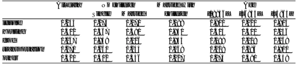
Con-Table 1: Descriptive Statistics ti !ti mi Pti iti mi P imi !ti+ mi !ti+mi yf leisure 29.412 224.754 179.079 0.350 0.161 406.480 0.236 housing 12.579 104.351 253.231 0.145 0.254 364.973 0.207 food 13.705 114.821 107.577 0.171 0.122 224.089 0.136 transport 9.691 73.735 271.604 0.125 0.219 348.475 0.183 other 17.335 140.432 270.292 0.208 0.243 420.167 0.238
Notes: tiand midenote time and monetary income allocated to activity i, respectively; ! denotes
the estimated opportunity cost of time; and yf =P
i(!ti+ mi) denotes the full expenditure.
sumer Expenditure (CE) survey.2 In the CE survey, we use the FMLI file which
contains households’ characteristics, income and summary level expenditures. Given that the ATUS informs the weekly time allocation of one individual within the household, we transform households’ quarterly expenditures into weekly per capita expenditures using the equivalence scale proposed by the OECD that con-sists in dividing expenditures by the square root of the family size. We also divide expenditures by the price index to obtain real expenditures and drop all indi-viduals above 65 and below 18 as in Aguiar et al. (2013). Since the estimation of the shadow price of time requires prior estimates of the production functions’ parameters, we define five activities for which the monetary and time inputs can be accurately identified: leisure, housing (including home work), transport, food and others.
We then match the ATUS and the CE survey using the statistical matching procedure proposed by Rubin (1986). Rubin’s procedure allows to overcome a se-rious issue encountered in other statistical matching procedures: usual matching procedures assume implicitly that the variables to be matched are conditionally independent, that is, if the ATUS and the CE survey were matched using a usual matching procedure, the same amount of expenditures on acitivity i would be imputed to the observations sharing the same demographic characteristics but with di↵erent amounts of time allocated to that activity i. Yet, the time allo-cation literature points out that the income allocated to acitivity i often di↵ers with the amount of time allocated to that activity, everything else equal.
2for a detailed description of both datasets and the matching procedure, see our technical
Table 2: Ratio of the Value of the Time Input Over the Value of Market Goods: !ti/mi.
All data No children Married with Age
Single Married children [18; 36[ [36; 55[ [55; 65]
leisure 1.255 1.273 1.071 1.188 0.901 1.120 0.805
housing 0.412 0.367 0.390 0.940 0.415 0.401 1.036
food 1.067 0.949 1.016 0.934 1.088 1.018 1.068
transportation 0.271 0.261 0.244 1.068 0.229 0.286 0.800
other 0.520 0.412 0.336 1.227 0.274 0.490 0.559
Unlike usual matching procedures, Rubin’s method allows to predict expen-ditures on activity i as a function of the demographic characteristics and the time allocated to that activity (even if expenditures and time allocations are never jointly observed for any unit in the dataset) by assuming a partial corre-lation value between expenditures and time allocated to activity i. Then, the observations of the CE survey are matched with those of the ATUS according to their predicted values (using a minimum distance criterion) conditional on a set of control variables, and the observed value of the match is imputed for the missing.
A Monte Carlo simulation (Alpman, 2015) shows that Rubin’s procedure, compared to usual matching methods, recovers more accurately the distribution of the variables with missing values and it yields consistent inferences when the partial correlation value is assumed correctly. Based on estimates made on Canadian and French data (Gardes, 2014), we match the CE survey and the ATUS assuming a partial correlation value of 0.2 (see the technical appendix for a detailed description regarding the choice of the partial correlation value) between expenditures and time allocated to activity i given the control variables (i.e., state, region, education, age, martial status, number of child, sex and race). The technical appendix o↵ers a detailed descritption of the matching procedure and shows various descriptive statistics.
The first column of Table 1 shows that 82.7 hours per week are allocated to the five activities (leisure, housing, food, transport, and other) while the average market work time and the average sleeping time are equal to 27.5 and 57.7 hours
per week, respectively.3 Among the time spent on these five activites, most of it (i.e., 35%) are allocated to leisure as shown by the fourth column of Table 1. On the other hand, the fifth column of Table 1 shows that most of the monetary income (25.4%) is allocated to housing. The last column of Table 1 shows the full budget share of each activity, that is, the ratio of the full expenditure on activity i over the sum of the full expenditures. Table 1 indicates that looking only to the time shares (column 4) or to the budget shares (column 5) would yield only a partial view regarding the ressources allocated to the activities. Table 2 shows the ratio of the value of the time input (!ti) over the value of market goods (mi)
for each activity. For instance, leisure and food are activites in which the value of market goods are relatively lower than the value of the time input.
4
Results
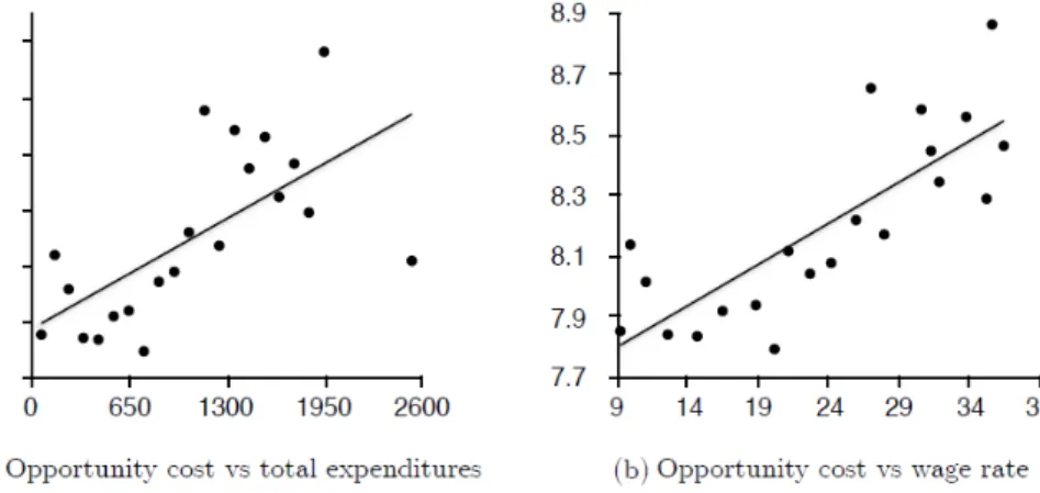
The results indicate (Table 3) that the shadow price of time is 8.10$ on average, that is, 54% of the real wage rate.4 In Figure 1, observations were grouped ac-cording to 21 total expenditures (i.e.,Pimi) categories. The first group includes
observations for which Pimi < 100$ per week. The second group includes
ob-servations for which Pimi 2 [100; 200[ . The third group includes observations
for whichPimi 2 [200; 300[ , and so forth. The last group includes observations
for which Pimi 2, 000$ per week. Graph (a) in Figure 1 shows a positive
relation between the shadow price of time and total expenditures. In line with the economic theory, Graph (b) shows a positive relation between the real wage rate and the shadow price of time. The size of the estimated shadow price of time as well as its relation with the real wage rate suggest that the shadow price of time is estimated accurately.
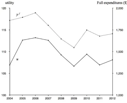
Figure 2 shows that the evolution of the shadow price of time follows the
3The di↵erences between our results and those of Aguiar et al. (2013) are explained by two
factors: the inclusion of the years 2011 and 2012, and a di↵erent definition of the time use categories. When these two factors are taken into account, a comparison shows that the results are quite similar.
4The analysis of the substitution between time and money conducted by Aguiar and Hurst
(2007b) allows to derive a shadow price of time which is quite low (39% of the minimum wage rate) and significantly lower than our estimates (see the technical appendix).
economic cycle as predicted by the time allocation theory: during the period of sustained growth (2004-2006), the shadow price of time has an increasing trend and its average value over this period is equal to 9.43$. As the economic activity slows down significantly in 2007, the shadow price of time decreases by 19.4%. It continues to decrease by 15.6% between 2007 and 2008 and reaches its lowest value during the Great Recession in 2009 (i.e., 6.05$). Over the recovery period (2010-2012), the values of the shadow price of time and of the GDP per capita growth are higher than their crisis values but lower than their values during the sustained growth period: the shadow price of time fluctuates around 7.95$ between 2010 and 2012.
[Insert Table 3 around here]
Since the labor market becomes more attractive for the consumer during growth periods (because of higher wage rates and the higher probability of find-ing a job), in theory the shadow price of time should increase together with the time allocated to market work. Thus, the time input is expected to be substi-tuted by market goods in the production of activities. Figure 1 shows that our results match the theory: during the period of sustained growth (2004-2006), the geometric weighted mean of expenditures (i.e., m0) increases roughly by 11% and reaches its peak in 2006 while the geometric weighted mean of time inputs (i.e., t0) reaches the same year its lowest value (during the same period, the mar-ket work time also increases according to Aguiar et al. [2013]). Between 2007
and 2009, m0 decreases roughly by 9% per year whereas t0 increases by 2% and reaches its highest value in 2009. During the recovery period, m0 and t0 oscillate around lower and higher trends, respectively, than their pre-crisis trends.
The results of Aguiar et al. (2013) indicate that when the market work time decreases by 1%, time allocated to various activities increases by 0.23% on aver-age.5 The substitution between monetary and time inputs, on the other hand,
can be estimated by the elasticity of substitution defined as
= @ log(t0/m0)/@ log(!). Our results show that is 0.37 on average (Hamer-mesh [2008] obtains comparable values). Note that includes implicitely, through the variation of t0, the substitution between market work time and time allocated to other activities; in addition, contains an income e↵ect (through the changes of the market work time and the shadow price of time). Thus, along with the elasticities computed by Aguiar et al. (2013), the value of is an additional result that should be accounted for in the analysis of home production over the business cycle.
Figure 2: The shadow price of time (!) and the geometric weighted means of monetary (m0) and time (t0) inputs.
5Using the share of time allocated to each activity (Aguiar et al. (2013), Table 3, column 1) and
the elasticity of time substitution between each activity and the market work time (denoted ei) computed by Aguiar et al. (2013), we calculate the average elasticity of time substitution
Another important indicator that captures the relations between the mon-etary and the temporal components is the full expenditure (see equation [3]), 63% of which is constituted by monetary expenditures on average. Figure 2 shows that during the sustained growth period, the full expenditure increases by 4.7%; this increase is mainly driven by higher quantities of market goods since expenditures are in real terms. However, the full expenditure decreases by 7.42% between 2006 and 2007, 8.66% between 2007 and 2008, and it reaches its lowest value (1, 546.25$) during the Great Recession after decreasing by 6.11% between 2008 and 2009. During the recovery period, the full expenditure increases by 13.11% but remains under its pre-crisis values. Note that all these changes are greater than those of the growth rate of the per capita GDP.
The evolutions between 2006 and 2009 of the components of the full expen-diture show that the monetary and the time expenexpen-ditures have decreased by 10.28% (i.e., 120.64$) and 36.27% (i.e., 280.52$), respectively, while the time allocated to various activities (i.e., Pti) has increased by 1.93%. According to
these results, the decrease of the monetary expenditures during the Great Re-cession is induced by lower quantities of market goods whereas the decrease of the value of time expenditure is induced by the decrease of the shadow price
of time, which leads to an increase of the time allocated to various non-market activities. Indeed, the elasticity of t0 with respect to the shadow price of time (when the market work time and individual characteristics are controlled for) is 0.08 between 2004 and 2006, 0.14 between 2007 and 2009, and 0.12 between 2010 and 2012. In addition to the forgone market work hours, the decrease of the shadow price of time is therefore an important factor explaining the increase of the time allocated to various activities during the Great Recession. (Note that our estimations indicate that the elasticity of t0 with respect to the market work time is 0.28, which is quite similar to the average weighted elasticity, 0.23, computed using the elasticities informed in Aguiar et al. [2013]).
The decrease of the cost of time and the possibility to substitute time to market goods when the market work time decreases should imply that the evo-lution of the time component during the Great Recession reduces the negative impact of the crisis on individuals’ welfares. The latter is explored by estimating the indirect utility, which is a function of time and expenditures (see equation [2]). Note that the evolution of the utility over the business (see Figure 3) is very much as expected on average: during the period of sustained growth (2004-2006), utility increases while it decreases slightly as the economic activity slows down in 2007. When the growth rate of the GDP per capita becomes negative in 2008, the utility decreases significantly. During the Great Recession, the utility con-tinues to decrease ( 2.4% between 2008 and 2009) and it reaches its lowest value (which is slightly below its 2004 level). Within the recovery period (2010-2012) the utility fluctuates at a higher level than during the crisis but it remains lower to its pre-crisis level. We find out that the elasticities of the utility with respect to m0 and t0 are 0.64 and 0.44, respectively. Finally, if t0 was fixed at its 2006 value, the decrease rate of the utility would have been 35% stronger. Therefore, the time component attenuates indeed the negative impact of the crisis.
5
Discussion
Table 4 shows the results as a function of various demographic characteristics (age, marital status, presence of children, and education level). According to Table 4, monetary expenditures have decreased on average less than 1% between the period of sustained growth and the Great Recession; they have even increased for individuals that are married, young and who have a low education level (this may be explained by the increasing real wage rate during the Great Recession as indicated by our dataset and the findings of Jenkins et al. [2013]). Therefore, welfare calculations based solely on monetary expenditures would yield incorrect conclusions.
Better results can be obtained by looking to the geometric weighted mean of expenditures (i.e., m0), which takes into account the parameters of the pro-duction and the utility functions. However, m0 and total expenditures exclude the use of time and its value. On the other hand, exploring the variations of the full expenditure, which includes monetary expenditures and the value of the time input, overestimates the Great Recession’s welfare impact according to our results since its variations are much greater than any other variables in Table 4, except the shadow price of time. The strong decrease of the full expenditure is explained mainly by the even stronger decrease of the shadow price of time. Yet, a lower shadow price of time implies that the time input becomes relatively cheaper inducing thereby a substitution e↵ect that changes the amounts of the monetary and the time inputs in the production functions. Therefore, this sub-stitution e↵ect reduced the decrease in utility during the recession according to our results. Note that the utility decreased much less than the full-expenditure. In addition, the impact of the crisis explored through the variations in utility give results that are more in line with the findings in the literature: for instance, Table 4 shows that individuals with lower education levels were more a↵ected by the Great Recession in terms of utility than those with higher levels of education as in Jenkins et al. (2013).
behavior, the shadow price of time appears to be a powerful amplifier of business cycles:6 when a recession occurs, the labor demand curve shifts to the left and the downward pressures on the wage rate and the shadow price of time lead market goods to be substituted by the individual’s time as indicated by the value of , which is equal to 0.37. The decrease of monetary expenditures implies a lower aggregate product (measured by monetary indicators). Overall, the substitution between non-market work time and market work hours magnifies the decrease of the market activity
6
Conclusion
This paper provides empirical evidence that changes in the shadow price of time induce an intratemporal substitution between time and market goods that at-tenuates the negative impact of the crisis. According to our estimates, when the decrease rate of the consumption of market goods is equal to the increase rate of the time allocated to non-market activities, the time component absorbs roughly 68.75% of the recession’s negative impact on the consumers’ well-beings. Between 2006 and 2009, m0 has decreased by 12.48% (inducing a 7.99% decrease in welfare) whereas t0 has increased by 5.44% on average (which led to a 2.41% increase in consumers’ welfares). As a consequence, the overall e↵ect has been a 5.58% loss in welfare on average. These results suggest that the time component has absorbed 30% of the Great Recession’s negative welfare impact.
Furthermore, the decrease of the shadow price of time induces a higher volatil-ity in the labor supply: the empirical elasticvolatil-ity of t0 with respect to the market work time is 0.28 according to our results.7 Adding the shadow price of time into the regression of t0 over tw shows that the empirical elasticity of t0 with
re-spect to the shadow price of time is 0.14 between 2007 and 2009 (the coefficient of the market work time remains roughly similar when the shadow price of time is added to the regression). According to these results, 48% of the increase of
6Table 4 shows that the decrease rate of ! is larger than the decrease of monetary expenditures. 7This elasticity is similar to the average weighted elasticity (i.e., 0.23) that was computed, as
the time allocated to non-market activities would be explained by the decrease of the shadow price of time and 52% by the forgone market work hours.
In this paper we were able to compute a shadow price of time at the individual level by relaxing the assumption that the shadow price of time is necessarily equal to individuals’ market wage rates. Estimating the value of time, which is approximately one half of the individuals’ wage rate8, allows to measure the
monetary value of their home production. As Gronau (1980), we find that the value of the time allocated to home production divided by the monetary income is 66.87% when the terms of the ratio are at their sample means. The results that we obtain are thus quite supportive of the procedure used in this paper. Such a procedure could be used to measure and aggregate individuals’ full incomes (i.e., the monetary income plus the value of non-market work time) to compute an enlarged GDP.
Appendix
Following Gardes (2014), the substitution between time and money in the pro-duction function of activity i generates the following first order conditions:
↵i= mi !ti+ mi and i= !ti !ti+ mi (A.1)
under the constraint of a constant economy of scale for each production function, that is, ↵i+ i= 1.
Consider now the substitution between times ti and tj in the production
functions of two di↵erent activities i and j: this substitution implies another condition between the parameters of the utility and the production functions:
i j = jti itj = ajmi aimj (A.2)
All other substitutions between monetary and time ressources devoted to di↵er-ent activities can be derived from equations (A1) and (A2).
Equation (A2) implies for all activities:
mi j= mj i+ ! itj ! jti (A.3)
Equation (A3) can be estimated as a system of (n 1) equations for j = 1 and i = 2, 3, . . . , n under the constraint of P i = 1 or fixing j as the full budget
share of one of the activities, for instance food. In this system, ! and j are
over-identified. Using the shadow price of time estimated from equation (A3), we obtain the estimates of ↵i and ifrom equation (A1) for each individual that
allow to derive estimates of the shadow price of time at the individual level by equation (4).
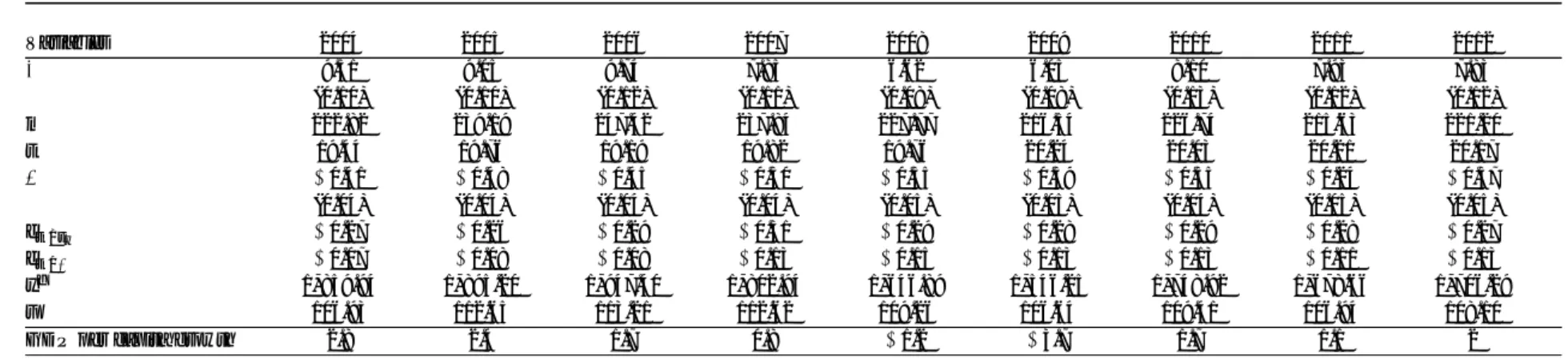
Table 3: Estimations of the Home Production Model Variables 2004 2005 2006 2007 2008 2009 2010 2011 2012 ! 9.51 9.05 9.74 7.85 6.62 6.05 8.10 7.93 7.83 (0.10) (0.10) (0.12) (0.11) (0.08) (0.08) (0.13) (0.12) (0.12) m0 222.82 239.19 247.42 237.84 227.77 216.54 226.74 215.63 221.20 t0 19.44 19.76 19.19 19.82 19.76 20.24 20.03 20.21 20.17 0.41 0.48 0.45 0.30 0.35 0.39 0.35 0.24 0.37 (0.04) (0.04) (0.04) (0.04) (0.05) (0.05) (0.04) (0.05) (0.05) et0/tw 0.27 0.26 0.29 0.31 0.29 0.28 0.29 0.28 0.27 et0/! 0.07 0.08 0.08 0.13 0.15 0.13 0.13 0.11 0.13 yf 1, 859.94 1, 895.20 1, 947.40 1, 802.94 1, 646.89 1, 546.25 1, 748.92 1, 678.66 1, 706.29 u 106.93 112.65 113.21 112.62 109.26 106.64 109.41 106.94 108.10
GDP per capita growth 2.8 2.4 1.7 0.8 1.2 3.7 1.7 1.1 2
Notes: ! is the average shadow price of time for the whole population and the standard error of this mean multiplied by 102is in parentheses; m0and t0are the geometric
weighted means of monetary and time inputs, respectively; = @log(t0/m0)/@log(!) is the elasticity of substitution between time and expenditures with its standard error
in parentheses; et0/tw and et0/!are the elasticities of t0 with respect to the market work time and the shadow price of time, respectively; y
f is the full expenditure; and u
is the utility. All the variables have been estimated at the individual level and averaged over the population.
Table 4: Main Results According to Demographic Characteristics
2004/06 2007 2008/09 2010/12 (c) (a)(a) ⇤ 100
(a) (b) (c) (d)
shadow price of time (!)
Complete dataset 9.42 7.85 6.34 7.95 32.71
singles 9.74 8.60 6.41 8.29 34.22
married with no children 9.88 7.97 6.74 8.33 31.82
married with children 9.10 7.49 6.09 7.62 33.04
age: below 36 9.18 8.17 6.06 7.73 34.00
age: between 36 and 55 9.32 7.63 6.30 7.88 32.45
age: between 56 and 65 10.09 7.96 6.85 8.40 -32.09
education level 1 9.03 7.29 6.20 7.57 31.29
education level 2 9.69 8.29 6.26 8.24 35.41
education level 3 9.58 8.03 6.52 8.07 31.90
Geometric weighted mean of monetary expenditures (m0)
Complete dataset 236.11 237.84 222.14 221.18 5.92
singles 250.02 241.00 232.16 230.69 7.14
married with no children 287.31 289.29 266.09 271.30 7.38
married with children 211.18 211.81 199.50 196.92 5.53
age: below 36 194.69 201.93 184.86 184.54 5.05
age: between 36 and 55 239.45 235.24 224.89 214.91 6.08
age: between 56 and 65 292.99 296.32 268.06 281.28 8.51
education level 1 179.64 188.20 165.18 168.05 8.05
education level 2 241.95 241.74 222.56 214.50 8.01
education level 3 284.86 285.76 272.76 269.04 4.25
Geometric weighted mean of activity times (t0)
Complete dataset 19.48 19.82 20.00 20.14 2.70
singles 18.69 18.66 19.40 19.71 3.79
married with no children 20.21 20.69 20.83 20.88 3.04
married with children 19.78 20.24 20.05 20.25 1.38
age: below 36 18.71 19.13 19.31 19.34 3.20
age: between 36 and 55 19.14 19.30 19.54 19.626 2.09
age: between 56 and 65 21.70 22.20 22.27 22.32 2.61
education level 1 18.74 19.47 19.21 19.51 2.49
education level 2 19.64 20.07 20.47 19.95 4.23
education level 3 20.04 19.97 20.35 20.78 1.54
(Continues from previous page)
Monetary Expenditures
Complete dataset 647.95 632.72 645.42 619.27 0.39
singles 614.51 584.07 580.96 568.77 5.46
married with no children 723.65 700.12 727.49 713.02 0.53
married with children 682.08 665.18 692.14 636.35 1.47
age: below 36 518.55 533.27 523.76 519.30 1.00
age: between 36 and 55 713.13 672.93 704.44 657.58 1.22
age: between 56 and 65 693.98 702.99 690.24 681.38 0.54
education level 1 484.12 492.17 498.16 479.78 2.90 education level 2 561.94 556.12 532.57 550.33 5.23 education level 3 874.08 850.89 848.15 773.48 2.97 Full Expenditure Complete dataset 1,899.18 1,802.94 1,596.39 1,711.16 15.94 singles 1,948.79 1,832.04 1,612.13 1,724.65 17.27
married with no children 2,189.65 2,083.31 1,856.63 1,987.68 15.21
married with children 1,780.56 1,667.48 1,483.33 1,602.28 16.69
age: below 36 1,649.85 1,631.05 1,362.78 1,500.07 17.40
age: between 36 and 55 1,906.67 1,772.30 1,605.97 1,673.46 15.77
age: between 56 and 65 2,278.42 2,130.40 1,905.13 2,061.19 16.38
education level 1 1,583.71 1, 512.10 1,305.38 1,408.98 17.57 education level 2 1,943.87 1,846.47 1,586.50 1,699.63 18.38 education level 3 2,161.92 2,065.19 1,864.31 1,965.30 13.77 Utility Complete dataset 110.86 112.62 107.95 108.15 2.63 singles 113.13 110.74 109.32 110.22 3.37
married with no children 127.73 130.02 123.54 125.53 3.28
married with children 104.61 106.25 101.52 101.11 2.96
age: below 36 96.44 100.19 94.81 94.72 1.69
age: between 36 and 55 111.19 110.64 107.83 105.06 3.03
age: between 56 and 65 133.09 135.68 127.12 127.12 4.49
education level 1 92.20 96.77 88.12 90.30 4.43
education level 2 113.03 114.92 109.93 105.56 2.74
education level 3 126.78 126.97 124.16 124.47 2.07
Notes: Education level 1 includes individuals that have high school disploma or less; education level 2 includes individuals that have some university without the bachelor degree, and education level 3 includes individuals that have a bachelor degree or more.
References
Aguiar, Mark, and Erik Hurst (2007a) ‘Measuring Trends in Leisure: The Al-location of Time over Five Decades,’ Quarterly Journal of Economics, 122, 969 1006.
Aguiar, Mark, and Erik Hurst (2007b) ‘Life-Cycle Prices and Production,’ Amer-ican Economic Review, 97, 1533 1559.
Aguiar, Mark, Erik Hurst and Loukas Karabarbounis (2013) ‘Time Use During The Great Recession,’ American Economic Review, 103, 1664 1696. Alpman, Anil (2015) ‘Implementing Rubin’s Alternative Multiple Imputation
Method for Statistical Matching in Stata,’ Under revision in the Stata Jour-nal.
Becker, Gary (1965) ‘A Theory of the Allocation of Time,’ The Economic Jour-nal, 75, 493 517.
Bonke, Jens (1992) ‘Distribution of Economic Resources: Implications of Includ-ing Household Production,’ Review of Income and wealth, 38, 281 293. Frazis, Harley and Jay Stewart (2011). ‘How Does Household Production A↵ect
Measured Income Inequality?,’ Journal of Population Economics, 24, 3 22. Frick, Joachim, Markus Grabka and Olaf Groh-Samberg (2012) ‘The Impact of Home Production on Economic Inequality in Germany,’ Empirical Eco-nomics, 43, 11431169.
Gardes, Fran¸cois (2014) ‘Full Price Elasticities and the Value of Time: A Tribute to the Beckerian Model of the Allocation of Time,’ CES Working Paper 2014.14.
Gronau, Reuben (1980) ‘Home Production–A Forgotten Industry,’ The Review of Economics and Statistics, 62, 408 416.
Hamermesh, Daniel (2008) ‘Direct Estimates of Household Production,’ Eco-nomic Letters, 98, 31 34.
Jenkins, Stephen, Andrea Brandolini, John Mickelwright, and Brian Nolan (2013) The Great Recession and the Distribution of Household Income. Oxford Uni-versity Press.
Rubin, Donald (1986) ‘Statistical Matching Using File Concatenation with Ad-justed Weights and Multiple Imputations,’ Journal of Business & Economic Statistics, 4, 87 94.
Dataset
Alpman, Anil and Fran¸cois Gardes (2015). ‘Technical Appendix: Statistical Matching of the American Time Use Survey with the Consumer Expenditure Survey’, https://sites.google.com/site/anilalpman/