HAL Id: halshs-02332958
https://halshs.archives-ouvertes.fr/halshs-02332958
Preprint submitted on 25 Oct 2019
HAL is a multi-disciplinary open access
archive for the deposit and dissemination of sci-entific research documents, whether they are pub-lished or not. The documents may come from teaching and research institutions in France or abroad, or from public or private research centers.
L’archive ouverte pluridisciplinaire HAL, est destinée au dépôt et à la diffusion de documents scientifiques de niveau recherche, publiés ou non, émanant des établissements d’enseignement et de recherche français ou étrangers, des laboratoires publics ou privés.
Export Decision under Risk
José de Sousa, Anne-Célia Disdier, Carl Gaigné
To cite this version:
WORKING PAPER N° 2019 – 58
Export Decision under Risk
José De Sousa Anne-Célia Disdier
Carl Gaigné
JEL Codes: D21, D22, F12, F14
Export Decision under Risk
*
José De Sousa, Anne-Célia Disdier and Carl Gaigné
†October 18, 2019
Abstract
We show that economic uncertainty in foreign markets affects firms’ economic decisions, particularly those of the most productive firms. Using export data at both the industry and firm levels, we uncover two empirical regularities. First, de-mand uncertainty in foreign markets affects export entry/exit decisions (extensive margin) and export sales (intensive margin). If all destination countries exhibited the lowest volatility observed across destinations, then total French exports would rise by approximately 18% (an increase primarily driven by the extensive margin). Second, the most productive exporters are more affected by a higher industry-wide expenditure volatility than are the least productive exporters. The 25% most pro-ductive firms export, on average, 27% more in value than the 25% least propro-ductive firms in less volatile markets, while this difference decreases to 12% in the most volatile markets.
JEL Codes: D21, D22, F12, F14
Keywords: firm exports, demand uncertainty, expenditure volatility, skewness
*We would like to thank the editor and two anonymous referees for many helpful suggestions. We
thank Treb Allen, Manuel Amador, Pol Antràs, Roc Armenter, Nick Bloom, Holger Breinlich, Lorenzo Caliendo, Maggie Chen, Jonathan Eaton, Stefania Garetto, Stefanie Haller, James Harrigan, Keith Head, Oleg Itskhoki, Nuno Limão, Eduardo Morales, Peter Morrow, Gianmarco Ottaviano, John McLaren, Marc Melitz, John Morrow, Denis Novy, Mathieu Parenti, Thomas Philippon, Ariell Reshef, Veronica Rappoport, Andrés Rodríguez-Clare, Claudia Steinwender, Daniel Sturm, Alan Taylor, and seminar and conference participants at CEPII, DEGIT (U. of Geneva), EIIT (U. of Michigan), George Washington U., Harvard Kennedy School, EIIE, LSE, ETSG, U.C. Berkeley, U.C. Davis, U. of Caen, U. of Strathclyde, U. of Tours, U. of Virginia, and SED for their helpful comments. This work is supported by the French National Research Agency through the Investissements d’Avenir program, ANR-10-LABX-93-01, and by the CEPREMAP.
†José De Sousa: Université Paris-Saclay, RITM, Economie Publique INRA, and CREST,
[email protected]. Anne-Célia Disdier: Paris School of Economics-INRA, [email protected]. Carl Gaigné: INRA, UMR1302 SMART-LERECO, Rennes (France) and Université Laval, CREATE, Québec (Canada), [email protected].
1
Introduction
According to recent surveys by Capgemini, demand uncertainty is a key factor in the decisions of international companies.1 This view is consistent with the empirical ev-idence that uncertainty plays a crucial role in a wide range of economic outcomes, such as investment, output and price decisions (See Bloom, 2014, for a survey).2 In this paper, we show that economic uncertainty in foreign markets affects not only ex-port entry/exit decisions (extensive margin) but also the sales decisions of exex-porters (intensive margin), leading to the reallocation of market shares across firms.
Trade theory typically assumes that consumer expenditures in foreign markets are known with certainty. Accordingly, firms know their exact demand function but only the first central moment of the expenditure distribution, i.e., market size, plays a role in export decisions and export sales. Although uncertainty has been introduced in the Melitz-Chaney- and Eaton-Kortum-type models of international trade, the uncertain parameter (productivity) is revealed before the firm supplies any destination. Recently, the trade literature has witnessed a revival of interest in studying the uncertainty real-ized after the firm enters any destination (Esposito 2017;Feng et al. 2017;Gervais 2018;
Handley 2014; Handley and Limão 2017;Héricourt and Nedoncelle 2018;Lewis 2014;
Nguyen 2012;Novy and Taylor 2019;Ramondo et al. 2013). In accordance with the the-ory of investment under uncertainty (Dixit and Pindyck, 1994), export entry decisions also depend on the variance of expenditures. Firms face uncertain destination-specific demands that are realized after they enter the market. However, this recent literature assumes that uncertainty is resolved before firms set their prices (or quantities) for each destination under certainty. Under these circumstances, export prices and quan-tities (thus, export sales) are not affected by demand uncertainty. However, exporters may not observe some random shocks before the time-strategic variables (prices or quantities) are chosen. Numerous factors are beyond the producer’s control and
influ-1See, for instance, the Capgemini surveys of leading companies that can be publicly accessedhere,
here, andhere.
2Due to the practical difficulties of separating risky events from uncertain events, we follow Bloom(2014) in referring to a single concept of uncertainty, which captures a mixture of risk and un-certainty. The terms “risk” and “uncertainty” are thus used interchangeably.
ence the expenditure realization, including climatic conditions, changes in consumer tastes/incomes, opinion leader attitudes, competing product popularity, and indus-trial policy.
The objective of this paper is to estimate whether industry-wide expenditures affect not only entry/exit decisions but also export sales. Using French firm-level data, we observe the destination countries to which firms export and the products they sell over the 2000-2009 period. We match these firm-level export data with industry-wide mea-sures of expenditure uncertainty in the destination countries, such as the variance (or volatility) and the skewness of expenditure.3 A basic rationale for the role of skewness is that, for a given mean and variance, an increase in the skewness of the expenditure distribution involves a lower probability of low returns.4 With these data, we uncover two main empirical regularities regarding the role of industry-wide expenditure un-certainty in firms’ decisions in foreign markets.
First, the intensive and extensive margins of trade are significantly affected by un-certainty in destination markets. The expected value and skewness of expenditure positively affect both the probability of entry and export values while reducing the probability of exit. By contrast, the volatility – or variance – of expenditure produces the opposite effects, reducing both the probability of entry and export values while in-creasing the probability of exit. Hence, both second- and third-moment shocks must be considered to understand the patterns of trade at the extensive and intensive margins. We find that if all destination countries exhibited the lowest volatility observed across destinations, then total French exports would be expected to increase by approximately 18%. However, the increase in exports due to lower uncertainty is driven primarily by the extensive margin, i.e., the number of exporters in a destination-industry. Our coun-terfactual analysis at the industry level reveals that 30% of the average export increase is explained by the intensive margin, while 70% is explained by the extensive margin.
3Expenditure in a destination is proxied by absorption or apparent consumption in that destination,
calculated as total production plus imports minus exports.
4Indeed, decision makers can be more sensitive to downside losses than to upside gains (Menezes et al.,1980). Skewness can provide information about the asymmetry of the expenditure distribution and, thus, about downside risk exposure.
Second, the responses of firms to industry-wide expenditure uncertainty in for-eign markets are heterogeneous. As firms differ in size and productivity, they appear to be affected differently by uncertainty. As expected, our estimations reveal that high-productivity firms export more on average than low-productivity firms to each destination-industry year. However, this export premium shrinks with expenditure volatility. In other words, the decrease in export sales due to volatility is greater for high-productivity firms than for low-productivity firms. Thus, the 25% most produc-tive firms export, on average, 27% more in value than the 25% least producproduc-tive firms in less volatile markets, while this difference shrinks to 12% percent in the most volatile markets. We also highlight that, for a given industry-year pair, the more productive firms favor destination countries with low volatility and high skewness.
Related literature. Although the impact of international trade on volatility has
re-ceived considerable attention (Caselli et al., 2019; di Giovanni and Levchenko, 2009,
2012; Koren and Tenreyro, 2007), relatively little attention has been devoted to the re-verse question. Recent contributions have studied the sources of export sales’ volatility at the firm level (Kramarz et al.,2019;Vannoorenberghe et al.,2016). By contrast, in this paper, we do not consider firm-level volatility but analyze the effect of the volatility of industry-wide expenditure in foreign countries on the level of exports and the proba-bility of exporting.
This paper also complements a recent body of the literature on the heterogeneous effects of uncertainty on individual firms (see Bloom, 2014; Bloom et al., 2018). First,
Fillat and Garetto(2015) document that exporters and multinationals, which are typi-cally the most productive firms, face higher risk exposure, which makes their profits more sensitive to the state of the global economy. Second,Bloom et al.(2007) highlight a “cautionary effect,” such that higher uncertainty reduces the responsiveness of firms’ R&D and investments to changes in productivity. We also capture a sort of cautionary effect of expenditure uncertainty on export behavior, such that greater volatility re-duces the responsiveness of firms’ exports to changes in productivity. This effect leads to the reallocation of market shares from the most to the least productive exporters
in uncertain markets. As the reallocation of resources across heterogeneous firms is a key factor in explaining aggregate productivity growth (Foster et al.,2008; Melitz and Polanec,2015), greater expenditure uncertainty can slow productivity growth.
This paper also contributes to the literature on international trade that emphasizes the role of demand in export performance (Fajgelbaum et al., 2011; Di Comite et al.,
2014). Although firm heterogeneity in productivity is an important factor in explaining a firm’s entry into export markets, demand factors also play a key role in explaining the variability in firm-level prices and sales across a range of export destinations (Eaton et al.,2011; Armenter and Koren,2015). We view our paper as a complement to their approach. When the certain demand assumption is relaxed, demand fluctuations may also affect the intensive margin.
The remainder of the paper proceeds as follows. In Section2, we present the data, the identification strategy, and descriptive statistics. Then, we provide evidence of a significant effect of foreign expenditure uncertainty on exports, first, at the industry level (Section3) and, second, at the firm level (Section4). For each level of the analysis, we explore the intensive and extensive margin effects. The economic meaningfulness of the estimates of volatility and skewness on trade, as well as an explanation of our findings, are discussed in Section5. Section6concludes the paper.
2
Theory, data, and empirical strategy
2.1
From theory to empirical model
Our objective is to study whether uncertainty over industry-wide expenditures in des-tination markets affects firms’ decisions on export values (intensive margin) and on market entry and exit (extensive margin).
Assume firm f producing a variety in industry k faces a downward-sloping de-mand curve in country j given by pkf j = f[qkf j, Rkj, .], where Rkj denotes expenditure, and pkf jand qkf jare the price and the quantity of the variety supplied by firm f , respectively. Suppose the demand curve is not known for certain when the contracts are signed
be-tween exporters and importers. Expenditure, Rkj, is subject to transitory shocks ωkj, which are independent and identically distributed with mean, variance, and skewness
E(ωkj), V(ωkj), andS(ωkj), respectively. Actual demand realization is therefore
uncer-tain, i.e., Rkj(ωkj) can be either high or low, when firms make their export and pricing
decisions.
The theoretical literature highlights different mechanisms explaining why the vari-ance and skewness of stochastic variables influence the choices of decision makers (Bloom, 2014). The impact of uncertainty on investment has been extensively stud-ied since the 1970s (Dixit and Pindyck, 1994). Because of sunk costs, uncertainty over future returns reduces current investment through an option value to wait. Hence, due to fixed export costs, higher uncertainty reduces the probability of exporting.
Another strand of literature, related to industrial organization, shows that the vari-ance of shocks affects the expected profit when the relationship between profits and the stochastic variable is nonlinear, even though decision makers are risk neutral and in the absence of sunk costs. In equilibrium, the quantity qij or price pij maximizing
the expected profit depends on E(f[Rkj(ωkj), .]) so that the variance of shocks
influ-ences prices and quantities when uncertainty is revealed after the firm sets the output size or price (Klemperer and Meyer,1986).5
In a different setting, production theory shows that when decision makers are risk averse, an increase in risk (as measured by a higher variance) has a negative effect on the output size (see Section 5). In addition, as macroeconomic fluctuations are skewed rather than symmetric (see, e.g., Popov 2011), decision makers can be sensi-tive to downside losses, relasensi-tive to upside gains. Ceteris paribus, decision makers might prefer to serve a country exhibiting a high probability of an extreme event associated with a high level of demand rather than a country with a high probability of an extreme event associated with a very low demand. The variance, however, does not distinguish between upside and downside risks. In this context, skewness provides information on
5For example, if f[Rk
j(ωkj), .]) = α+βωkj +γ(ωkj)2 where α, β, and γ are known by the decision
maker, then E(f[Rkj(ωkj), .]) = α+βE(ωkj) +γ[E(ωkj)]2+γ(V(ωkj)), so the variance of the random
variable influences prices and quantities when uncertainty is revealed after the firm sets the output size or price. This literature is discussed in greater detail in Section5.
the asymmetry of the demand distribution, thus on downside risk exposure. For the same mean and variance, countries with a demand distribution more skewed to the right can be viewed as providing better downside protection or a smaller downside risk. An increase in skewness would involve a smaller probability of large negative returns. In other words, for the same mean and variance, a decision maker therefore prefers the distribution with the highest skewness.6
As a consequence, if firms have to make their choice (entry/exit, quantity or price) before the resolution of uncertainty, the different moments of the expenditure distribu-tion such as its variance and skewness could affect their decision to export and their export sales. In other words, firms’ export decisions could depend not only onE(Rkj)
but also on V(ωkj) and S(ωkj). The objective of our estimations is not to disentangle
the mechanisms at work. Rather, we estimate whether expenditure fluctuations play a significant role in exports and whether their effects vary with respect to the types of decisions (entry/exit and sales) and the types of firms. Hence, we postulate a simple specification:
ykf j =µ1lnE(Rkj(ωkj)) +µ2lnV(ωkj) +µ3S(ωkj) +εkf j, (1)
where ykf jis the strategic variable (entry decision, exit decision, or export value) of firm f associated with destination j and industry k, εkf j represents the usual error term, and
µi|i=1,2,3 are the parameters to be estimated.
Uncertainty is difficult to measure because it is not directly observed. We have in-formation on actual expenditure Rkj, whereas the shock ωkj is unknown. To circumvent this issue, we show that V(ωkj) and S(ωkj), in equation (1), can be approximated by V(R˙kj)andS( ˙Rkj), respectively, where ˙Rkj is the growth rate of expenditure for industry
6To illustrate our point, consider the demand pattern of two hypothetical countries A and B. Each
country exhibits a demand distribution with the same mean (60 ke) and the same variance (1, 200ke). Assume that, in country A, the level of demand is either 40 ke with probability 3/4 or 120 ke with probability 1/4, while in country B, the level of demand is either 0 ke with probability 1/4 or 80 ke with probability 3/4. Despite the equal demand variance in the two countries, the manager may prefer to serve the country with a higher skewness (country A) because of its lower exposure to downside risk. In this case, the decision maker is averse to downside risk. As a result, a decision maker prefers to serve a country with a large mean demand, a small variance and a large (unweighted) skewness.
k in country j. We assume that ωkj may influence realized expenditures such that it deviates from its expected level E(Rkj). Hence, Rkj is subject to multiplicative shocks, with Rkj = ωkj ×E(Rkj), E(ωkj) = 1 and ωkj > 0 (positive realizations). Consider, as
indi Giovanni and Levchenko(2012), that actual expenditure can be approximated as follows: Rkj(ωkj) =E(Rkj) + ∂Rkj ∂ωkj ωkj=E(ωkj) h ωkj −E(ωkj) i =E(Rkj) +E(Rkj)hωkj −E(ωkj) i . (2)
Denoting by ˙Rkj the change in expenditure relative to the nonstochastic steady state (e.g., the growth rate) and using (2), we obtain:
˙ Rkj ≡ R k j −E(Rkj) E(Rkj) = ωkj −E(ωkj) E(ωkj) . (3)
Therefore, it follows that V(ωkj) = V(R˙kj) and S(ωkj) = S(R˙kj). In addition, we have E(Rkj(ωkj)) =E(RKjt)asE(ωkj) =1. Hence, the empirical model (1) becomes
ykf j =µ1lnE(Rkj) +µ2lnV(R˙kj) +µ3S(R˙jk) +εkf j. (4)
Hence, our measure of uncertainty at the industry-country level is based on the devi-ation of the growth rate of expenditures. This type of measure is widely used in the literature (see for exampleAcemoglu et al.,2003;di Giovanni and Levchenko,2009).7
2.2
Data and identification strategy
Data. We combine two types of data. First, French customs provides export data
by firm, product and destination over the 2000-2009 period. For each firm located on French metropolitan territory, we observe the quantity (in tons) and value (in
thou-7Two comments are in order. First, our analysis is grounded in the assumption that part of the
fluc-tuations in demand cannot be known by decision makers when strategic variables (prices or quantities) are chosen. Second, expenditure is seen here as the main source of residual demand uncertainty. We abstract from analyzing the roles of other sources of demand uncertainty such as the number of com-petitors within an industry in the destination country.
sands of euros) of exports for each destination-product-year triplet. To match these data with other sources, we aggregate them at the industry level (4-digit ISIC code).8 We thus obtain the exports of each firm for each destination-industry-year triplet. Prices, proxied by unit values, are computed as the ratio of export values to export quantities. Using the official firm identifier, we merge the customs data with the BRN (Bénéfices réels normaux) dataset from the French Statistical Institute, which provides firm balance-sheet data, e.g., value added, total sales, and employment.
Our sample contains 106,267 different firms located in France, serving 92 destina-tion countries and producing in 119 manufacturing industries. In an average year, 43,798 firms export to 75 countries in 117 industries, amounting to 189.8 billion eu-ros and 71.7 million tons. The firm turnover in industries and destinations is rather high over the 2000-2009 period. On average, a firm is present for 2.73 years in a given destination-industry and serves 1.99 industries per destination-year and 3.22 destina-tions per industry-year.9
In addition to the firm-industry level data, we use annual destination country-industry-year information on manufacturing production, exports and imports. These data come from COMTRADEand UNIDOand cover 119 4-digit ISIC manufacturing industries over the period from 1995 to 2009. Such destination-industry-year data al-low us to define consumption expenditure variable R, which is also known as apparent consumption or absorption, computed as domestic production minus net exports:
Rkjt =Productionkjt+Importskjt−Exportskjt, (5)
where Production, Imports, and Exports are defined as total production, total imports, and total exports, respectively, for each triplet destination j, 4-digit industry k, and year t. The intention here is to capture the industry consumption expenditure that is used
8See TableA1in AppendixAfor the detailed classification.
9The turnover is also high for firms that do not exhibit any extensive margin change in a
destination-industry during the whole study period. This subsample includes 6,009 different “continuing” firms present in 41 destinations and 102 industries. On average, these firms export to 1.55 industries per destination-year and to 3.37 destinations per industry-year.
in a destination for any purpose.10
Identification strategy. We are interested in the causal estimates of coefficients µi|i=1,2,3.
The identification of these parameters poses several challenges. The estimations may be plagued by reverse causality running from trade to uncertainty. To address this concern, we use the following identification strategy. Our strategic variable, ykf j, rep-resenting a firm’s decision in a destination j, i.e., exit, entry, and the value of exports, is considered at the 4-digit k industry level, while the three central moments of the expenditure distribution are calculated at the 3-digit K industry level. We expect that these moments of aggregated expenditure affect individual trade decisions but not nec-essarily the reverse. The identifying assumption is that the 4-digit export flow of an individual firm to a destination does not affect the 3-digit industry expenditure distri-bution in that destination. This assumption is supported by two key features of the data. First, the 3-digit industry is composed of various 4-digit subindustries. Thus, it is reasonable to assume, for example, that an individual export shipment of soft drinks (k=1554) to the United Kingdom (UK) only marginally affects the volatility of UK bev-erages (K=155). However, some 3-digit industries are composed of only one 4-digit subindustry (see Table A1 in Appendix A). Despite this concern, a second feature of the data supports our assumption: substantial evidence exists of large border effects in trade patterns (seeDe Sousa et al.,2012). Consumer spending is thus domestically ori-ented, and net exports account for a small share of domestic expenditure, reinforcing the idea that an individual export shipment only marginally affects the expenditure moments. Nevertheless, to address the concern that an individual French firm’s ex-port flow may affect expenditure shifters in a destination, we remove French exex-port and import flows from the destination’s expenditure computation.11
Our intensive margin estimations focus on export values rather than on quantities and prices. The first reason for doing so is that we assume that a firm mostly cares about its sales or profits rather than about the tonnage of its exports. The second reason
10Eaton et al.(2011) use this absorption measure to capture market size.
11As a robustness check, we exclude industry-destination pairs in which France accounts for a high
is that the unit values at the 4-digit level cannot be accurately interpreted as prices due to the potential composition effects at this level of aggregation.12
Further, to address the problem of omitted variables and to exploit the time varia-tion of our data, we estimate
ykf jt =µ1lnEt(RKjt) +µ2lnVt(R˙Kjt) +µ3St(R˙jtK) + X0γ+εkf jt, (6)
where X represents a vector of control variables and fixed effects discussed in the next section. We have added time subscripts to stress the point that we use panel data where all of the variables, including the uncertainty variables, are time varying. Building on the fact that uncertainty also fluctuates over time (see the next subsection), our identification strategy exploits fluctuations in uncertainty and absorbs cross-country and industry-specific differences in uncertainty by using fixed effects.13
To be more precise, the volatility Vt( ˙RKjt) in 3-digit industry K and year t is
com-puted in two steps. First, we compute the yearly growth rates of R (equation 5) over 6-year rolling periods at each 4-digit subindustry k of industry K. Then, volatility is simply the standard deviation of these yearly growth rates.14 For example, consider the manufacture of beverages (K=155) in the UK in 2000. This industry is disaggre-gated into 4 subindustries (k=1551, 1552, 1553, and 1554).15 First, for each subindustry k, we compute the yearly growth rates of apparent consumption from 1995 to 2000. Then, we calculate V2000(R˙155UK,2000) as the standard deviation of all computed growth
rates for the 4 subindustries.
The third moment of the expenditure distribution,St(˙RKjt), corresponds to the
un-biased skewness. Instead of the standard parametric skewness index, measured as the gap between the mean and the median,S(R˙Kjt)is computed using the same strategy as
12We thank the referee for highlighting this issue. The online Appendix reports the estimation results
obtained with quantities and prices. The main conclusions remain unchanged.
13Ramondo et al.(2013), for instance, follow a different approach. They compute the volatility of a
country’s GDP over a 35-year period and study the effects of cross-country differences in uncertainty on the firm’s choice to serve a foreign market through exports or foreign affiliate sales.
14As a robustness check, we also use 5- and 7-year rolling periods.
15The 4 subindustries of K=155 are 1551 - distilling, rectifying and blending of spirits; ethyl alcohol
production from fermented materials; 1552 - manufacture of wines; 1553 - manufacture of malt liquors and malt; 1554 - manufacture of soft drinks and production of mineral waters.
volatility, i.e., as the skewness of the yearly growth rates of R for 6 years and subindus-tries k. This latter index is easily interpreted. WhenSt(˙RKjt)is positive (negative), the
expenditure distribution is right skewed (left skewed). Using the growth measures of volatility and skewness allows us to exploit the fact that uncertainty fluctuates over time (Bloom, 2014) to identify the role of uncertainty on the intensive and extensive margins of trade.
Finally, the expected valueEt(RKjt)is computed in year t as the mean of expenditure
R over the 5 previous years. In this way, we capture the market size effect on trade. To keep matters simple, we assume that agents use a subset of all the information they can acquire to make decisions (because information acquisition is costly).
2.3
Descriptive statistics
We present some descriptive statistics on the variation in the expenditure moments across (i) destination markets and (ii) industries and (iii) over time. Specifically, we show that these moments match different facts advanced in the literature on uncer-tainty, which supports the way we have calculated our uncertainty measurements. In Table B1 in Appendix B, we provide additional descriptive statistics on expenditure mean, variance and skewness along different dimensions: firm-destination-industry (4-digit)-year, destination-industry (3-digit)-year, and firm-year level.
Variation across destination markets, industries, and years
In Figure1, we depict the median of expenditure volatility (in logs) across destina-tion markets for the 20 least and most volatile countries over the 2000-2009 period.16 Spain has very low volatility, as do the US and Germany (in the left panel). By contrast, the most volatile countries (in the right panel) tend to be developing countries. Our volatility measure confirms that, on average, developed countries are less volatile than
16The distribution is computed for each destination using all of the 3-digit industries and years for
which we can compute apparent consumption (we have, at most, 10 years * 57 3-digit industries = 570 observations per destination). We retain only countries for which we have at least 10% of the 570 possible observations. Furthermore, we drop outliers based on the annual growth rates of absorption below the .5 percentile or above the 99.5 percentile.
developing countries, as documented inWorld Bank(2013) andBloom(2014).
Figure 1: Least and most volatile countries
−2.5 −2 −1.5 −1 −.5 0 median volat. POL CHN SWE NLD AUS JPN FIN NOR ITA PER DNK BLX CAN AUT PRT GBR GRC DEU USA ESP
20 least volatile countries
−2.5 −2 −1.5 −1 −.5 0 median volat. IDN KGZ ERI GEO ARM AZE MDA ECU KAZ ETH OMN IRN SEN UKR SVK NGA MWI KOR TUR MYS BOL LTU QAT
20 most volatile countries
Note: This figure reports the median expenditure volatility (in logs) over the period 2000-2009 for the 20 least (left panel) and most (right panel) volatile countries.
Similarly, Figure2reports the median skewness over the 2000-2009 period for the 20 least and most skewed countries. Developed countries tend to be less skewed than de-veloping countries, as reported in Bekaert and Popov(2012). The difference between developed and developing countries in terms of skewness seems, however, less pro-nounced than the difference in volatility.17 One country in our sample has negative median skewness: Russia.
17One limitation of our approach is that the number of industry-years for which we can compute
volatility and skewness figures is smaller for developing countries than for developed countries, and this restriction may affect the median values.
Figure 2: Least and most skewed countries −.2 0 .2 .4 .6 .8 1 median skewness DNK EGY AUT ESP CZE PRT URY GRC POL GBR CYP ROM PER AUS COL NOR CHN ARG IRN RUS
20 least skewed countries
−.2 0 .2 .4 .6 .8 1 median skewness IDN ERI NGA KGZ ARM SVK SEN ISR KAZ ETH HUN GEO MDA MLT CHL UKR TTO AZE IND LTU MYS PAN JOR
20 most skewed countries
Note: This figure reports the median skewness of expenditure over the period 2000-2009 for the 20 least (left panel) and the 20 most (right panel) skewed countries.
Expenditure volatility and skewness also vary across 2-digit industries and the ranking of industries differs somewhat for the two moments. For example, as shown in Figure3, the food and beverages category is among the most volatile industries, while its skewness is in the middle of the distribution.
Figure 3: Distribution of volatility and skewness by industry
−4 −3 −2 −1 0 1 Other transport equipment
Radio, tv, comm. equipment Machinery and equipment coke, petroleum, nuclear fuel Medical, optical instruments Fabricated metal products Publishing, printing Furniture, manufacturing n.e.c Basic metals Electrical machinery Office, accounting Wood Chemicals Motor vehicles Leather Textiles Other mineral products Wearing apparel Food & beverages Tobacco Paper Rubber and plastics
Outside values excluded
Volatility, by industry
−2 0 2 4 Machinery and equipment
Other transport equipment coke, petroleum, nuclear fuel Wood Furniture, manufacturing n.e.c Publishing, printing Chemicals Basic metals Fabricated metal products Radio, tv, comm. equipment Food & beverages Other mineral products Textiles Medical, optical instruments Leather Paper Wearing apparel Office, accounting Motor vehicles Rubber and plastics Electrical machinery Tobacco
Outside values excluded
Skewness, by industry
Note: This figure reports the distribution of expenditure volatility (in logs) and skewness across 2-digit industries over the period 2000-2009.
A simple analysis of the variance of our volatility measure suggests that variations occur primarily across countries and industries. Nevertheless, in accordance with the literature (Bloom,2014), we also observe fluctuations in uncertainty over time. In par-ticular, Figure4shows that the median volatility of food and beverage expenditures in the US increased between 2000 and 2008 (plain line). This finding confirms a trend that has been documented in the literature on US food consumption (Gorbachev, 2011).18 We also observe variation in the skewness distribution, which is used for identification (dotted line).
Figure 4: Volatility and skewness of US expenditures on food and beverages, 2000-2008
-.8 -.6 -.4 -.2 0 .2
Median expenditure skewness
-2.5
-2.4
-2.3
-2.2
-2.1
Median expenditure skewness
2000 2002 2004 2006 2008
year
Median log of expenditure volatility Median expenditure skewness
Note: This figure reports the variation in median expenditure volatility (in logs) and median skewness in the US food and beverages industry over the period 2000-2008. The same figure with averages instead of medians is reported in the online Appendix.
3
Industry-level evidence
This section presents our industry-level estimations of the intensive (export values by industry-year) and extensive margins (number of firms per destination-industry-year) of trade.
18Gorbachev(2011) shows that the mean volatility of household food consumption in the US
in-creased between 1970 and 2004. As in Figures1 to3, we report median numbers in Figure4 but the same variation is observed with averages (see the online Appendix).
3.1
Intensive margin of trade
Starting from equation (6), we first estimate the following intensive margin specifica-tion at the industry level:
ln ykjt =β1lnEt(RKjt) +β2lnVt( ˙RKjt) +β3St(R˙Kjt) + X0γ+εkjt, (7)
where ykjtis the French exports in value to destination j aggregated at the 4-digit manu-facturing level k (ISIC classification) in year t. The sample covers the period from 2000 to 2009. Exports are related to the first three moments of the expenditure distribution of the destination and defined at the 3-digit level K: expected value Et(RKjt),
volatil-ity Vt(R˙Kjt), and skewness St(R˙Kjt). εkjt represents the error term. The standard errors
are clustered at the destination-(4-digit)-industry level. X is a vector of the different combinations of fixed effects.
The results are presented in Table1(columns 1 and 2). We consider two combina-tions of fixed effects, X, based on the fact that most of the variation in the volatility measure arises across industries and destinations. The first combination considers in-dustry and destination-by-year fixed effects (column 1), while the second combination considers industry-by-year and destination fixed effects (column 2). The fixed effects control for unobserved heterogeneity in industries (e.g., market structure) and desti-nation markets (e.g., exchange rate fluctuations).
The results in Table1document that the values of exports at the industry level are positively affected by the first and third central moments of the foreign expenditure distribution, i.e., the expected expenditure and its skewness. The third-moment effect suggests that exporters are sensitive to downside risk exposure. Holding other features constant, a higher skewness of expenditure in an industry-destination means a lower exposure to downside risk because the chance of extremely negative outcomes is lower. This lower exposure to downside risk increases exports to this industry-destination. In contrast, exports are negatively affected by the second central moment of expenditure. Let us consider an example based on the fact that volatility in the grain mill products
and feeds industry (ISIC rev. 3 code 153) is twice as high in Mexico as in Canada. Given an export elasticity to expenditure volatility of -0.133 (column 1), French exports to Canada in the grain mill industry would decrease by 13.3% if, ceteris paribus, its expenditure were as volatile as that of Mexico.19
Table 1: Intensive margin of industry exports: Uncertainty, distance and the EU
Dependent variable: Industry export values: ln yk jt (1) (2) (3) (4) (5) (6) Ln Mean ExpenditureK j,t−1 0.267a 0.283a 0.266a 0.268a 0.282a 0.284a (0.028) (0.028) (0.029) (0.029) (0.027) (0.027) Ln Expenditure VolatilityKjt -0.133a -0.134a -0.086a -0.095a (0.023) (0.022) (0.027) (0.024) Ln Expenditure VolatilityKjt 0.084a 0.076a × Ln Distancej (0.018) (0.017) Ln Expenditure VolatilityKjt -0.225a -0.226a × EU15j (0.034) (0.033) Ln Expenditure VolatilityK jt -0.094a -0.099a × non EU15j (0.027) (0.025) Expenditure SkewnessKjt 0.037a 0.035a 0.037a 0.037a 0.035a 0.035a (0.010) (0.009) (0.010) (0.010) (0.009) (0.009) Observations 49,773 49,787 49,773 49,773 49,787 49,787 R2 0.787 0.797 0.787 0.787 0.798 0.798 Sets of Fixed Effects:
(4-digit-)Industryk yes – yes yes – –
Destination-by-Yearjt yes – yes yes – –
(4-digit-)Industry-by-Yearkt – yes – – yes yes
Destinationj – yes – – yes yes
Notes: Dependent variable is aggregated export values in logs. Number of years: 10; Number of destinations: 88; Number of 4-digit industries: 119. Expenditure is defined as apparent consump-tion (producconsump-tion minus net exports) at the 3-digit K level. See the paper for computaconsump-tional details about expenditure moments. Distance is the geographical distance between France and the destina-tion country. EU is a dummy variable that equals one for reladestina-tionships between France and its EU partners. Robust standard errors are in parentheses, clustered by destination-(4-digit-)industry level, withadenoting significance at the 1% level.
In the last four columns of Table1, we investigate whether the negative effect of expenditure volatility on export values varies with trade costs and trade policy in gen-eral. We know fromBloom et al.(2007) that the responsiveness of investment to policy stimulus may be weaker in periods of high uncertainty. We wonder whether the effects
19We also explored the variation in the volatility estimates across the 2-digit industries by regressing
industry-level export values on the volatility of expenditure interacted with the 2-digit industry dum-mies, conditioned on mean and skewness expenditure, as well as on industry and destination-year fixed effects (as in column 1 of Table1). The results show a negative and significant influence of volatility in almost all industries. The negative impact of volatility is particularly strong for basic metals, wood products and leather (see the online Appendix).
of trade costs and trade policy on exports are weaker when expenditure uncertainty in-creases. The basic intuition is that the marginal negative impact of volatility could be magnified when trade costs are lower and market potential is higher. Thus, the lower the trade costs in a destination market are, the greater the exports and, therefore, the higher the risk at the margin.
To check this idea we use the following proxy measures of trade costs, which dif-fer across destinations with respect to (i) the geographical distance between France and each destination country and (ii) the European Union (EU) relationships between France and its trade partners. We thus interact the volatility variable with distance and with an EU dummy variable.20 Beyond the fact that EU members are geographically closer to France than they are to other destinations, EU partners also share lower trade barriers. We thus expect higher marginal effects for the EU interaction terms.
Before commenting on the results, note that the separate effects of distance and the EU on French exports are captured by the destination(-by-year) fixed effects, which also absorb other destination covariates, such as a common language and contiguity. The estimated coefficient associated with the interaction term between volatility and distance are positive and statistically significant (columns 3 and 5). These estimates suggest that the negative effect of volatility on exports is relatively higher for closer markets, where the impact of a trade cost reduction is magnified by the size of the shipment. The risks appear higher at the margin in closer markets where exports are greater. The EU interaction effects confirm these results with higher expected mag-nitudes (columns 4 and 6). Exports to EU members appear to significantly magnify the negative effect of expenditure volatility. In other words, higher expenditure un-certainty tends to shrink the positive impact of trade policy (lower trade barriers) on exports.
20The distance to the destination country is obtained fromCEPIIand computed as the distance
be-tween the major cities of each country weighted by the share of the population living in each city. The EU dummy variable indicates whether at least one EU agreement with destination j has been in force since 2000.
3.2
Extensive margin of trade
We now investigate the extensive margin of trade at the industry level and run the following estimation:
ln (nb firms)kjt=λ1lnEt(RKjt) +λ2lnVt(R˙Kjt) +λ3St(R˙jtK) + X0γ+εkjt, (8)
where (nb firms)kjtdenotes the number (in logs) of French exporting firms in a destination-(4-digit)-industry-year triplet. The number of French exporters is regressed on the first three moments of the expenditure distribution of the destination at the 3-digit level K,Et(RKjt), Vt(R˙Kjt), and St(R˙Kjt). As previously, εkjt represents the error term, and the
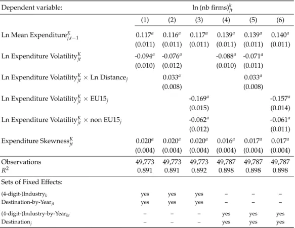
standard errors are clustered at the destination-(4-digit)-industry level. The results reported in Table 2 control for unobserved heterogeneity in industries and destina-tion markets by including the same two sets of fixed effects as in the intensive mar-gin regressions: industry and destination-by-year fixed effects (columns 1 to 3), and industry-by-year and destination fixed effects (columns 4 to 6). As in the intensive margin case, the number of French exporters in a destination-industry-year triplet is positively influenced by the expected demand and the skewness and negatively im-pacted by the volatility. We also document the same trade costs and trade policy ef-fects. The extensive margin of trade is more sensitive to volatility effects in the closest markets and where the trade barriers are the lowest.
3.3
Robustness of industry-level evidence
This section investigates the robustness of the industry-level evidence presented above. Fourth sensitivity tests are performed: i) estimations without skewness, ii) estimations including the average growth of expenditures (in addition to mean expenditure in logs), iii) estimations using alternative measures for expenditure moments based on log differences, and iv) estimations controlling for spatial and serial correlations. Re-garding the last robustness check, we use the method developed byConley(1999) and
heteroskedasticity-Table 2: Extensive margin: Number of exporting firms per industry and uncertainty
Dependent variable: ln (nb firms)kjt
(1) (2) (3) (4) (5) (6)
Ln Mean ExpenditureKj,t−1 0.117a 0.116a 0.117a 0.139a 0.139a 0.140a
(0.011) (0.011) (0.011) (0.011) (0.011) (0.011)
Ln Expenditure VolatilityKjt -0.094a -0.076a -0.088a -0.071a
(0.010) (0.012) (0.010) (0.011)
Ln Expenditure VolatilityKjt×Ln Distancej 0.033a 0.033a
(0.008) (0.008) Ln Expenditure VolatilityK jt×EU15j -0.169a -0.157a (0.015) (0.014) Ln Expenditure VolatilityK jt×non EU15j -0.062a -0.061a (0.012) (0.011) Expenditure SkewnessK jt 0.020a 0.020a 0.020a 0.016a 0.017a 0.017a (0.004) (0.004) (0.004) (0.004) (0.004) (0.004) Observations 49,773 49,773 49,773 49,787 49,787 49,787 R2 0.891 0.891 0.892 0.898 0.898 0.898
Sets of Fixed Effects:
(4-digit-)Industryk yes yes yes – – –
Destination-by-Yearjt yes yes yes – – – (4-digit-)Industry-by-Yearkt – – – yes yes yes
Destinationj – – – yes yes yes
Notes: dependent variable is the logged number of firms per destination-(4-digit-)industry-year triplet. Number of years: 10; Number of destinations: 90; Number of 4-digit industries: 119. Expenditure is defined as apparent consump-tion (producconsump-tion minus net exports) at the 3-digit K level. See the paper for computaconsump-tional details about expenditure moments. Distance is the geographical distance between France and the destination country. EU is a dummy vari-able that equals one for relationships between France and its EU partners. Robust standard errors are in parentheses, clustered by destination-(4-digit-)industry level, withadenoting significance at the 1% level.
and autocorrelation-consistent correction allowing for both spatial and serial correla-tions. As in Berman et al. (2017), we assume that the horizon at which serial correla-tion vanishes can be infinite (e.g., 100,000 years). For the spatial correlacorrela-tion, we select a radius of 4,300 kilometers, which is the median distance between France and all the destination countries included in our sample.
For each robustness check, reported in the online Appendix, the intensive and ex-tensive margin results hold. The magnitude of the volatility estimate is marginally smaller when skewness is omitted, but remains highly significant. By contrast, the magnitude of the volatility estimate is somewhat larger when the average growth of expenditure is added, while the estimates of mean and skewness expenditure are not impacted. Note that the average growth of expenditure has a positive impact on indus-try exports and on the number of exporting firms per indusindus-try. Moreover, the results are valid if expenditure volatility and skewness are computed using log differences in
R instead of growth rates as explained in section2.2.
4
Firm-level evidence
The intensive and extensive margins of trade are now estimated at the firm level (sec-tions4.1and 4.3), while we explore the heterogeneous intensive responses of firms to expenditure volatility in section 4.2.21 The economic meaningfulness of the estimates of volatility and skewness on trade, as well as the rationalization of our findings, are discussed in Section5.
4.1
Intensive margin of trade
We estimate the following specification of firm-level exports at the destination-(4-digit)-industry-year triplet:
ln ykf jt =β1lnEt(RKjt) +β2lnVt( ˙RKjt) +β3St(R˙Kjt) + X0γ+εkf jt, (9)
where ykf jtis now the export value of French firm f to destination j at the 4-digit man-ufacturing level k in year t. As previously described, Et(RKjt), Vt(R˙Kjt), andSt( ˙RKjt)are
the first three central moments of the expenditure distribution, and εkf jtrepresents the usual error term. Compared with the industry-level estimations, firm-level data of-fer considerably more observations and mitigate concerns about the inefficiency of the panel estimator when introducing various combinations of fixed effects. Consequently, we use fairly demanding specifications with a vector X of different combinations of fixed effects. The standard errors are clustered at the destination-(4-digit)-industry level.22
The main results are reported in Table3and presented according to the main source
21As in section3, we focus our analysis on export values and present the analyses on quantities and
prices in the online Appendix.
22We use the Stata package REGHDFE developed byCorreia(2014). Because maintaining singleton
groups in linear regressions where fixed effects are nested within clusters might lead to incorrect infer-ences, we exclude groups containing only one observation (Correia,2015). Therefore, the numbers of observations differ across estimations. The results are similar when retaining singleton groups.
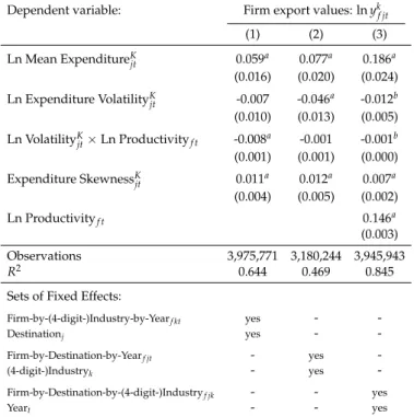
of variation in expenditure: across destination markets (column 1), industries (column 2), and years (column 3). Before discussing the differences across columns, note that in every specification, all coefficients are statistically significant (at the 1 percent con-fidence level) and exhibit the expected signs. The results clearly show that expendi-ture volatility is negatively correlated with firm export values. This finding confirms the industry evidence presented above. Moreover, as expected, average expenditures, skewness, and firm productivity are positively correlated with the export values.
Table 3: Intensive margin: Firm export values
Dependent variable: Firm export values: ln yk
f jt (1) (2) (3) Ln Mean ExpenditureK j,t−1 0.060a 0.077a 0.186a (0.016) (0.020) (0.024) Ln Expenditure VolatilityK jt -0.034a -0.049a -0.015a (0.010) (0.013) (0.005) Expenditure SkewnessK jt 0.012a 0.013a 0.007a (0.004) (0.005) (0.002) Ln Productivityf t 0.147a (0.003) Observations 3,975,771 3,180,244 3,945,943 R2 0.644 0.469 0.845
Sets of Fixed Effects:
Firm-by-(4-digit-)Industry-by-Yearf kt yes - -Destinationj yes - -Firm-by-Destination-by-Yearf jt - yes -(4-digit-)Industryk - yes -Firm-by-Destination-by-(4-digit-)Industryf jk - - yes Yeart - - yes
Notes: dependent variable is firm-level export values in logs aggregated at the 4-digit k level. Number of years: 10; Number of destinations: 90; Number of 4-digit industries: 119; Number of firms: 105,724. Expenditure is defined as apparent consumption (pro-duction minus net exports) at the 3-digit K level. See the paper for computational details about expenditure moments. Robust standard errors are in parentheses and clustered by destination-(4-digit-)industry level, withadenoting significance at the 1% level.
In column 1, we introduce firm-by-industry-by-year fixed effects (αf kt), which
cap-ture all time-varying firm-specific determinants, such as productivity and debt, as well as any firm-industry heterogeneity. The coefficients of interest on volatility and skew-ness are identified in the destination dimension. In other words, the estimation relies on firm-industry-year triplets with multiple destinations. We add a separate desti-nation country fixed effect (αj) to control for destination-specific factors. In this way,
high skewness. This estimation neutralizes the ability of firms to manage their risk exposure by adjusting their (4-digit) industry lines.
In this fixed effects setting, we find a negative effect of expenditure volatility and a positive effect of expenditure skewness on firm-level exports. Hence, multi-destination firms manage their risk exposure by favoring countries with low expenditure variance and high skewness. In other words, firms avoid a high-risk market j by diverting exports to other markets with lower risks.
In column 2, we introduce firm-by-destination-by-year fixed effects (αf jt). With this
specification, we still absorb productivity differences across firms, but we also con-trol for any time-varying firm-destination-specific factors. Our coefficients of interest are now identified in the industry dimension. In other words, the estimation relies on firm-destination-year triplets with multiple 4-digit industries. We add a separate 4-digit industry fixed effect (αk) to control for industry-specific factors. Hence, we
esti-mate whether firms favor the exports of industries with low volatility and high skew-ness for a given destination-year triplet. In this setting, by controlling for firm-by-destination-by-year fixed effects, we eliminate the possibility that firms diversify across destinations. Unsurprisingly, the magnitude of the volatility estimate increases from 0.034 in column 1 to 0.049 in column 2. Firms are more affected because it is intu-itively more difficult to diversify across industries than it is across destinations when uncertainty increases. The magnitude of the skewness effect is also somewhat larger.
In column 3, we use firm-by-destination-by-industry fixed effects (αf jk) and add a
separate year fixed effect (αt). We capture any differences that are maintained across
our observation period at the firm-destination-industry level. However, this set does not control for time-varying firm characteristics such as productivity, which is now in-troduced as an additional control and defined as the ratio of value added to the num-ber of employees. The estimates in the third column have a very natural interpretation with a set of fixed effects corresponding to a within-panel estimator. The identification lies in the variation of expenditure moments over time. The within estimates suggest that, for a given firm-destination-industry triplet, an increase in volatility over time
reduces the firm’s export values, while an increase in skewness increases exports.
4.2
Heterogeneous intensive responses of firms to expenditure
volatil-ity
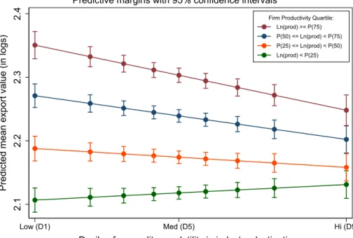
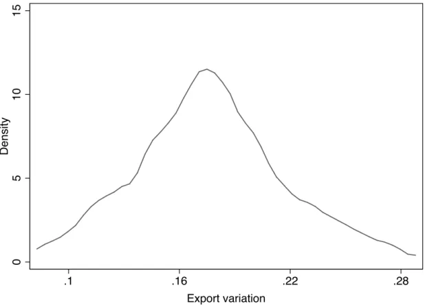
We now assess the potential for heterogeneity in firm responses to volatility on the in-tensive margin of trade. Specifically, we evaluate whether expenditure uncertainty re-duces the difference in export values between the least and the most productive firms. To this end, we first construct Figure5, which depicts a parametric version of the real-location effect.23
To construct Figure 5, we first divide firm productivity into quartiles and indus-try expenditure volatility into deciles. Then, we create new variables by interacting each productivity quartile with the volatility deciles. Finally, we use an estimator that allows us to identify these interactions and to overcome the computational cost of cal-culating the marginal effects. We run the regression by conditioning firm responses on destination-by-year (αjt) and firm-by-(4-digit)-industry (αf k) fixed effects. Based on
the estimated parameters, we compute the predicted mean of export value (in logs) for each decile of volatility and quartile of productivity. The different predictions for trade are plotted in Figure5. This plot shows three interesting results: (i) the most productive firms export more than the others at any level of volatility; (ii) the greater the expen-diture volatility is, the smaller the export values for all levels of productivity, except for the least productive firms; and (iii) the marginal decrease in exports increases for the most productive firms as volatility increases. These results imply that the export difference between the least and the most productive firms decreases with volatility. We find that the 25% most productive firms export, on average, 27% more in value than the 25% least productive firms do in less volatile markets, while this difference decreases to 12% percent in the most volatile markets.
23AppendixCprovides a nonparametric version of this figure, which also documents the reallocation
Figure 5: Volatility, productivity and export values
2.1
2.2
2.3
2.4
Predicted mean export value (in logs)
Low (D1) Med (D5) Hi (D9)
Decile of expenditure volatility in industry-destinations
Ln(prod) >= P(75) P(50) <= Ln(prod) < P(75) P(25) <= Ln(prod) < P(50) Ln(prod) < P(25) Firm Productivity Quartile:
Predictive margins with 95% confidence intervals
Note: The figure compares exporters across categories of productivity (prod) and expenditure volatility in terms of predicted export values between 2000 and 2009. The x-axis displays the deciles of expenditure volatility in 3-digit industry-destination-year triplets. The y-axis displays the predicted mean export value in 4-digit industry-destination-year triplets. See the text for estimation details.
We now pursue our investigation of the heterogeneous responses of firms to expen-diture volatility using the same firm specifications as in Table 3. The only difference is that we add a new covariate to the specifications: the interaction between volatil-ity and firm productivvolatil-ity. The estimates are reported in Table 4. The results confirm that the most productive firms are more sensitive to variation in expenditure volatility (across destinations, industries, and years). High productivity firms export less in the most volatile markets.
4.3
Extensive margin of trade
We now investigate the impact of uncertainty on the extensive margin of trade. We follow the same identification strategy as above, with a disaggregated left-hand side variable regressed on the aggregated right-hand side expenditure moments. We dis-tinguish between the entry of new French firms into the international market and the exit of incumbents from that market over the 2000-2009 period. Regarding entry, our
Table 4: Intensive margin: Reallocation of exports across firms
Dependent variable: Firm export values: ln yk f jt (1) (2) (3) Ln Mean ExpenditureK jt 0.059a 0.077a 0.186a (0.016) (0.020) (0.024) Ln Expenditure VolatilityK jt -0.007 -0.046a -0.012b (0.010) (0.013) (0.005) Ln VolatilityK jt×Ln Productivityf t -0.008a -0.001 -0.001b (0.001) (0.001) (0.000) Expenditure SkewnessK jt 0.011a 0.012a 0.007a (0.004) (0.005) (0.002) Ln Productivityf t 0.146a (0.003) Observations 3,975,771 3,180,244 3,945,943 R2 0.644 0.469 0.845
Sets of Fixed Effects:
Firm-by-(4-digit-)Industry-by-Yearf kt yes - -Destinationj yes - -Firm-by-Destination-by-Yearf jt - yes -(4-digit-)Industryk - yes -Firm-by-Destination-by-(4-digit-)Industryf jk - - yes Yeart - - yes
Notes: dependent variable is firm-level export values, in logs and aggregated at the 4-digit k level. Number of years: 10; Number of destinations: 90; Number of 4-4-digit indus-tries: 119; Number of firms: 105,777. Expenditure is defined as apparent consumption (production minus net exports) at the 3-digit K level. See the paper for computational details about expenditure moments. The productivity of firm f in year t is measured us-ing the value-added per employee. Robust standard errors are in parentheses, clustered by destination-(4-digit-)industry level, withaandbdenoting significance at the 1% and 5% level respectively.
dependent variable (ykf jt) is the probability that firm f begins exporting to destination j in 4-digit industry k and year t. Our counterfactual scenario considers the firms that do not enter in the same triplet jkt. This choice model can be written as a latent vari-able representation, with y∗f jtk being the latent variable determining whether a strictly positive export flow is observed for firm f in a destination-industry-year triplet. Our estimated equation is therefore:
Pr(ykf jt|ykf j,t−1 =0) = 1 if y∗f jtk >0, 0 if y∗f jtk ≤0, (10) with y∗f jtk =λ1lnEt(RKj,t) +λ2lnVt(R˙Kjt) +λ3St(R˙Kjt) +X0γ+εkf jt,
where, as previously described,Et(RKjt),Vt(˙RKjt), andSt( ˙RKjt)are the first three central
effects; and εkf jtis the error term. In addition to the probability of entry, one can study the exit transition. Higher volatility or lower upside gains may increase the exit of firms from the export market. In the exit case, our dependent variable is the probability that firm f in destination j, industry k and year t−1 stops exporting products from industry k to this destination in year t. Our counterfactual scenario now considers the firms that continue to serve the same triplet jkt. The explanatory variables are the same as in the entry estimations.
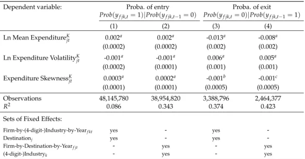
We estimate the entry and exit equations using a linear probability model (LPM). The inclusion of fixed effects in a probit model would give rise to the incidental param-eter problem. The LPM avoids this issue. Furthermore, the use of an LPM allows us to directly interpret the coefficients. As for the intensive margin, in all regressions, we account for the correlation of errors by clustering at the destination-(4-digit-)industry level. The results are reported in Table5.
In accordance with the definition of our counterfactual scenarios, we investigate the effects of uncertainty across industries and destinations. In columns 1 and 3, we introduce destination (αj) and firm-by-industry-by-year (αf kt) fixed effects. Here, our
coefficients of interest on volatility and skewness are identified in the destination di-mension. In other words, regarding the probability of firm entry (column 1), we com-pare firms in a given industry k and year t entering an export market j versus those not entering that market. In columns 2 and 4, we introduce industry (αk) and
firm-by-destination-by-year fixed effects (αf jt). Our coefficients of interest on volatility and
skewness are now identified in the industry dimension. Regarding the probability of firm entry (column 2), we compare firms in a given destination j and year t entering industry k versus those not entering that industry.24
Table 5 presents quite intuitive results. Mean expenditure significantly increases the probability that a firm enters a destination j or an industry k (columns 1-2), while reducing the probability of exit (columns 3-4). As expected, the within
firm-industry-24Given the definitions of entry and exit, which are based on yearly firm behaviors in each
destination-industry, the investigation of the variation across years at the firm-destination-industry level is not as relevant as on the intensive margin. Therefore, we do not consider for the extensive margin a specifica-tion with firm-by-destinaspecifica-tion-by-industry fixed effects (αf jk) or a separate year fixed effect (αt).
year (columns 1 and 3) and firm-destination-year (columns 2 and 4) dimensions react to the second- and third-order moment changes in expenditures. Expenditure volatil-ity significantly decreases the probabilvolatil-ity of entry and increases the probabilvolatil-ity of exit. These results depict the reallocation effects across destinations and industries in terms of export decisions. Interestingly, destination reallocation appears to be stronger (see columns 1 and 3 versus columns 2 and 4). As noted for the intensive margin of trade, diversification and reallocation across destinations is easier than diversification across industries, which may explain the difference in the magnitudes of the coefficients. Thus, a smaller volatility effect on the intensive margin is consistent with a larger effect on the extensive margin. Note that skewness has a positive and significant effect on the probability of entry and a negative and significant impact on the probability of exit.
Table 5: Extensive margin: Firm entry and exit probabilities
Dependent variable: Proba. of entry Proba. of exit
Prob(yf jk,t=1)|Prob(yf jk,t−1=0) Prob(yf jk,t=0)|Prob(yf jk,t−1=1)
(1) (2) (3) (4) Ln Mean ExpenditureKjt 0.002a 0.002a -0.013a -0.008a (0.0002) (0.0002) (0.002) (0.002) Ln Expenditure VolatilityKjt -0.001a -0.001a 0.006a 0.005a (0.0002) (0.0001) (0.001) (0.001) Expenditure SkewnessKjt 0.0003a 0.0002a -0.001b -0.001c (0.0001) (0.0001) (0.0005) (0.0005) Observations 48,145,780 38,954,820 3,388,796 2,464,377 R2 0.086 0.343 0.374 0.423
Sets of Fixed Effects:
Firm-by-(4-digit-)Industry-by-Yearf kt yes - yes
-Destinationj yes - yes
-Firm-by-Destination-by-Yearf jt - yes - yes
(4-digit-)Industryk - yes - yes
Notes: dependent variable is probability for a firm to enter the export market (columns 1-2) and probability for a firm to exit the export market (columns 3-4). Entry sample: 9 years, 89 destinations, 119 4-digit industries, and 75,791 firms. Exit sample: 9 years, 89 destinations, 119 4-digit industries, and 73,270 firms. Expenditure is defined as apparent consumption (production minus net exports) at the 3-digit K level. See the paper for computational details about expenditure moments. Robust standard errors are in parentheses, clustered by destination-4-digit industry level, witha,b, andcdenoting significance at the 1%, 5%, and 10% level respectively.
4.4
Robustness of firm-level evidence
In this section, we check the robustness of the intensive and extensive firm-level results. First, AppendixDshows that our results are robust to the consideration of mono- and multi-destination firms as well as mono- and multi-industry firms.
Second, we test whether our estimates are impacted when i) omitting the skewness, ii) including the average growth of expenditures (in addition to logged-mean expendi-ture), iii) using alternative measures of expenditure moments based on log differences, and iv) considering the export quantities or the export prices as the dependent vari-ables instead of the export values.25 These robustness checks, reported in the online Appendix, do not alter our main conclusions.
We also study the sensitivity of our results to alternative definitions of entry and exit. The definitions used in Section4.3may capture small exporters that enter and exit the international market several times over the sample period (2000-2009). Requiring that a firm entering the export market in year t remains in t+1 and, similarly, that a firm exiting the export market in year t remains a nonexporter in t+1 does not affect the estimation results.
In addition, we show that our results are not driven by the time span chosen for the construction of the expenditure moments, e.g. 5- and 7-year rolling periods instead of a 6-year time window (see the online Appendix).
Finally, in addition to removing French export and import flows from the destina-tion’s expenditure computation (see2.2), we exclude industry-destination pairs where France has a significant market share. In particular, we drop from each regression, reported in the online Appendix, the industry-destination pairs belonging to the top 10% of the destination’s expenditure distribution. In this top decile, French exports represent at least 4% of the destination’s total expenditure. The results remain nearly unchanged from the baseline results displayed in Table3.
5
Discussion and simulations
Our estimations reveal that expenditure volatility negatively affects both the inten-sive and exteninten-sive margins of trade. The estimations also highlight the heterogeneous
25Unfortunately, serial correlation cannot be tested at the firm level because the firm sample size is far
too large relative to the computing power required to run the programs. However, as previously shown at the industry level, our results do not appear to be significantly affected by spatial and temporal correlations.
effects of uncertainty. The more-productive exporters seem to favor destinations or industries with low volatility. By contrast, the less-productive exporters can increase their exports in the countries and industries with high volatility due to the reallocation of market shares among firms. Our results on expenditure skewness also suggest that downside risk matters to exporters.
5.1
How economically meaningful are the estimates of volatility and
skewness?
To answer this question we evaluate the expected change in export value at the indus-try level if all countries exhibit the lowest level of volatility observed across destina-tions Vmink ≡ min Vjtk for a given industry k. We also decompose the expected change into extensive and intensive margin changes. To implement this counterfactual analy-sis, we use the results associated with the estimation of two equations: first the number of exporters in a destination-industry-year triplet (equation8) and, second, firm-level export values at a destination-industry-year triplet (equation9).
Assuming for simplicity that Skjt=0, the expected change in the value of exports in a destination-industry-year triplet,∆vkjt, can be written as follows
∆vk jt≡ne k tve k t −nkjtvkjt
where nkjt and vkjt represent the observed number of exporters and average exports, respectively, and ne
k
t and ve
k
t represent the expected number of exporters and average
exports, respectively, when the level of volatility prevailing in destination country j and industry k reaches Vmink (with Skjt=0).
As industry-level French trade vkjt = nkjtvkjt can be decomposed into an extensive margin, nkjt, and an intensive margin, vkjt, the expected change∆vkjtis also given by
∆vk