The Simulation of the Educational Output over the Life Course: The GAMEO Model

HAL Id: hal-00391393

https://hal.archives-ouvertes.fr/hal-00391393

Submitted on 3 Jun 2009

HAL is a multi-disciplinary open access

archive for the deposit and dissemination of sci-entific research documents, whether they are pub-lished or not. The documents may come from teaching and research institutions in France or abroad, or from public or private research centers.

L’archive ouverte pluridisciplinaire HAL, est destinée au dépôt et à la diffusion de documents scientifiques de niveau recherche, publiés ou non, émanant des établissements d’enseignement et de recherche français ou étrangers, des laboratoires publics ou privés.

The Simulation of the Educational Output over the Life

Course: The GAMEO Model

Pierre Courtioux, Stéphane Gregoir, Dede Houeto

To cite this version:

Pierre Courtioux, Stéphane Gregoir, Dede Houeto. The Simulation of the Educational Output over the Life Course: The GAMEO Model. 2nd general conference of the International Microsimulation Association : “Microsimulation: Bridging Data and Policy”, Jun 2009, Ottawa (Ontario), Canada. �hal-00391393�

1

Paper presented at the 2nd general conference of the International Microsimulation Association :

“Microsimulation: Bridging Data and Policy”

June 8th to 10th 2009, Ottawa (Ontario), Canada

The Simulation of the Educational Output

over the Life Course: The GAMEO Model

Pierre Courtioux

, Stéphane Gregoir

, Dede Houeto

8th June 2009

Acknowledgments

The estimates used for microsimulation in this paper are done on three sets of data: the French Labour Force Survey for 2003-2005, which is available online (http://www.insee.fr), the French Labour Force Survey 1968-2002, which is available for researchers from the Quetelet Centre (http://www.centre.quetelet.cnrs.fr/), and the mortality rates and their forecast based on Vallin and Meslé (2001) and Robert-Bobée (2006). The model used for the simulations is developed at EDHEC’s Economics Research Centre; the version presented here is GAMEO V1.3.

1

EDHEC Business School.

2 _{EDHEC Business School.}

3 _{EDHEC Business School and Paris School of Economics.}

hal-00391393, version 1 - 3 Jun 2009

Author manuscript, published in "2nd general conference of the International Microsimulation Association : “Microsimulation: Bridging Data and Policy”, Ottawa (Ontario) : Canada (2009)"

2

1. Introduction

When one considers public policies, investing in education seems to be a crucial issue at stake in developed countries. For instance, the European Lisbon Strategy and its educational part— the so-called Education and Training 2010—put the stress on the link between education system and social cohesion and establish some educational targets like the share of early school leavers, the increase in the part of graduates in master of science and technology, etc4. More recently in the United-States, the American Recovery and Reinvestment Act points out the need of heavily investing in education to “provide jobs now and lay the foundation for long-term prosperity”; it focuses notably on early childhood education and higher education. In this framework, from a micro point of view it is important to identify the different contributors and beneficia ries of these policies. On the one hand, contributors may include the State—and tax payers—by way of subsidies to education policy in various way—public subsidies for schools, guarantee for student loan, etc. —, consumers of education —students, etc. — and their families by mean of tuition fees and/or taxes. On the other hand, the return to this education investment is captured by the graduates —mainly by ways of a wage premium—, but also by the State insofar as the wage premium of graduates leads to an increase in taxes, and that there exists some externalities which would increase the productivity of the whole economy.

According to the traditional approach in education economics, education can be considered as a part of human capital that impacts earnings over the course of a lifetime. The gains of this investment can be assessed by computing the individual internal rate of return of one additional year of education. Since the seminal Mincer (1974) study, measuring the internal rate of return to education has become an important dimension of the analysis of education choices, which emphasize controlling for endogeneity—Heckman et al. (2006). A complementary approach, still underdeveloped in education economics, is the dynamic microsimulation method that attempts to take into account the complexity of national socio-fiscal regimes—for instance, Harding (1993), Mitton et al. (2000). This method enables to simulate the diversity of careers in a given tax and transfer regime: basically, the micro-units are considered one year older at each new step of the simulation. This ageing process affects the probability of changing labour market positions, wages and the corresponding taxes and transfers. When education economics are considered, the advantage of a dynamic

4 _{For more details, see Commission of the European Communities (2005).}

3

microsimulation approach is that it includes in the calculation of the internal rate of return to education the whole tax and benefit system: for instance, a more complete calculation of the internal rate of return to education can be produced if pension schemes and more generally the last part of the lifetime are taken into account. The microsimulation approach enables an analysis of the distribution of the internal rates of return to education for a given diploma. From this point of view, the development of a dynamic microsimulation model is important to analyse education policy as an investment, to identify the winners and the losers, as well as the macro revenues of these investments that have to be considered over a lifetime. The evaluation of these policies has to take into account the socio- fiscal regime but also the specificities of the national education system. For instance, there is an analytical tradition in socio-economics5 which links education system and the occupation and status on the workplace and/or the labour market. In the current appraisal of education in economic microsimulation, individual education is often represented by the schooling years’ number. The objective of the model presented in this paper is to go further and to present a more comprehensive approach of the link between education and the labour market. This comprehensive approach takes into account the different diplomas produced by the French education system and the careers they lead to.

In this paper, we present the GAMEO6 model, which is currently developed at the Economic Research Center of EDHEC Business School. GAMEO is a dynamic microsimulation model with two main features: (i) it proposes a very precise appraisal of education in France; (ii) it focuses on the life course of a given generation. The model is coded with SAS; it has three parts. The first part GAMEO-A aims at producing an artificial input data representing a chosen generation in terms of gender, diploma and age entering the labour force. GAMEO-A input to produce simulated samples is the French Labour Survey 2003-2005. The number of observations in the input data can be calibrated in order to make a trade-off between precision of risk analysis and the calculation time. The second part, GAMEO-B, aims at producing individual income paths. It simulates the transition between various positions (employment, unemployment, inactivity) and the associated income (wage, unemployment benefit, retirement pension) as well as some other elements of the socio- fiscal system (income tax).

5

For instance, the seminal work of Maurice and alii (1982). Gazier and Schmid (2002) and Schmid (2006) are more recent work close to this analytical tradition which put the stress on the methodology for international comparisons of labour market and social policies and the way to deal with institutions.

6 _{GAMEO stands for Generational Accounting and Microsimulation of Educational Output.}

4

The third part GAMEO-C aims at computing individual internal rates of return to education, based on the different individual simulated trajectories.

In section 2, we present the way our microsimulation model apprehend the particularity of the French education system and its impact on individual trajectories. In section 3, we detail the simulation of individual position vis à vis the labour market over their lifetime. In section 4, we examine the way the individual income is imputed. In section 5, we explain the way we capture individual life expectancy.

2. How to apprehend French education system and its monetary outputs

In section 2.1, we present the specificities of the French education system which is characterized by a structural opposition between the grandes écoles system and the university; the way the French Labour Force Survey (FLFS) 2003-2005 enables us to apprehend this education diversity is also presented. The section 2.2 explains how it is possible to increase the number of diplomas’ categories taken into account in the input data base of GAMEO. We present a modelling strategy which enables us to differentiate the elite schools engineers from the engineers graduated from other grandes écoles. The section 2.3 explains how it is possible to take into account the specificities of French education system on the basis of the French Labour Force Survey (FLFS) 2003-2005 to simulate individual trajectories with an important heterogeneity in diploma for a given generation.

2.1. The French education system: some stylized facts

In France, school is compulsory until the age of sixteen. There are some mid-school professional degrees for those who choose to enter early the labour force: the Certificat

d’Aptitude Profesionnelle (CAP) and the Brevet d’Etudes Professionnelles (BEP). At the end

of the High School there is an exam, the so-called Baccalauréat which it is necessary to pass in order to enrol in higher education7. There are three main types of Baccalauréat8: the

7 _{There is one exception the Capacité en droit is a higher education diploma in law. This curriculum is also open}

to those who do not passed the Baccalauréat.

5

general ones—which are declined with a given set of majors—and two specialized

Baccalauréat —a professional one and a technical one.

France is particular when one considers the great heterogeneity of tertiary education paths— see diagram 2.1—and of their corresponding costs. This heterogeneity goes beyond the evidence that scientific programmes of study are generally more costly than other programmes, and relates to the different institutions in charge of higher education paths and their place in the educational system.

Traditionally, at the end of high school, students have to choose between two paths: the State universities and the higher education institutions known as grandes écoles. The universities are a quasi no-charge system whatever the subject area chosen by the student. The grandes

écoles involve two steps. The first step consists of two years in a State-subsidized preparatory

class (Classe préparatoire aux grandes écoles) that is free of charge. The second involves three years in a grande école. For this second step the choice of the student subject area has financial consequences: engineering schools are subsidized by the State, whereas business schools are much less heavily subsidized and charge their students high fees. There is a traditional ranking of the grandes écoles which lead to identify a sub-group of elite schools. The range of this elite school category is difficult to identify clearly; from a statistical point of view, the ‘the French Labour Force Survey 1990-2002 identify an ad hoc specific class for elite school that has been abandoned in the more recent surveys—see section 2.2.

Aside from these two traditional main paths, there are some other specific diplomas: a two-year technical one known as a BTS (Brevet de Technicien du Supérieur) and offered by technical schools, the DUT (Diplôme Universitaire de Technologie) and the DEUST (Diplôme d’Etude Universitaire Scientifique et Technique); these last two are two- year specialized degrees offered at some universities.

Public expenditures for a student in France are thus closely related to the student’s higher education path. These differences stem mainly from staff spending: preparatory classes and

grandes écoles offer small classes, whereas university teaching is generally done in large

lectur e halls.

In France, few statistics are available on the real cost of training when one considers the diploma obtained. However, Zuber (2004) proposes an evaluation of the mean costs of the higher education diploma for the State.

8 _{See diagram 2.1.}

6

Differences in individual higher education costs stem from the number of years of education, the education path and the major. The cost of an additional year of higher education differs greatly according to the education path. The average cost per year for a two-year university diploma is 2,453 euros, whereas the average cost per year for an engineering school diploma is nearly five times higher. When we also consider the years in preparatory schools, the total cost of an engineering school diploma is twelve times higher. This difference is only partially explained by the increasing cost of a year of higher education with the level of education. When one considers the same level of education, engineering school costs are more than three times higher than the same level university degree.

When one considers the elite schools, the subsidized cost is more than sixteen times higher than that of a five- year university degree. One can argue that the costlier scientific curriculum of engineering schools accounts for these differences. However, according to Zuber (2004), the differences in costs remain. If one considers only scientific university programs, engineering schools are still one and a half times more costly

7

Diagram 2.1. The French education system

The FLFS 2003-2005 contains a variable which identifies the higher diploma obtained. It enables us to retain twenty classes of diploma:

1- No diploma. 2- CAP/BEP.

3- Baccallauréat Général. 4- Baccallauréat Professionnel. 5- Baccallauréat Technique. 6- Capacité en droit (University). 7- DEUG (University).

8- DUT or DUST (University). 9- BTS.

10- Higher educated technician diploma.

8 11- Paramedical diploma.

12- Licence (University).

13- Other three-years graduate degree. 14- Maîtrise (University).

15- DEA (general master at University). 16- DESS (professional master at University). 17- Master of Business Schools.

18- Master of Engineering Schools.

19- Doctorat (PhD), medical degree (University). 20- Doctorat (PhD), other major (University).

One important limit of this classification of diploma is that it is not possible to identify the graduated from elite Schools which concerns mainly engineering Schools. The following section explains the modelling strategy chosen to take into account the graduates from elite schools in the GAMEO model.

2.2. Determining elite school’s graduates in the input data

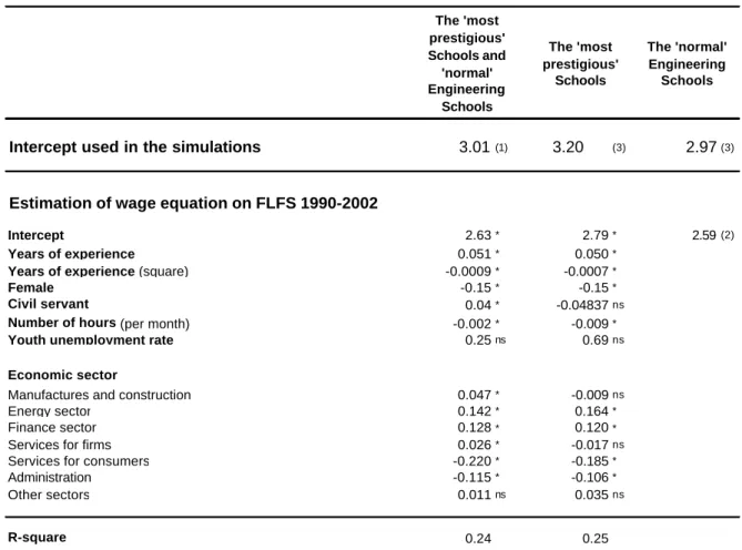
In the FLFS 2003-2005 there are no data on the elite schools of the French higher education system. However, for the FLFS 1990-2003 it is possible to identify some individuals with a degree from the ‘most prestigious’ grandes écoles. It is an ad hoc classification, some classes of which mix engineers, but also some law schools, and other elite schools mainly for civil servants —Ecole nationale d’administration,Ecole normale supérieure, Science Po, etc.9 When one estimates an earning equation with the FLFS 1990-2002, first for the ‘most prestigious’ schools and then for these schools and the other engineering schools, one could note that the main difference concerns the intercept of the equation, which is higher for the ‘most prestigious’ schools (table 2.1), and the coefficients, which are not directly comparable with those of the equation estimated on the FLFS 2003-200510—this could be the result of a major change in data collection in 2003.

9 _{For a description of this class, see Albouy and Wanecq (2003).}

10 _{See section 4, table 4.1 for the detailed estimates based on the FLFS 2003-2005.}

9

It is possible to estimate a wage equation for the ‘most prestigious’ engineering schools for the period from 2003 to 2005, making the following assumptions: 1) the elite engineering schools do not differ from the ‘most prestigious’ higher education schools category considering the coefficients estimated in the wage equation; 2) only the level of the intercept differs when one considers the wage equation coefficients of the graduates of the elite schools and those of the graduates of normal schools; 3) the proportion between the intercepts is the same whatever the period considered.

Table 2.1. Estimation of earning functions for different types of engineers

Intercept used in the simulations 3.01(1) 3.20 (3) 2.97(3)

Estimation of wage equation on FLFS 1990-2002

Intercept 2.63* 2.79* 2.59(2)

Years of experience 0.051* 0.050*

Years of experience (square) -0.0009* -0.0007*

Female -0.15* -0.15*

Civil servant 0.04* -0.04837ns

Number of hours (per month) -0.002* -0.009*

Youth unemployment rate 0.25ns 0.69ns

Economic sector

Manufactures and construction 0.047* -0.009ns

Energy sector 0.142* 0.164*

Finance sector 0.128* 0.120*

Services for firms 0.026* -0.017ns

Services for consumers -0.220* -0.185*

Administration -0.115* -0.106* Other sectors 0.011ns 0.035ns R-square 0.24 0.25 The 'most prestigious' Schools and 'normal' Engineering Schools The 'most prestigious' Schools The 'normal' Engineering Schools

Source: French Labour Force Survey 1990-2002 (Insee)—authors’ calculation.

Note: (*) for 1% and (ns) for no significance. (1) This intercept corresponds to the one which is presented in table 4.1, last column, (2) this

intercept could be computed from the two other intercepts and the probability of being from a ‘most prestigious’ school (19.9%), (3) this intercept is computed from the intercept estimated with the FLFS 1990-2002 and from the intercept for engineers’ wage equation whatever the type estimated with the FLFS 2003-2005.

After determining the way to simulate the engineers’ wages by pedigree, as it were, it is important to determine the type of the engineers —elite versus normal —in the input data of the GAMEO model. With our input data constituted with the FLFS 2003-2005, it is not

10

possible to know the provenance of the degrees of the engineers. We decided to duplicate each engineer observation (one for the elite schools, one for the others) and to modify their weight according to their individual probability of being of one particular type

Diagram 2.2 illustrates how this differentiation is obtained: we randomly affect the non explained part of the wages11 which enables us to compute a potential wage; the probability of having graduated from an elite school is then computed based on individual characteristics; the engineer observation is duplicated—one elite and one normal—; the weights of these two new observations, which replace the former one, are corrected based on the probability of having graduated from an elite school.

Diagram 2.2. Construction of elite school’s engineers in the input data of GAMEO

11 _{This wage residual stems from the current GAMEO determination of wages described in the section 4.2.}

11

More precisely, the individual probability—Ei in diagram 2.2 — is estimated as follows.

First, we simulate a wage for the individual:

i i i X u

Y =β +

Where Y is the log of the wage simulated, i β the coefficients of the engineer’s wage equation

presented in table 4.112,X the individual characteristics and i u a residual drawn from the i

residual pool obtained with the estimation of the engineer wage equa tion using FLFS 2003-2005 data. The conditional probability (under a Gaussian assumption) of having graduated from an elite engineering school is then computed, using the wage equation for this type of engineer.

(

)

where σ is the standard deviation of the wages of a graduate of the elite engineering school, ₁ —the standard deviation is computed using the FLFS 1990-2002—, and β the coefficients of ₁ the wage equation retained for the engineers graduates of the elite school. The conditional probability of an engineer having graduated from another school can then be written:

(

)

where σ is the standard deviation of wages of a graduate of a normal engineering school —₂ the standard deviation is computed using the FLFS 1990-2002—, and β the coefficients of ₂ the wage equation retained for the engineers graduates of a normal school. If we assume that

12 _{It is worth noticing that it mimics the current process of wage determination with GAMEO which is detailed in}

section 4.1.

12

the statistical structure of the population is the same and that the proportion of engineers

graduating from the elite school is the same for the two periods (PPES), we can compute an

estimation of an individual’s probability of having graduated from one of the ‘most

prestigious’ schools (PPESi) as follows (Bayes’ rule):

(

)

This probability is weighted with a coefficient to align the proportion of individuals with a

diploma of an elite engineering school to the observed proportion in the 1990-2002 period

(19.9%).

2.3. Education output as a dynamic process: an overview

The process of a GAMEO simulation is illustrated in the diagram 2.3.

The input data base is produced by GAMEO-A. It represents the individuals of chosen generation with their characteristics as they appeared in the FLFS 2003-2006. To illustrate the simulations with GAMEO throughout the paper, we present some results stemming from Courtioux (2008, 2009), Courtioux and Houeto (2009) which focus on the 1970’s generation. These papers are based on the simulation of 34,643 individuals who represent the individuals born in 1970—around 850,000 people—in terms of sex, diploma and age upon entry into the labour force. The relative percentage of each case is approximated on the basis of the French Labour Force Survey (FLFS) 2003-2005 considering the people born between the 1968 and 1972. The economic sector is determined for the lifetime. It is affected randomly on the basis of the distribution of economic sector of the individual aged 16 to 30 in the FLFS 2003-2005 by gender and diploma.

The modelled ageing process simulates the annual individual transitions between three main states: inactivity, employment and unemployment—for more detail see section 6.2. The simulation begins at sixteen, the legal age for the end of compulsory schooling. A Mincer

13

equation estimated by diploma is used to simulate the wage for those in employment. The equations corresponding to the transition process and the wage simulation are estimated on the FLFS 2003-2005. We then simulate the main features of the French socio- fiscal regime: unemployment benefits, retirement pensions and income tax—see section 4.3 for more details. The probability to survive is calculated until the individual is 100—we then assume that he dies.

Diagram 2.3. The ageing process in the GAMEO model

3. The simulation of the labour market positions over the life course

One of the aims of GAMEO model is to simulate the distribution of individual position vis à

vis the labour market by diploma over their life course. As explained in the introduction, we

retain a generational approach. This methodological choice leads to differentiate the macro

14

destiny of a given generation and the impact of individual education on the distribution of the positions open to this generation.

Section 3.1 explains how the macro targets of the different position at a given age for a given generation vis a vis the labour market are estimated. Section 3.2 explains how it is possible to estimate the impact of a given diploma on the probability of transition to a given position. Section 3.3 explains how the two former elements are used in the microsimulation process.

3.1. Generational profile of activity and unemployment

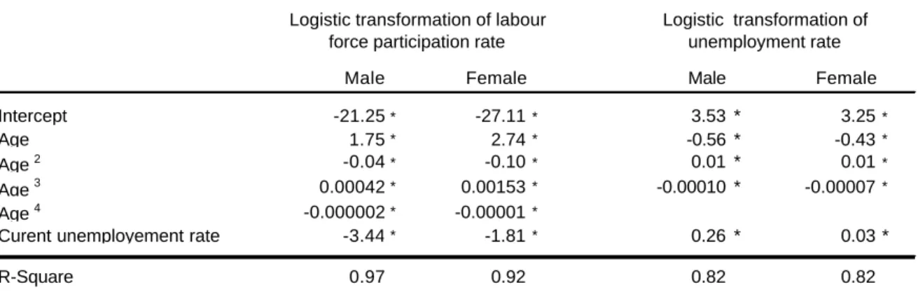
A first step consists in modelling the labour force participation rate and the unemployment rate over the life course for a given generation. The French Labour Force Survey 1968-2005 is used to construct segments of labour participation rate and unemployment rate by age and generation. For instance, data available for the generation born in 1950 cover the ages 18 to 55 which constitutes a segment of life, the generation born in 1960 from the age 16 to 45 –this constitutes another segment-, the generation born in 1970 from 16 to 35, etc. The model is estimated separately for males and females; it includes several specifications for age, the current unemployment rate for a generation at a given age and generation dummies. The equations estimated are specified as follow:

Dg Ut g t g t g t g t P P gt gt + + − + − + − + − + = − 4 3 2 ) ( ) ( ) ( ) ( ) 1 log( α β χ δ ϕ

where P_gt is the participation rate of the generation g for the year t, U the unemployment rate and D a generation dummy.

Dg Ut g t g t g t U U gt gt + + − + − + − + = − 3 2 ) ( ) ( ) ( ) 1 log( α β χ δ

where U_gt is the unemployment rate of the generation g for the year t, U the unemployment rate and D a generation dummy. The main results of the estimations are presented in table 3.1.

15

Table 3.1. Estimation of labour force participation and unemployment rate models

Male Female Male Female

Intercept -21.25* -27.11* 3.53 * 3.25*

Age 1.75* 2.74* -0.56 * -0.43*

Age 2 -0.04* -0.10* 0.01 * 0.01*

Age 3 0.00042* 0.00153* -0.00010 * -0.00007*

Age 4 -0.000002* -0.00001*

Curent unemployement rate -3.44* -1.81* 0.26 * 0.03 *

R-Square 0.97 0.92 0.82 0.82

Logistic transformation of labour force participation rate

Logistic transformation of unemployment rate

Source: Labour Force Survey 1968-2005 (Insee)— authors’ calculation.

Note: taking 1970 for reference, this model is estimated with dummies for each generation; they are not

reproduced here; (*) for 1% level of significance.

3.2. Transition probability and the education effect

In the microsimulation model, the transitions between inactivity, employment and unemployment are modelled. More precisely, five states are modelled: inactivity, self-employment, employment in public sector, employment in private sector and unemployment. We are then interested in the modelling of the following conditional transition probability:

) 1 (a_it =

P where a is the probability of being in activity at the t period, _it P(s_it =1 a_it =1) where s is the probability of being self-employed at the t period, _it P(p_it =1/a_it =1,s_it =0) where p is the probability of being employed in the public sector at the t i_t

period,P(eit =1/ait =1,sit =0,pti =0)where e is the probability of being employed in the it

private sector at the t period.

The individual probability of transition is calculated using binomial logit models, which are estimated on the French Labour Force Survey 2003-2007. The variables used in the model include the former position—which explains an important part of the transition probability13—, some variables describing the socio-economic status, and diploma. The equation estimated is the following:

it it t i it Y S D Y =α +β ₍₋₁₎ +δ +ϕ 13 _{See table 3.2.}

16

where Y is the transition estimated, S a matrix of socio-economic variables and D the i

diploma. The results are presented in table 3.2. It should be noted that the variables used in the estimation of the various equations needed to model individual transitions are not all included in the equations us ed to simulate the individual trajectory. The socio-economic variables concerning the family’s position –number of children if female, young children if female- are included in the estimations to capture their impact on individual transitions on the labour market. They are not however included in the microsimulation of individual transitions: since our analysis is restricted to single individuals, the use of these variables is not warranted.

17

Table 3.2. Estimation of transition models

Intercept 0.261 * 2.196 * 1.434 * 2.108 *

Former position

Inactive ref -5.438 * -5.336 * -1.834 *

Unemployment 2.489 * -6.610 * -6.341 * -3.091 * Self-Employment 5.057 * ref -5.555 * -1.834 * Employment (public sector) 4.166 * -10.020 * ref -1.874 * Employment (private sector) 3.794 * -8.122 * -6.326 * ref

Socio-economic status

Female -0.230 * -0.601 * 0.548 * -0.072 *

Number of Children (if female) -0.089 * 0.066 * 0.008 * -0.091 * Young Children (if female) -1.579 * 0.126 * 0.143 * 0.101 * Age 55 and more -1.491 *

Age 60 and more -1.373 * Age 65 and more -0.352 *

Years of experience -0.018 * 0.040 * 0.067 * 0.045 * Years of experience (square) -0.00003 * -0.001 * -0.001 * Out of the Labour force duration (in years) -0.365 *

Long term unemployment -13.459 ** -16.551 *

Diploma

No Higher Education Diploma

CAP/BEP 0.354 * -0.054 * 0.553 * 0.300 * Bac Général 0.262 * 0.359 * 0.500 * 0.337 * Bac Professionnel 0.914 * 0.295 * 0.083 * 0.653 * Bac Technique 0.495 * 0.056 * 0.593 * 0.451 * Capacité en Droit (1) 0.934 * 0.163 ** -0.841 * -0.396 * Two-year degree DEUG (University) 0.078 * 1.036 * 0.470 * 0.124 * DUT/DEUST (University) 0.772 * -0.285 * 0.275 * 0.848 * BTS 0.617 * 0.471 * 0.008 ns 0.681 *

Other Higher Technician Diploma 0.068 * 0.691 * 0.110 * -0.042 * Paramedical Diploma 0.376 * 2.421 * 3.606 * 1.121 * Three-year degree

Licence (University) 0.139 * 0.576 * 1.212 * 0.272 * Others three-year degree 0.739 * 0.905 * 0.302 * 0.613 * Four-year degree Maîtrise (University) 0.314 * 0.637 * 0.844 * 0.202 * Five-year degree DEA (University) 0.511 * 0.242 * 0.826 * 0.190 * DESS (University) 0.859 * -0.112 * 0.429 * 0.391 * Business Schools 1.164 * -0.464 * -0.626 * 0.529 * Engineering Schools 0.827 * 0.671 * 0.151 * 0.634 *

Degree of more than five years

PhD (Medical Degree excluded) 0.935 * 0.344 * 1.362 * 0.422 * PhD (Medical Degree) 0.694 * 0.796 * 3.223 * 1.205 *

Sommers' D 0.955 0.958 0.911 0.72

P. Conc. 97.7 97.6 95.2 85.6

P. Disc. 2.2 1.9 4.2 13.5

P. Tied 0.1 0.5 0.6 0.9

(public sector) (private sector) Transition to activity Transition to self-employment Transition to employment Transition to employment

Source: French Labour Force Survey 2003-2005 (Insee) – authors ’ calculations.

Note: (*) for 1% and (**) for 5% level of significance. (1) Capacité en droit is a university law degree which

does not imply earlier success on the Bac; it concerns almo st 0.7% of the 1970 generation.

18

3.3. Simulating transitions over a lifetime

In the microsimulation model, the transitions between inactivity, employment and unemployment are modelled. More precisely, five states are modelled: inactivity, self-employment, employment in the public sector, employment in the private sector and unemployment.

The microsimulation of transitions over a lifetime replicates the same pattern for each year— see diagram 3.1. It proceeds as follows. First, the probability of transition to the position of activity is calculated, a random variable is drawn from a uniform probability law on the unit segment and the status—active versus inactive— is selected depending on the realized value of the random variable.. This resolution includes a global alignment to the generation’s rates, the calculation of which was described in section 3.1. Then, knowing that the individual is active, the probability of being self-employed is calculated and a similar procedure applies. Then, knowing that the individual is active and not self-employed, the probability of being in employment in the public sector is calculated and a similar procedure applies—we assume that the public sector constitutes a fixed share of employment that corresponds to the mean (20%) of the period from 1968 to 2003. Then, knowing that the individual is active but neither in self- employment nor in the public sector, the probability of having a job in the private sector is calculated. The individuals in unemployment are those who remain unaffected at the end of the process.

Figures 3.1 and 3.2 show the results that are used to simulate the destiny of the generation born in 1970. They represent the rate of labour force participation and the unemployment rates over the course of a lifetime, which are simulated for the 1970 generation. For these simulations, we assume a current unemployment rate of 8%, which corresponds to the French unemployment rate in 2008.

19

Figure 3.1. Labour force participation over the course of a lifetime

0.00 0.10 0.20 0.30 0.40 0.50 0.60 0.70 0.80 0.90 1.00 16 21 26 31 36 41 46 51 56 61 66 71 76 81 86 91 96 Male Female

Source: authors ’ calculations.

Note: simulation is based on the hypothesis of a current employment rate 8% for the 1970 generation.

Figure 3.2. Unemployment rate over the course of a lifetime

0.00 0.05 0.10 0.15 0.20 0.25 0.30 0.35 0.40 16 21 26 31 36 41 46 51 56 61 66 71 76 81 86 91 96 Male Female

Source: authors ’ calculations.

Note: simulation is based on the hypothesis of current employment rate of 8% for the 1970 generation.

20

Diagram 3.1. The process of transition on the labour market in the GAMEO model

4. The simulation of individual income

For individuals the level of income is linked to their education characteristics and their present situation on the labour market (employment versus non employment). However, as far as socio- fiscal regimes are concerned, the present income—which could be composed of unemployment benefit or retirement pension for instance—is linked to the past chronicle of income and related contributions to social insurance. A microsimulation of the education output in France has to differentiate the wage in employment position according to the diploma and to take into account the related rights and contributions to other social incomes over the life course.

21

Section 4.1 explains the way we estimate the impact of education on wage over the life course. Section 4.2 presents the main features of the French socio- fiscal regime which are simulated.

4.1. Modelling wages

To model wages, we estimate separately Mincer’s earnings equations by diplomas specified as follows: id id d id d id d d id e e X w )=α +β . +δ . +ϕ . +ε log( 2

Where w is the hourly wage —as available in the FLFS 2003-2005—of the individual i with id

a diploma d, e the number of years of experience, and X a matrix of variables which id

characterize the individual—gender and the young unemployment rate at the beginning of its career— and the job —civil servant, econo mic sector, etc.

This model aims at capturing differentiated wage profiles over the career as a function of the diplomas obtained; the traditional experience effect is then estimated by diploma —see table 4.1 for detailed estimates. The model includes additional variables to estimate the ‘real specific’ effect of diploma on earnings over the career:

-To capture a potential generation effect in the estimation of the Mincer equation we control the estimation by the unemployment rate among young people –under 25 years- at the labour force entering age. To simulate wages we assume that this rate is constant over the period we simulate (8%).

-To capture the career effect for women in the estimation, we control the wage equation by a dummy for sex. However this effect is not included in the simulations. We assume that the gender differences in the generation aggregate rate of labour force participation and unemployment rate that are introduced in the microsimulation already simulate the specificity of women’s careers in our model.

-To capture the specificity of civil servant’s wage careers, a dummy for employment (or not) in the public sector is included in the estimation.

-To capture sector wage specificities, a set of dummies is introduced in the estimation. For the wage simulation, we assume that an individual makes her whole career in the

22

same sector. This sector is imputed randomly based on the observed repartition in the FLFS 2003-2005 of the different diplomas in the different economic sectors.

-The working time is introduced as a control in the estimation. For the simulations, we assume that all jobs are full-time jobs and we arbitrarily set the working time at 150 hours per month.

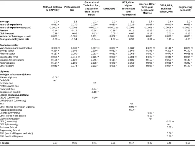
Because of the small number of observations for some diplomas, we pool some diplomas for the estimations. In case of pooled estimations, we identify the specific effect of a given diploma by a dummy. We use a particular methodology to decide which diplomas have to be pooled. The pooling is based on the proximity of diplomas regarding their situation in the labour market. In order to identify the proximity of diplomas we use a data analysis whose results are available on request. When the results of the data analysis are not sufficient, the pooling is based on the proximity of diplomas considering their higher education level. Finally, eight earning equations are estimated with six equations concerning higher education diplomas. The results of the estimates are shown in table 4.1.

23

Table 4.1. Estimation of earning equations by diploma

Intercept 2.2* 2.3* 2.2* 2.2* 2.1* 2.7* 2.6* 3.0*

Years of experience 0.012* 0.030* 0.020* 0.030* 0.026* 0.037* 0.040* 0.055*

Years of experience (square) -0.0001* -0.0005* -0.0001* -0.0002ns -0.0003* -0.0005* -0.0006* -0.0010*

Female -0.14* -0.12* -0.14* -0.16* -0.11* -0.13* -0.12* -0.16*

Civil Servant 0.18* 0.05** 0.13* 0.05** 0.07* 0.17* 0.01ns 0.13*

Number of hours (per month) -0.001* -0.001* -0.001* -0.002* -0.001* -0.003* -0.001* -0.003*

Young unemployment rate -0.08ns -1.54* -0.04ns 1.27ns 0.90* 0.04n s 0.19ns -1.85*

Economic sector

Manufactures and construction 0.003ns 0.030** 0.007ns 0.037** 0.033* 0.025n s 0.110* 0.026n s

Energy sector 0.254* 0.195* 0.230* 0.082* 0.166* 0.198* 0.201* 0.150*

Finance sector 0.117* 0.090* 0.063* 0.081* 0.063* 0.080* 0.071* 0.051n s

Services for firms -0.025* -0.018ns -0.015** 0.039* 0.004ns 0.029* * 0.041* 0.034***

Services for consumers -0.166* -0.122* -0.145* -0.114* -0.181* -0.152* -0.253* -0.140*

Administration -0.134* -0.100* -0.078* -0.070* -0.058* -0.095* -0.086* -0.242*

Other sectors -0.049* -0.074* -0.063* -0.055* -0.028* -0.086* -0.084* 0.120* Diploma

No higer education diploma

Without diploma -0.06*

CAP/BEP ref.

General Bac ref.

Professionnal Bac

Technical Bac -0.04*

Capacité en Droit (3) -0.10**

Higher education diploma

DEUG (University) 0.10*

DUT/DEUST (University)

BTS ref.

Other Higher Technician Diploma 0.00ns

Paramedical Diploma 0.17*

Licence (University) -0.08*

Other Three-Year degree 0.13*

Maîtrise (University) ref.

DEA (University) -0.01ns

DESS (University) ref.

Business School 0.07*

Engineering School

PhD (Medical Degree excluded) 0.06*

PhD (Medical Degree) 0.29* R-square 0.27 0.36 0.41 0.51 0.47 0.49 0.45 0.55 DESS, DEA, Business School, PhD Engineering School (1) Without diploma or CAP/BEP Professionnal Bac General and Technical Bac, Capacité en droit (3) and DEUG DUT/DEUST BTS, Other Higher Technicians and Paramedical Licence, Other three-year degree and Maîtrise

Source: French Labour Force Survey 2003-2005 (Insee)—authors’ calculation.

Note: (*) for 1% and (**) for 5% level of significance; (ns) for no significance. (1) The intercept presented here is not used in this form in the

simulations, see table 2.1 ; (2) Capacité en droit is a university law degree which does not imply passage of the Bac; it concerns almost 0.7% of the 1970 generation.

The individual residuals corresponding to the estimates are stocked and used during the simulation. Based on a random process, the microsimulation gives each simulated individual an observed residual depending on his diploma. During the dynamic simulation process, the residual is conserved until the individual leaves employment; when he finds a new job, a new residual is then randomly matched. Unfortunately, data on self-employment earnings are not available in the FLFS. In the simulation we decided to impute wages as a proxy of self-employment earnings.

24

Diagram 4.1. Wages in the GAMEO model

4.2. The socio-fiscal regime

The microsimulation takes into account the main features of the French socio-fiscal regime: the unemployment benefit, pensions and income tax. According to French social legislation, the calculation of workers’ rights to unemployment benefits and pensions is linked to gross wages, which are not available in the FLFS. We assume that the gross wages are a fixed share (120%) of net wages, which are available in the FLFS.

The regular unemployment benefit is simulated: the Allocation d’aide au retour à l’emploi (ARE). The entitlement and the amount of that benefit is legally linked to past wages and employment duration. In our simulation the amount of the allowance is calculated for the individuals who become unemployed on the legal basis.

25

The three main parts of the pension system are simulated. The basic pension is calculated based on the 25 best years, which are simulated. The differing complementary are also calculated. White-collar professionals (cadres) have a specific scheme. We assume that those with a five-year higher education degree or more are cadres. The complementary pensions are based on payroll taxes actually paid over the career. The civil servants’ regime is also simulated; it concerns those who have worked more than 41 years in the public sector; their pension is a fixed share of their last wage.

The French income tax is based not on individuals but on a particular definition of a household. Theoretically, the tax depends on the number of people (including children) in this ‘fiscal household’. In our simulation, we assume that the individual is single. This means that the macro revenues of income tax are overestimated as far as they do not take into account the wage cut (dépense fiscale) for family conditions (capacité contributive).

5. Modelling life expectation differentiated by education level

The existence of a correlation between education and life expectancy is well documented14 and confirmed for France15. However, the real impact of education on life expectancy is hardly apprehended, because of the correlation of education with some other variables (mainly the income) which may impact life expectancy. When one controls for the effect of these variables the impact of education tends to decrease but remains significant16. In this framework, our modelling strategy consists in introducing in GAMEO a mean life expectation for each individual corresponding to his education characteristics.

In France mortality tables by education level are not available. However Vallin and Meslé (2001) and Robert-Bobée (2006) give some cross-section mortality tables by socio-economic status. To estimate the mortality tables by diploma for the individual of a given generation we proceed in two steps. In a first hand, we estimate cross-section mortality tables by diploma for the 1991-1999 period—section 5.1. In a second hand, we define a method to forecast these tables for other periods—section 5.2.

14

For instance Kunst and Mackenbach (1994), Mackenbach et alii (2003, 2008).

15 _{Menvielle et alii (2007).}

16 _{See for instance Schnittker (2006), Cutler and Lleras-Muney (2006)}

26

5.1. Modelling survival functions

To model mortality differentials, we first compute a mortality table by diploma. We use mortality tables by age, gender and socio-economic status—currently available for France— and the French Labour Force Survey (FLFS) for this computation. Robert-Bobée and Monteil (2005) provided mortality rates for the 1991-1999’s period. In order to transform these tables, we apply the mortality rates by age, gender and socio-economic status for this period to the individuals in the FLFS 2003-2005. We then compute the average mortality rate by level of education in the FLFS sample. This sample is too small to produce highly disaggregated tables by level of education so we had to combine some diplomas. In the aggregation process, we choose to maintain as much as possible a differentiation by education type: for instance we differentiated the high school degrees according to their type—general versus specialized—, we differentiated the higher education diplomas according to their specificity —grandes

écoles versus University degree. Finally, we retain eleven diploma categories:

1- The individuals who do not have post-primary school diploma. 2-Those who have a professional middle-school degree (CAP,BEP). 3-Those who have a ‘general’ high school degree (General Baccalauréat).

4-Those who have a ‘specialized’ high school degree (Professional Baccalauréat Technical Baccalauréat) or who complete a particular Law University degree which is open to those who do not pass their high school degree (capacité en

droit).

5-Those who have a two years higher education degree (DEUG, DUT, BTS, High level technical degree).

6-Those who have a two years higher education degree in paramedical training. 7-Those who have a three years higher education degree.

8-Those who completed a four- years degree at University (maîtrise) or in a school. 9-Those who completed a master degree at University (research oriented or professional).

10-Engineering and Business Schools ’ master degree. 11-Those who have completed a PhD

27

The data on mortality rates by socio-economic status and the FLFS used do not correspond to the same period. The mortality tables concern the 1991-1999’s period, but they were applied to the FLFS 2003-2004. A computation based on the FLFS 1991-1999 was possible, but we choose to not use it because the available diploma variable for that period is not disaggregated enough for the analysis we intend to carry out. This mismatch in the periods might affect the mortality rates if the relative proportion of various socio-economic groups in the population has changed between 1991-1999 and 2003-2005. In order to assess the extend of this potential problem, we analyse the repartition of the population into the various socio-economic groups between 1999 and 2003, the last years of the two periods considered—the tables are available on request. We find that this repartition hasn’t changed significantly overall, although there are a few changes that introduce a small bias in our estimations. For example, between the two years, the proportion of individuals with a university degree that are in a high socio-economic status has slightly decreased, and at the same time the proportion of these individuals that are out of the workforce has slightly increased. Knowing that individuals in high SES have a lower mortality rate than those that are out the workforce, the observed trend will induce a slight overestimation of the mortality of the individuals with postsecondary education, compared to the real mortality rates by level of education between 1991-1999. In a similar manner we slightly underestimate the mortality of individuals with lower level diplomas. The consequence of this is that we might slightly underestimate mortality differentials by level of education.

The second step is to estimate the relationship between mortality by age and diploma. In order to do so, we estimate a function that differentiates the effect linked to the mean mortality of a generation (β) from an age effect (γand δ ) and an intercept (α ). We estimate the following equation for men and women separately:

where: e e α1 α2. α = + e e β1 β2. β = + 2 . . 1 log . 1 log a a M M M M e e a a e e a e a e α β +γ +δ       − + =       −

28 e e γ1 γ2. γ = + e e δ1 δ2. δ = +

and M stands for Mortality rate, s for sex, a for age, and e for level of education.

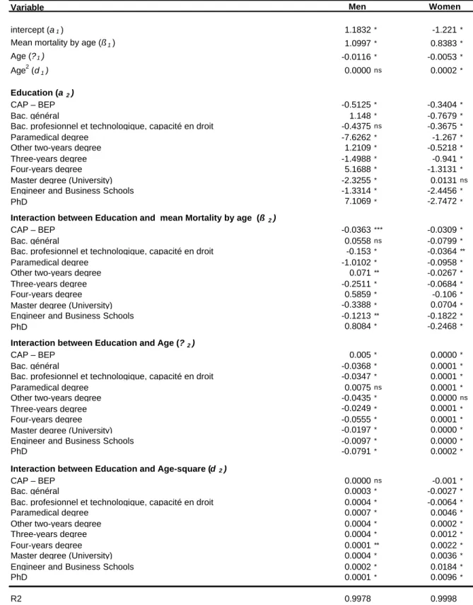
The interaction terms reflect the fact that the impact of the level of education on mortality is not due solely to a difference in the intercept -the coefficient a- of the mortality curves -i.e. a difference in value for each age-, but also to a difference in the slope –the coefficient b- of the curves -i.e. a difference in the evolution of mortality as age increases. This specification is inspired by Insee (1999), but we add interactions with age -and age squared- to reflect the fact that the impact of the level of education on mortality decreases towards the end of life. This specification is justified by Robert-Bobée et Cadot (2007)’s results: they show that although mortality differentials persist in old age, their magnitude decreases. We estimate equation 8 using on the one hand the mortality tables by level of diploma that we computed, and on the other hand the mortality tables by age and sex provided by Vallin and Meslé (2001). The results of our regression are reported in table 5.1.

This modelling enables the computation of survival functions. As expected, those with the highest levels of education have better survival rates. Consistent with the literature, mortality differentials are smaller for women.

29

Table 5.1. Regression of mortality by age on mortality by level of education Variable

intercept (a1) 1.1832* -1.221*

Mean mortality by age (ß1) 1.0997* 0.8383*

Age (?1) -0.0116* -0.0053*

Age2 (d1) 0.0000ns 0.0002*

Education (a 2)

CAP – BEP -0.5125* -0.3404*

Bac. général 1.148* -0.7679*

Bac. profesionnel et technologique, capacité en droit -0.4375ns -0.3675*

Paramedical degree -7.6262* -1.267*

Other two-years degree 1.2109* -0.5218*

Three-years degree -1.4988* -0.941*

Four-years degree 5.1688* -1.3131*

Master degree (University) -2.3255* 0.0131ns

Engineer and Business Schools -1.3314* -2.4456*

PhD 7.1069* -2.7472*

Interaction between Education and mean Mortality by age (ß ₂)

CAP – BEP -0.0363*** -0.0309*

Bac. général 0.0558ns -0.0799*

Bac. profesionnel et technologique, capacité en droit -0.153* -0.0364**

Paramedical degree -1.0102* -0.0958*

Other two-years degree 0.071** -0.0267*

Three-years degree -0.2511* -0.0684*

Four-years degree 0.5859* -0.106*

Master degree (University) -0.3388* 0.0704*

Engineer and Business Schools -0.1213** -0.1822*

PhD 0.8084* -0.2468*

Interaction between Education and Age (? 2)

CAP – BEP 0.005* 0.0000*

Bac. général -0.0368* 0.0001*

Bac. profesionnel et technologique, capacité en droit -0.0347* 0.0001*

Paramedical degree 0.0075ns 0.0001*

Other two-years degree -0.0435* 0.0000ns

Three-years degree -0.0249* 0.0001*

Four-years degree -0.0555* 0.0001*

Master degree (University) -0.0197* 0.0000*

Engineer and Business Schools -0.0097* 0.0000*

PhD -0.0791* 0.0002*

Interaction between Education and Age-square (d 2)

CAP – BEP 0.0000ns -0.001*

Bac. général 0.0003* -0.0027*

Bac. profesionnel et technologique, capacité en droit 0.0004* -0.0064*

Paramedical degree 0.0007* 0.0046*

Other two-years degree 0.0004* 0.0002*

Three-years degree 0.0004* 0.0012*

Four-years degree 0.0001** 0.0022*

Master degree (University) 0.0004* 0.0036*

Engineer and Business Schools 0.0002* 0.0184*

PhD 0.0001* 0.0096*

R2 0.9978 0.9998

Men Women

Source: FLFS 2003-2005 (Insee), Vallin and Meslé (2001), Robert-Bobée and Monteil (2005)-authors’

calculations.

Note: The category of reference for the education variable is « No Diploma ».

30

4.2. Forecasting survival functions

The previous sub-section showed how we estimate mortality differential by diploma at a given point of time. In this subsection, we explain the methodology of forecasting mortality rate for a given generation which by definition covers several points in time. To illustrate this issue, if one considers the 1970’s generation, one needs the differential in mortality rate in 2000, when the individuals are thirty17 ; for this, we can reasonably use the estimations previously presented (which is for the 2003-2004 period), but the mortality rate differential is also needed for each year of the period where an individual born in 1970 is still alive.

Mortality rates have been decreasing in France for the past two and half centuries (Pison 2005) and in order to model the average yearly decrease in mortality rate we need the mortality rates for two points in time. Unfortunately the only mortality forecasts available are of mortality by age and gender only –see Vallin and Meslé (2001). There are no mortality forecasts for 2049 by level of education, so we made the hypothesis that the evolution of mortality rates over time is the same regardless of the level of education. We therefore applied the average yearly decrease in mortality by age and gender only to the mortality rates by education level. This hypothesis is conservative and does not correspond to results available on the evolution of mortality rate by education level in France (Menvielle et al 2007). This conservative hypothesis is however the one that is the most consistent with our methodology. In the estimation of salaries in the microsimulation model, we do not include a change in the wage differential by level/type of diploma. Similarly we do not model any other changes over time (such as changes in access to health care for example) that could explain the evolution of the mortality differential. It is therefore only coherent that we would choose the conservative hypothesis under which the mortality differential by level of education remains constant over time in our model.

This extrapolation assumes that mortality decreases in a linear manner over time. This assumption seems reasonable given the fact that the evolution of mortality rates in France has so far been linear, as the available data shows (Vallin and Meslé 2001).

17

We do not consider mortality differentials before 30 years because the full impact of education differentials on mortality are not likely to be visible before that age. In addition, individuals who decide to pursue studies that last long (such as medicine or a doctorate) are not likely to enter the workforce before they are around 30 years old.

31

To forecast the mortality rate differential throughout the years, we use mortality rates in 1991-1999 and we extrapolate them from the mid point of the 1991-1991-1999 period—i.e. 1995-— forward to the desired year, as follows.

where Mae (n) is the mortality rate by age and level of education for year n.

We first compute the difference between the log of mortality rates at two periods—here in 1995 and in 2049—and then divide this value by the number of years separating the two periods—here 54—, to obtain the average yearly decrease in the log of mortality. This yearly increase is then multiplied by the number of years between the year of interest—here it is n— and the starting year—here 1995—, and added to the log of the mortality rate in the starting year -here 1995.

In the ageing process of GAMEO there is not ‘real killing’ of individuals: each individual trajectory is simulated from age 16 to age 100. However, there is a specific weight of the individual for every year. It is calculated by correcting the individual weight of the former year by the mortality rate at this given age.

5. Conclusion

With the GAMEO model it is possible to simulate the distribution of the chronicles of income for a given generation. Until now, the model has been mainly used to simulate the trajectories of the generation of the individuals born in 1970 and to discuss French higher education policy. This output joined with a set of hypothesis, consisting mainly in defining the opportunity cost of one more year of education, enables to calculate individual indicators like internal rate of return to education and to decompose them: Courtioux and Houeto (2009) propose a risk analysis of return to education and discuss the implicit monetary incentive framework of complete a given diploma; Courtioux (2008, 2009) analyses the impact of the implementation of an income contingent loan for higher education18 on the individual returns to education. This output can also produces macro indicators: Courtioux (2008, 2009)

18 _{For a general presentation of income contingent loan see Chapman (2006).}

( )

(

)

(

) (

)

32

evaluates the revenues of different income contingent loan schemes as well as the progressive development of these revenues.

However, to produce more complete policy evaluations the GAMEO model has to be further developed in several ways. An important challenge is to introduce the simulation of family formation and its implications for income tax and other elements of the French socio- fiscal regime. This part is important to go further than a simple risk analysis and to produce a more precise insight of the macro implications of the policies analyzed. Another aspect is to strengthen the estimation of mortality rate by diploma, which could be done by an access to some demographic data like the Echantillon Démographique Permanent (Insee).

More generally, the model is based on the structure of the ‘new’ annual French Labour Force Survey; the availability of new data will enables us to produces more precise estimations of earning equations and transition equations for the forthcoming versions of the GAMEO model.

References

Albouy V. Wanecq T. (2003), “Les inégalités sociales d’accès aux grandes écoles”, Economie

et Statistique, n°361, p.27-47.

Chapman B. (2006a), “Income Contingent Loans for Higher Education: International Reforms”, in Hannushek E.A., Welch F. (eds), Handbook of the Economics of Education, Volume 2 , Elsevier, p. 1435-1503.

Commission of the European Communities (2005), Progress towards the Lisbon objectives in

education and training, 2005 Report, Commission staff working paper, SEC (2005) 419,

Brussels.

Courtioux P. (2008), “How Income Contingent Loan could affect Returns to Higher Education: a Microsimulation of the French Case”, Society for Advancement of

Socio-Economics’ Annual Meeting, July 21-23, San Jose, Costa Rica.

Courtioux P. (2009), “Peut-on financer l’éducation du supérieur de manière plus équitable ?”,

position paper, EDHEC Business School, January.

Courtioux P., Houeto D. (2009), “L’analyse socio-économique des cheminements longs : l’apport de la microsimulation dynamique dans le champ de l’éducatio n”, XVIèmes Journées

d’Etude « Les données longitudinales dans l’analyse du marché du travail », CEREQ-Centre

d’économie de la Sorbonne, June 4-5, Paris, France.

Harding A. (1993), Lifetime Income Distribution and Redistribution: Applications of a

Microsimulation Model, Contribution to economic Analysis series, Amsterdam,

North-Holland.

33

Heckman J., Lochner L., Todd P. (2006), “Earning Functions, Rates of Return and Treatment Effects: The Mincer equation and beyond”, in Hannushek Eric A., Welch Finis (eds),

Handbook of the Economics of Education, Volume 1 , Elsevier, p. 307-458.

Cutler D., Lleras-Muney A. (2006), “Education and Health: Evaluating theories and evidence”, NBER working paper, n° 12352.

Gazier B., Schmid G. (eds) (2002), The dynamic of Full Employment. Social Integration by

Transitional Labour Markets, Edward Elgar, Cheltenham.

Insee (1999), « Le modèle de microsimulation Destinie », document de travail Insee, division redistribution et politique sociale.

Kunst A., Mackenbach J. (1994), “The Size of Mortality Differnces Associated with Educational Level in Nine Industrialised Countries”, American Journal of Public Health, 84 (6), p. 932-937.

Mackenbach J.P., Bos V., Andersen O., Cardano M., Costa G., Harding S., Reid A., Hemström Ö., Valkonen T., Kunst E.A. (2003) « Widening socioeconomic inequalities in mortality in six Western European Countries”, International Journal of Epidemiology, 32 (5), p.380-387.

Mackenbach J.P., Stirbu I., Roskam R. A.-J., Schaap M.M., Menvielle G., Leinsalu M., Kunst E.A. (2008), « Socioeconomic Inequalities in Health in 22 European countries », The New

England Journal of Medicine, 358, p.2468-2481.

Maurice M., Sellier F., Silvestre J.-J. (1982), Politique d’éducation et organisation

industrielle en France et en Allemagne. Essai d’analyse sociétale, Presse Universitaires de

France.

Menvielle G., Chastang J.-F., Luce D., Leclerc A., (2007), « Evolution temporelle des inégalités sociales de mortalité en France entre 1968 et 1996. Etéude en fonction du niveau d’études par cause de décès », Revue d’Epidémiologie et de Santé Publique, 55, p.97-105. Mincer J. (1974), Schooling, Experience and Earnings, Columbia University Press, New York.

Mitton L., Sutherland H. Weeks M. (2000), Microsimulation Modelling for Policy Analysis.

Challenges and Innovations, Cambridge University Press.

Pison G. (2005), « France 2004 : l’espérance de vie franchit le seuil des 80 ans », Population

et Sociétés, n° 410.

Robert-Bobée I. (2006), “Projection de population 2005-2050 pour la France métropolitaine”, Working Paper, Insee, Methodes et Résultats, n° F0603.

Robert-Bobée I. (2006), “Projection de population 2005-2050 pour la France métropolitaine”, Document de travail Insee, Méthode et résultats, n° F0603.

Robert-Bobée I., Cadot O. (2005), “Mortalité aux grands âges : encore des écarts selon le diplôme et la catégorie sociale”, Insee Première, n° 1122.

Robert-Bobée I., Monteil C. (2005), “Quelles évolutions des différentiels sociaux de mortalité pour les femmes et les hommes ? Tables de mortalité par catégorie sociale en 1975, 1982 et 1990 et indicateurs standardisés de mortalité en 1975, 1982, 1990 et 1999”, Document de travail Insee, n° F0506.

34

Schmid G. (2006), “Sharing Risk Management through Transitional Labour Markets”,

Socio-economic Review, 4, p.1-33.

Schnittker J. (2004), “Education and the Changing Shape of the Income Gradient in Heath”,

Journal of Health and Social Behavior, 45, p.286-305.

Vallin J., Meslé F. (2001), Tables de mortalité françaises pour les XIXe et XXè siècles et

projections pour le XXè siècle, INED, Paris, 102p.

Zuber S., (2004), “Evolution de la concentration de la dépense publique d’éducation en France 1900-2000”, Education et formation, n° 70, p. 97-108.