HAL Id: hal-01092485
https://hal.archives-ouvertes.fr/hal-01092485
Submitted on 21 Feb 2017HAL is a multi-disciplinary open access archive for the deposit and dissemination of sci-entific research documents, whether they are pub-lished or not. The documents may come from teaching and research institutions in France or abroad, or from public or private research centers.
L’archive ouverte pluridisciplinaire HAL, est destinée au dépôt et à la diffusion de documents scientifiques de niveau recherche, publiés ou non, émanant des établissements d’enseignement et de recherche français ou étrangers, des laboratoires publics ou privés.
Distributed under a Creative Commons Attribution - NonCommercial - NoDerivatives| 4.0 International License
A beam to 3D model switch for rotor dynamics
applications
Mikhael Tannous, Patrice Cartraud, David Dureisseix, Mohamed Torkhani
To cite this version:
Mikhael Tannous, Patrice Cartraud, David Dureisseix, Mohamed Torkhani. A beam to 3D model switch for rotor dynamics applications. Engineering Structures, Elsevier, 2015, 84, pp.54-66. �10.1016/j.engstruct.2014.11.020�. �hal-01092485�
A beam to 3D model switch for rotor dynamics applications
Mikhael Tannous a, Patrice Cartraud a, David Dureisseix b, Mohamed Torkhani c
a GéM, Ecole Centrale de Nantes, France
b Université de Lyon, LaMCos, INSA de Lyon, CNRS UMR 5259, France
c LaMSID UMR EDF-CNRS-CEA 2832, EDF R&D, F-92141 Clamart Cedex, France
Abstract
A typical accidental slowing down of a turbine presents a rotor–stator contact that may be limited to a small interval of the whole simulation period. Such engineering problems involving slender structures with local or non-linear phenomena restricted in time require a 3D model for a better understanding of the local or non-linear phenomena, whereas a simplified beam model can be sufficient for simulating the linear phenomena occurring for a long period of time.
This paper proposes a strategy that enables to switch from a beam model to a 3D model during a transient rotor dynamics analysis, and thus, allows to reduce the computational cost while preserving a good accuracy.
The simulation starts with a beam model, and at the switch instant ts, the 3D solution is initialized as the
sum of a displacement corresponding to the classical Timoshenko kinematics assumption and a 3D correction that accounts, for instance, for cross-section deformation. This is performed on three consecutive time steps (the switch instant, the previous and the following steps), thus allowing to make velocity and acceleration corrections.
The method is proved to be energetically sound and is validated through comparisons with a reference solution corresponding to the 3D model solution computed during all the simulation.
This is a preprint of an article published in its final form as: Mikhael Tannous, Patrice Cartraud, David Dureisseix, Mohamed Torkhani, A beam to 3D model switch for rotor dynamics applications, Engineering
Structures 84:54-66, 2015. doi: 10.1016/j.engstruct.2014.11.020. 2014 Elsevier Ltd.
Keywords: Rotor dynamics; Finite elements; Switch; Energy consistency
1. Introduction
Many industrial problems in transient dynamics, such as the simulation of turbine accidents, require a 3D model in order to accurately account for local effects such as rubbing, that occur along a small period of time. However, a 3D model for the entire structure used during the whole simulation will result in an unaffordable computational cost even on the best nowadays computational machines and softwares. We, therefore, present a method that can reduce dramatically the computational cost, for problems where the 3D non-linearities are restricted in space and time.
To solve problems for which non-linearities are restricted in time, one can use a time integration scheme switching technique. In fact, when non-linear phenomena occur, such as contact interactions, small time steps are needed to ensure an accurate modeling of the physical phenomenon. In such cases, an explicit integration method is well suited to reduce the computational cost. However, for the complementary part of the problem which is linear, an implicit method presents the advantage of unconditional stability, thus making it possible to use larger time steps. An algorithm that enables one to switch automatically between explicit and implicit integration scheme thus significantly reduces the computational cost. Narasimhan and
Lovell [1] and Jung and Yang [2] proposed, respectively, an explicit to implicit and implicit to explicit time integration switches for sheet metal forming applications. Explicit to implicit and implicit to explicit switches were used in Lo et al [3] for improving the computational cost of the simulation of impact crash problems. In Noels et al [4,5], the authors developed automatic criteria for time integration scheme switching techniques and applied it for non-linear structural dynamics. This technique has also been applied in Noels et al [6,7] to metal forming simulation and in Noels et al [8] for a blade/casing interaction simulation. These explicit/implicit and implicit/explicit switches have been recently implemented in the industrial finite element code Code_Aster based on the research work of Mahjoubi et al [9] when implicit and explicit domains are not located in the same area, and a domain decomposition-like method is used to couple them.
For phenomena that are restricted in space, i.e. to a small part of the computational domain, a wide range of methods has been developed. These approaches are always in progress and can be divided into exact (or direct) methods and iterative ones. The most popular exact approaches are the static condensation techniques and the exact structural reanalysis methods, such as used in Hirai [10], Hirai et al [11]. Adaptive meshing techniques can be used for a local refinement of a 3D model, see for example Plaza et al [12]. Volume patches such as Arlequin enable to superpose two different domains, e.g. a beam model and a 3D model. Applications examples can be found in Ben Dhia [13], Ben Dhia and Rateau [14], Cottereau et al [15], Ghanem et al [16]. Beam to 3D connections or shell to 3D connections, enable to account accurately for local 3D phenomena, while the rest of the model is less computationally expensive thanks to the beam or shell elements. Many applications in the literature exist such as the mixed beam-3D model used by Kettil and Wiberg [17] for the simulation of a bridge deformation.
The iterative domain decomposition methods can be divided into overlapping and non-overlapping domain decomposition methods. Multi-scale methods with patch are overlapping domain decomposition methods that enable to have a local zoom on the domain; the superposition methods consist in making a local correction on a global domain, such as the finite element patches Lions and Pironneau [18], Glowinski et al [19] and the harmonic patches He et al [20].
Non-overlapping domain decomposition methods can be classified into three main categories: the primal approaches Mandel [21], the dual approaches (FETI method) that appeared in the early 1990s Farhat and Roux [22], and the hybrid or mixed approaches such as FETI-DP, which is an improved version of the FETI method, that combines the advantages of the dual and primal approaches Farhat et al [23]. FETI has also a multi-scale version used in Mobasher Amini et al [24] and Mobasher Amini et al [25] for the computation of ship structures where windows are some centimeters wide, whereas the structure of the ship is hundreds of meters long. For similar applications we also find the micro–macro approaches, see Ladevèze et al [26].
Regarding local non-linear phenomena, FETI was enhanced to deal with large number of subdomains and can take geometric non-linearities into account Farhat et al [27], and was adapted for contact problems in Avery et al [28], Avery and Farhat [29], Dureisseix and Farhat [30]. In Alart et al [31] we find an adapted Schwarz method for frictional contact problems. In Gendre et al [32,33], the authors developed an algorithm that enables to replace the global mesh by a finely meshed local zone, in order to take local non-linear effects into consideration with low computational effort. The use of beam to 3D connections or shell to 3D connections can also be useful for non-linear local phenomena. In Andrieux and Varé [34], a beam to 3D connection was successfully used for a study of local cracking in a turbine rotor.
Turbine accident problems present non-linear phenomena that are restricted both in time and space. For non-linearities restricted in space, i.e. for the time period where no contact interactions take place, a beam model is sufficient to model the slowing down of the turbine as done in Roques et al [35]. However, in this reference the authors also used the beam model for local rotor stator interactions modeling. To be able to accurately account for the local rotor stator interactions, a 3D local model is mandatory. The remaining parts of the turbine do not exhibit non-linear local phenomena and can be modeled by beam elements. Therefore, a model that mixes beam and 3D elements, connected with appropriate constraints, can be very
useful to model non-linearities restricted in space. This approach has been proposed in Tannous et al [36,37] for transient dynamic applications excluding overall rotations, based on the PhD of Tannous [38].
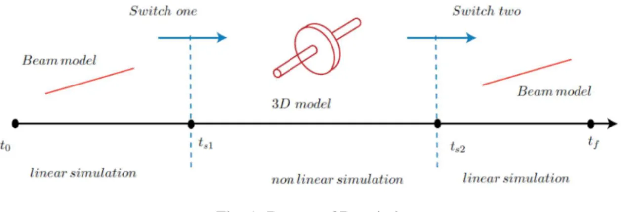
Therefore, this research article goes one step further and addresses the issue of reducing the computational cost for non-linear phenomena restricted in time and for rotor dynamic applications. The simulation starts at t = t0 with a beam model for a linear simulation, and switches at t = ts1 to a 3D model
when a non-linear phenomenon is to take place. The simulation switches back at t = ts2 to the beam model
for of the rest of the simulation that ends at tf, if no more non-linear phenomenon is present as illustrated in
Fig. 1. This strategy, called the switch method, presents several difficulties when applied to rotor dynamics applications in comparison with a switch method for transient dynamic problems excluding overall rotations. In fact, the beam and the 3D solutions of the same rotor dynamics problem are slightly phase shifted. This make the switch method a challenging task since the solutions shift leads to a non-negligible difference between the 3D and the beam solutions at the switch instant. This issue as well as other difficulties are addressed in the scope of this paper.
Fig. 1. Beam to 3D switch.
This paper presents a beam to 3D model switch. The 3D to beam model switch is not the subject of this research work. The switch method is independent from the switch instant choice. This latter is chosen arbitrarily in this research article for sake of simplicity, since the main objective of this article is to present the switch from a methodological and academic point of view such a way the method works whatever the switch instant is. However, the switch has to be performed in the linear stage preceding the appearance of non-linear phenomena. This represents the main switching criteria for all type of applications. For a rotor– stator contact problem, when a rotor to stator contact is detected on the beam model at a given instant tc, the
switch instant is calculated by ts = tc − n ∆t, where ∆t is the time step and n is a safety factor that enables to
perform the switch sufficiently far from any non-linearity. Moreover, since this paper is focused on the switch process, linear problems are considered.
2. Unbalanced rotor dynamics modeling
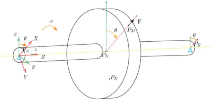
The loss of a terminal blade of a turbine creates an unbalance of mass M at a distance d from the axis of rotation, which rotating at an angular velocity ω. This produces an unbalance force F = M d ω2 applied where the mass breakdown took place. We are interested in the dynamic response of such an unbalanced rotor.
Different modeling techniques enable to describe the dynamic response of the unbalanced rotor. Beam based models, such as described in Section 2.1, are simple and efficient models. They are of satisfactory precision if no local phenomena are observed. If local phenomena occur, such as a rotor to stator
contact/friction interactions, 3D elements are required to accurately capture these effects. Such a modeling technique is detailed in Section 2.2 and is computationally expensive.
Note that in the following, we present the beam modeling as well as the 3D modeling of an unbalanced rotor. The finite element software that we are using in the scope of this research paper is Code_Aster developed by the Research and Development section of EDF [39]. Code_Aster proposes a beam modeling of an unbalanced rotor in the Galilean frame, whereas the 3D modeling of the unbalanced 3D rotor, taking into account the gyroscopic effects of the 3D elements recently developed in the scope of the PhD thesis of Ghanem [40], takes place in the rotating frame. In this article, we therefore use for rotor dynamics modeling, the rotating frame for the 3D model, and the Galilean frame for the beam model. The gyroscopic matrix of the 3D elements is dependent on the rotation velocity. The rotor dynamic problem is non-linear if the rotation velocity is an unknown of the dynamic problem. Code_Aster deals with rotor dynamic problems in which the rotating velocity is given. We, therefore, for the following application examples deal with a constant and given rotating velocity; though the switching technique itself is fully applicable to rotor dynamic problems for which the rotating speed is an unknown.
2.1. Beam modeling of a rotor subjected to unbalance loading
Let us consider a rotor as schematically shown in Fig. 2. An unbalance load F = M d ω2 is triggered by the loss of a mass M located at point PM at a distance d from the axis of rotation of the rotor turning with an
angular speed ω.
The equivalent beam model of the rotor is show in Fig. 3, with a discrete rigid disk. In other terms, the inertia and mass properties of the disk are affected to the beam node that corresponds to the disk position, namely point PN in Fig. 3. The disk deformation is not taken into account in such a simplified model.
The fundamental dynamic equation of a beam model subjected to a rotation unbalance Fb in the Galilean
frame Rg, where Ubg is the beam displacement vector, reads:
(1)
Mb, Ab and Kb represent respectively the mass, damping and stiffness matrices of the beam model. Gb(ω) is
the gyroscopic matrix. This later is a function of the rotating velocity ω.
In these conditions and in the frame Rg, the unbalance Fb has two components: one along to the x-axis
named Fx =M d ω2 cos(ωt), and the other along the y-axis direction Fy =M d ω2 sin(ωt).
Fig. 3. Beam model of the rotor.
2.2. 3D modeling of a rotor subjected to unbalance loading
The fundamental equation of motion of a 3D rotor model, as the one shown in Fig. 2, subjected to unbalance, in the rotating frame R at an angular velocity ω, reads:
(2)
, , and are respectively the displacements, velocities and accelerations of the 3D model. M3D,
G3D(ω), A3D and K3D are respectively the mass, gyroscopic, damping and stiffness matrices of the 3D
model. is the unbalance force written in R. has a fixed direction in R and a module F3D = M d ω2.
Note that in the rotating frame R, the gyroscopic matrix G3D(ω) is the matrix that takes into account the
gyroscopic effects of the 3D elements as well as the Coriolis and dragging forces, Lalanne and Ferraris [41].
3. Beam to 3D model switching
Since the beam modeling of the unbalanced rotor is described in the Galilean frame and the 3D modeling in the rotating one, switching for one model to another supposes firstly to use the same frame for both the models. We, therefore, need to make a frame transition for the beam solution (from the Galilean to the rotating frame), before switching to the 3D model.
3.1. Frame transfer matrix
We consider that the rotation of the rotor is occurring around its z-axis as illustrated in Figs. 2 and 3. The beam displacements , velocities and accelerations written in the Galilean reference Rg are
transferred to the rotation frame R and are denoted respectively , and , by using a frame transfer matrix Qb. The frame transition can be summarized by the following expressions:
(3)
2
cos −sin 0 sin cos 0 0 0 1 0 0 0 0 0 0 0 0 0 0 0 0 0 0 0 0 0 0 cos −sin 0 sin cos 0 0 0 1 (4)
where θ represents the angle of the rotation of the rotor from its initial position.
3.2. Basics of the switch
A beam model simulation starting at t = 0 is to be switched for a 3D model simulation at t = ts. Starting
with the 3D model at t = ts requires the collection of the beam model solution at ts and transforming this
solution to have a suitable 3D model initialization at the same instant. The construction of the 3D solution at
t = ts relies on the decomposition of the solution in three main components:
1. A rigid body motion (rotation). This part of the solution is already decoupled from the two other parts of the solution, since in Code_Aster the rotation velocity is given and the 3D solution is written in the rotating frame.
2. A beam solution corresponding to rigid body cross-sections (Timoshenko kinematical assumption), . A projector matrix P, introduced in Tannous et al [36] and recalled in Appendix A, can be defined to transform the beam displacement vector into a 3D rigid body displacement per beam section P . Since the beam and the 3D solution are expressed in different frames, the beam solution is first transformed to the rotating frame by Eq. (4), to give P .
3. A 3D correction denoted with , expressed in the rotating frame. The 3D solution at t = ts, in the rotating frame, reads:
(5)
Therefore, 3D dynamics Eq. (2) leads to:
(6)
, and are three corrective terms. However, since we have one equation with three unknowns, additional assumptions should be made.
3.2.1. First strategy
In a first step, we neglect the velocities and accelerations corrections ( and ) and compute the displacements corrections at t = ts in a static computational step:
− − − (7)
The computations of and can be done in the same way as , using Eq. (4). The 3D model can therefore be initialized at t = ts with:
This strategy is quite cheap from a computational cost point of view, but the strong assumption consists in neglecting and . At a consequence, they initiate, at the switch instant, a transient stage with high frequency oscillations, mostly on the accelerations of the 3D solution. To stabilize the solution after switching, and as proposed in Tannous et al [36], one can filter these high frequency oscillations by introducing a numerical damping in the time integration scheme (HHT integration scheme Hilber et al [42] for example), or make velocities and accelerations corrections (triple static switch procedure also discussed in Tannous et al [36]). This later method, proved to be efficient, eliminates completely the transient stage and provides a stable 3D switch solution. It is briefly presented in the following and is used in all the application examples of this article.
3.2.2. Second strategy
The second strategy, i.e. the triple static switch, consists on making three static switches by solving Eq. (7) at the switch instant ts, one time preceding ts and denoted ts−1 and at one time step following ts and
denoted ts+1. The velocities at t = ts will be computed according to the finite difference formula:
∆ (9)
The accelerations are computed in order to preserve the dynamic equation of the 3D model at ts, and thus
at ts is the solution of:
− − (10)
where is computed with Eq. (5), and is computed with Eq. (9).
If an implicit time integration scheme is used, e.g. one of Newmark time integration schemes family, then the accelerations will automatically be computed by the finite element software such a way they respect Eq. (10) as indicated by Géradin and Rixen [43].
3.3. Energy consistency of the switch
The precision of the switch is checked by comparing the switch solution with a 3D reference solution computed along the whole simulation period. Another method to check the validity and the robustness of the switch is to check its energy consistency. This is a procedure widely used in the literature. Noels et al [5,7] used this procedure to demonstrate the stability of an implicit/explicit time integration scheme switch method.
We consider a mechanical system rotating at an angular speed ω around an axis with a corresponding inertia I. In the rotating frame, F is the external load, U is the displacement vector, M and K are the mass and stiffness matrices. The kinetic energy can then be written as the sum of two components. The first component is related to the rotating inertia, namely, Wcr = ½ Iω2, and the second component is related to the
deformation of rotor Wcd = ½ .
The deformation energy reads:
(11)
(12)
Without dissipative sources, the kinetic energy theorem leads to:
(13)
where cst is a constant that depends on the problem being solved. If the external force is constant, one gets a constant energy balance:
− (14)
In our study case, the unbalance is a constant (it is a function of time for a short period before it reaches its given value, and the switch takes at an instant at which the unbalance is constant). Therefore, the energy consistency (i.e. the fact that the switch does not remove nor insert energy in the 3D solution after switching) can be checked by computing the total energy Wt of the 3D solution after switching, and
verifying that this later is constant and is close to the total energy of the 3D reference solution.
4. Application example on rotor dynamics
Let us consider a 3D rotor model, as the one shown in Fig. 2, made up of a steel material with a density ρ = 7800 kg/m3, a Young modulus E = 2.1 1011 N/m2 and a Poisson ratio ν = 0.3.
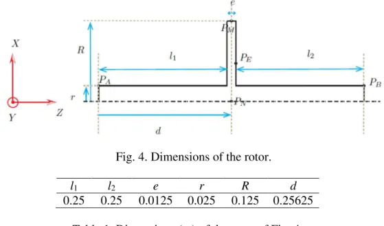
The half cross-section of the rotor is presented in Fig. 4. Table 1 gives the rotor dimensions.
Fig. 4. Dimensions of the rotor.
l1 l2 e r R d
0.25 0.25 0.0125 0.025 0.125 0.25625
Table 1. Dimensions (m) of the rotor of Fig. 4.
The rotor disk itself is modeled as a rigid part with a young modulus a hundred times higher than that of the rotor. The 3D rotor is meshed with quadratic elements and contains 1883 nodes with 3 degrees of freedom (dof) each, while its equivalent beam model with Hermite elements contains 43 nodes with 6 dof each.
In the following example, the rotor is pinned at its two extremities and is rotating at an angular velocity ω = 300 rpm and is subjected to a 1 kg unbalance at point PM as illustrated in Fig. 2. The studied time
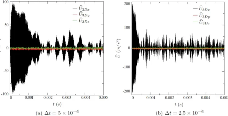
evolution spreads on 0.5 s, and is solved by the Newmark implicit mean acceleration scheme with 8000 time steps (∆t = 6.25 10 5 s). Note that applying the unbalance abruptly (at the first time step) will generate high frequency oscillations in the accelerations and velocities. This fact is illustrated in Fig. 5: dividing the time step by two, leads to a doubled acceleration.
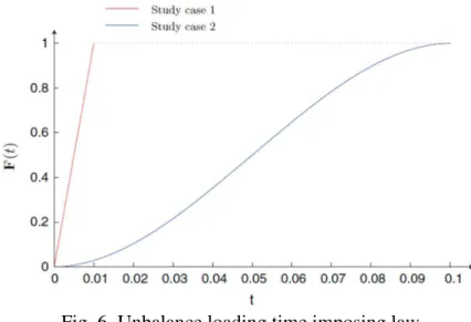
To address this issue, the unbalance is applied according to a given progressive time law. The rotor excitation will depend on this law1 but the switch method itself can manage all loading conditions. Fig. 6
shows two different unbalance laws. In the first, the unbalance F(t) is applied linearly during 0.01 s, and is kept constant afterwards. In the second, F(t) follows a more progressive evolution law, with null derivatives at t = 0 and at t = tm, instant at which the unbalance reaches its stable constant value. The switch instant is
ts = 0:25 s. After switching, the 3D solution is compared to a 3D reference solution computed along the
whole simulation period (0.5 s).
Fig. 5. Influence of the size of the time step if the unbalance is applied abruptly at the first time step.
1 Imposing the unbalance according to a given law has the effect of not generating numerical high frequency oscillations.
However, it may excite some high eigen-frequencies of the rotor, since such loading functions include a large series of high frequencies, even though the loading is smooth.
Fig. 6. Unbalance loading time imposing law.
We first present an application example for the first unbalance loading law, and for a 300 rpm rotating velocity.
Fig. 7 shows the displacements of point PN along the x-axis in the rotating frame (see Fig. 2)). The 3D
solution after switching is compared to the 3D reference solution.
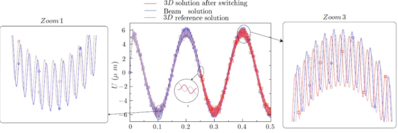
The results in Fig. 7 are transformed to the Galilean frame, and the displacements of point PN of the beam
model in its Galilean frame are added, thus resulting in Fig. 8.
We can note the presence of two vibration frequencies, the first one is that of the global rotation of the rotor. The second one is a modulation and represents the vibration of the rotor around its stable deflection posture (while rotating). This later is excited by the unbalance law, and is a physical response of the rotor. A Fast Fourier Transform (FFT) of this modulation shows a frequency close to 256 Hz, which is an eigen-frequency of the rotor2.As seen in Zoom 1 of Fig. 8, a shift exists between the 3D reference solution and the beam solution. This shift, that also can be seen on Figs. 7 and 9, is due a slight difference (around 1 %) between the eigen-frequencies of the beam and the 3D models, which in turn leads to a shift between the beam and the 3D solutions and not to the switch method. Having an enough slender beam and refining the 3D mesh model contributes to reducing this difference.
For the displacements results, the shift is noticed on the modulations (second eigen-frequency and not the first), but the evolutions of the two solutions are very similar and present very close amplitudes.
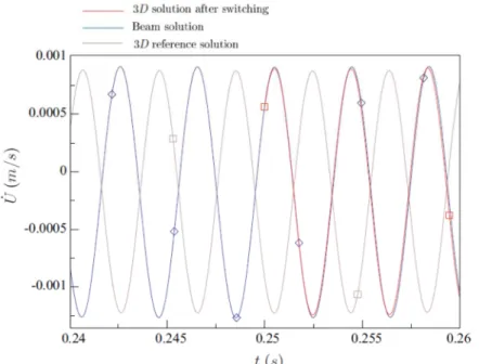
For the velocities and accelerations, this shift can be seen on the first eigen-frequency. Though at the switch instant, the beam at the 3D reference solutions may have anti-phase velocities and accelerations (Figs. 10 and 11), the amplitudes are very similar. In the following, and for a better clarity of the figures, the results are shown for t ∈ [0.24 s, 0.26 s]. Note that the same conclusions are also obtained on a point that does not belong to the neutral fiber of the rotor, such as point PM on which the unbalance force is applied
and for which the velocities and accelerations results are presented in Fig. 9.
2 The first three natural frequencies of the 3D rotor model are 255.597 Hz, 255.772 Hz and 374.534 Hz. Those of the beam rotor
Fig. 7. Displacements results along the x-axis of point PN (rotating frame).
Fig. 9. Velocities and accelerations results along the x-axis of point PM (rotating frame)
The 3D switch solution at t = ts is constructed from a beam solution ( ) at which a 3D correction
( ) is added. This implies that the 3D switch solution has the same deflection as the beam model at the switch instant. The 3D correction is mainly a cross-section deformation and cannot adjust the shift between the beam and the 3D solutions. Therefore, after switching, the 3D switch solution ‘‘clings’’ on the beam solution and has the same eigen-frequencies as the 3D reference solution. Thus, the shift is never compensated as shown on the displacements results in Fig. 8 as well as on the velocities (Fig. 10) and acceleration (Fig. 11) results. This is inevitable since it is not possible to have identical beam and 3D solutions behaviors3.
3 The same conclusions and quality of the results shown in Fig. 8 is also obtained on the y-axis direction and on each point
In spite of the phase shift between the beam solution and the 3D solution, the switch enables one to have a very good approximation of the 3D reference solution. The behavior of the 3D switch solution and the 3D reference solution is almost the same if the phase shift is isolated (same natural frequencies, amplitudes, etc.). No perturbations (high frequency oscillations, divergences, etc.) exist in the 3D switch solution. The switch allows to save computational cost while preserving a good accuracy.
Analyzing the energy consistency of the switch confirms the robustness of this later: no parasite energy is inserted nor removed from the solution at the switch instant.
Fig. 10. Velocities results along x-axis of point PN (Galilean frame).
Fig. 11. Accelerations results along x-axis of point PN (Galilean reference).
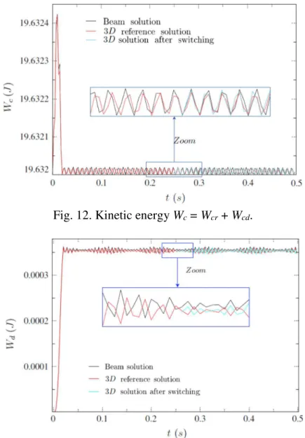
Figs. 12 and 13 present respectively the kinetic and deformation energies of the beam model, the 3D reference model and the 3D switch model. It must first be noted that the values of the kinetic, deformation and total energies are computed each 50 time step only. This is why the curves of energy are not ‘‘smooth’’.
The values of the kinetic and deformation energies of the 3D switch model are coherent with those of the 3D reference solution.
No energy disturbance occurs on the kinetic, deformation and total energy values at the switch instant. As previously explained in Section 3.3, the kinetic energy has two components: the first is related to the rotation of the rotor around its main axis and has a value of Wcr = ½ Iω2 = 19.632 J in our case, and the
second is related to the vibrational movement of the rotor (Wcd) and has a much lower main value. Wcr is
constant because the rotational velocity is constant, and Wcd oscillates. The switch does not disturb any of
the two kinetic energy components.
Fig. 12. Kinetic energy Wc = Wcr + Wcd.
Fig. 13. Deformation energy Wd.
Fig. 13 shows the deformation energy of the beam model, 3D reference model and the 3D switch model. We can notice that the nominal deflection of the rotor is established during the unbalance loading phase t ∈ [0, tm]. After this phase, the rotor vibrates around its stable equilibrium position. Thus, his strain energy
oscillates around a constant value. After switching, the value of the strain energy of the 3D switch model is consistent with that of the beam model and the 3D reference model, and no oscillations are found.
Fig. 14 shows the total energy, computed according to Eq. (14), of the beam, 3D reference and 3D switch models. Once the unbalance reaches its constant value (at 0.01 s in our case), the total energy is a constant
and that is obviously seen in Fig. 14. The 3D reference model and the 3D switch models have almost the same total energy. The switch does not insert nor remove energy from the system.
In the following, another application example is shown. The same physical and numerical conditions of the previous example are maintained in this following example, except the rotational velocity. The unbalance is applied according to the loading law of study case one of Fig. 6. The rotational velocity is increased to 1500 rpm, in order to show the robustness of the switch on another study case, and a higher rotational velocity. Results are shown on point PN along the x-axis direction. Note that the same conclusions
are obtained along the y-axis direction and on other points belonging to the rotor. Fig. 15 shows the displacements results in the rotating frame.
Fig. 14. Total energy Wt = Wc + Wd.
Fig. 15. Zoom on the displacements results at the switch instant for ω = 1500 rpm (rotating frame).
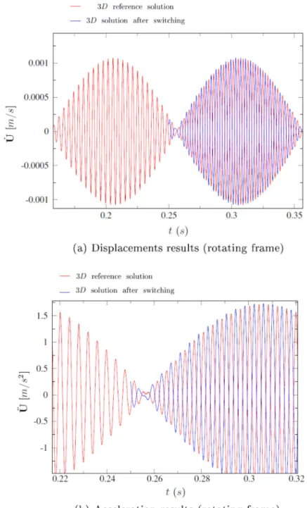
Velocities and accelerations are presented in Fig. 16.
A simple comparison between Figs. 7 and 15 shows that the response of the rotor has the same modulations frequency as the preceding example. However, it is obvious, especially on Figs. 7b and 15b, that the amplitudes of those modulations are increased due to the increased rotating velocity (from 300 rpm to 1500 rpm). The loading time law is not the only factor that can increase the amplitude of the response. The rotation velocity is a key factor.
Fig. 16. Velocities and accelerations results (rotating frame).
Analyzing the energy curves illustrates the robustness of the switch on higher rotational velocity cases. For a better clarity, the kinetic energy is presented in the time interval t ∈ [0.2 s, 0.3 s] in Fig. 17. It is obvious that the kinetic energy of the 3D switch solution is closer to that of the beam model than to that of the 3D reference solution. Differences exist between the beam and the 3D reference solutions, for the reasons previously discussed.
At the switch instant, the 3D switch solution clings on the beam one. This explains why the kinetic energy of the 3D switch solution (for both the components: the component resulting from the overall rotation and the one due the vibration of the rotor around its stable equilibrium position) is closer to that of the beam one than to that to the 3D reference solution kinetic energy.
This can be less visible on the strain energy (see Fig. 18). The strain energy of the 3D switch solution is very close to that of the 3D reference solution. The total energy is constant and do not present any perturbation. The 3D reference solution and the 3D switch solution have practically the same total energy as illustrated by Fig. 19.
The increase in the rotational velocity leads to more intensified vibrations of the rotor. However, the switch method preserve its accuracy and robustness.
Fig. 18. Strain energy for ω = 1500 rpm.
We thereafter, present a third and last application example for which the rotation velocity is ω = 300 rpm, but the loading is imposed progressively on a 0.1 s time interval (see Fig. 6). The following results are obtained on point PN in the rotating frame.
Fig. 20 shows the displacements results on point PN, while Fig. 21 shows the velocities and acceleration
results of point PN around the switch instant in the rotating frame.
Fig. 20. Displacements results for the second loading law (rotating frame).
In the following a comparison of this study case with the first one, i.e., with an imbalance established on 0.01 s and a 300 rpm rotational velocity is performed. By comparing the displacements of the first study case (Fig. 20) and those of this study case (Fig. 7b), one can conclude that imposing the imbalance progressively reduces the amplitudes of the modulations. However, the modulations retain the same natural frequency in both the study cases.
This fact is also highlighted by comparing the velocities and accelerations of the two study cases, i.e., by comparing Figs. 9a and 21a.
In this study case, due to a smoother application of the imbalance, the rotor vibrates less violently around its stable equilibrium position. The kinetic and strain energies (Fig. 23) show small oscillations. The switch does not perturb the energetic stability of the system (no parasite energy is inserted nor removed, no oscillations are found on the energy curves, etc.). Moreover, a closer look to the kinetic energy curve Fig. 22 shows that in spite of the weakness of the kinetic energy component that counts for the vibration of the rotor around its stable equilibrium position Wcd, with respect to the component that count for the overall
rotation Wcr, i.e., Wcd≪ Wcr, the switch does not introduce parasite energy in any of the components.
Fig. 21. Velocities and accelerations results for the second loading law (rotating frame).
Fig. 23. Strain energy for the second loading law.
Fig. 24. Total energy for the second loading law.
5. Limits of the strategy
The presented strategy is simple, efficient and easy to implement for the different applications considered previously. However, one may demand if for some application cases, the switch method will not work or lead to unreliable results. This section presents an insight into the theoretical conditions that, if accomplished, make the switch efficient for any type of application, even for complex geometries, loads, boundary conditions, etc. These conditions, as explained later, can be resumed by the necessity of having the orthogonality of vectors and . Moreover, understanding the strategy’s limits begins by examining the causes that make it difficult to strictly satisfy this condition.
5.1. Optimal strategy if the orthogonality of vectors and is satisfied
Switching from the beam to the 3D model, according to the first switching strategy, leads to a transient stage depicted by high frequency oscillations that can be attenuated by numerical damping.
This is why strategy two was proposed. The latter, thanks to velocities and accelerations corrections make it possible to switch correctly without passing through a transient stage. Let us first discuss the main causes that are behind the transient stage that appear after switching when the first strategy is used and then discuss why strategy two is better and finish by understanding what are the possible limits of strategy two.
The basics of the switch is that results from a beam computation that is based on a rigid body assumption, and is a 3D correction that accounts for a rigid-body cross-section deformation. Therefore, the two vectors should be orthogonal. In other words, since is a pure 3D solution, then its construction should not depend on , since the latter is generated from a beam solution. It also means that counts only for the cross-section deformation and is not related to the beam deflection, since the later is taken into account in .
The fundamental equation of motion of a 3D model at t = ts is described by:
(15)
From we obtain:
(16)
It can be demonstrated that if we have a coincidence between the beam and the 3D models shape functions, in addition to very fine meshes and a non-lumped 3D mass matrix, then we can write:
(17)
as well as .
Taking into account that is the beam solution which fulfills , then Eq.
(16) leads to:
(18)
Since we have the assumption and (see Eq. (8)), we obtain the following orthogonality condition:
(19)
As explained earlier, the computation of PT turns to be cumbersome, so that the orthogonality condition will be written as follows:
∀ , (20)
Having the orthogonality of vectors and satisfied implies that the construction of vector does not depend on the beam solution. In other words, is a vector that counts for the cross-section deformation but is not related to the beam deflection since that latter is taken into account in the beam solution.
Satisfying the orthogonality condition implies practically that the 3D solution at the switch instant has exactly the same deflection as the beam solution. is a correction vector that brings the required complementary information for the construction of the 3D solution, i.e., the cross-section deformation.
However, Eq. (17) are practically never satisfied. The main difficulty is not having non lumped mass matrices (it is possible in most finite element software), but in the compatibility of the beam and 3D shape functions. However, a sufficient fine 3D mesh contributes to a better approximation of Eq. (17).
The orthogonality condition can also be seen from a different point of view, that of the contribution of each solution component ( and ), in the deformation energy of the 3D solution at the switch instant.
A closer look into the strain energy of the beam and the 3D models will give a better significance of the orthogonality condition, and of the meanings of it to be verified or not.
The strain energy of the beam model is:
(21)
The deformation energy of the 3D model taking into account the symmetry of the stiffness matrix is:
(22)
from the orthogonality condition and Eq. (17) one has:
(23)
thus the strain energy of the 3D model is equal to the strain energy corresponding to the cross-section deformation and the strain energy of the beam. Therefore, when switching no parasite energy should appear.
5.2. Non verifying the orthogonality condition consequences
The orthogonality condition cannot be respected unless Eq. (17) are true. However, due to the difference in the shape functions used for a beam model and those used for a 3D one (the space discretization is not hierarchically nested), it is not possible to satisfy the orthogonality condition of and exactly. Thus, and that implies that, when the first switching strategy is considered, a parasite energy is created when switching and is depicted by high frequency oscillations that appear immediately after switching and are attenuated by numerical damping. Not verifying the orthogonality condition also means that the beam deflection and the 3D reference model deflection at the switch instant are not equal. This fact can be seen in all the illustrative applications of this article (see for example Figs. 10 and 11) and is schematized in Fig. 25. It is due to the fact that the natural frequencies of the two models are very close but not equal.
The switch leads to a 3D solution that is equivalent but not equal to the reference one. When the triple static switch is considered, the difference between the 3D reference solution and the beam solution leads no more to a transient stage since the difference is compensated by velocities (and subsequently accelerations) corrections. Thus, no numerical damping is needed.
5.3. Limits of the strategy: discussion and examples
When the difference between the beam and the 3D solution is very important, the switch has no meaning and that is the main limit of the strategy.
In the following, the previous rotor with same loading and boundary conditions is considered. It is set to rotate at ω = 15 000 rpm (equivalent to 250 Hz). This velocity is very close to a natural frequency of the rotor. In fact, the beam rotor has a natural frequency of 253.76 Hz while its equivalent for the 3D one is 255.59 Hz. Even though the difference is small and is due to normal modeling differences (see Section 5.2), this will lead to non-negligible behavior differences as shown in Fig. 26. In such a case, the switch should not be performed. Note, however, that this difference does not lead the switch to diverge, but rather to a solution that is different from both. However, switching is useful when the beam and the 3D models give similar results which here means at a rotation speed sufficiently far from natural frequencies.
Fig. 26. Different behavior of a beam and a 3D model simulating the same physical problem and loading.
When the triple static switch is performed, no parasite energy is introduced in the system. The efficiency of the switch is not reduced, if lot of physical high frequencies are excited. It is only the difference between the beam and the 3D solution that may limit the switch. It can be reduced when the rotor is sufficiently slender, the 3D mesh is fine, etc.
The main advantage of the switch is its ease of implementation and none intrusive aspect. However, an intrusive switch in which the orthogonality of and is overcome is to be proposed in a future publication.
6. Conclusions
This article proposes a strategy that enables one to reduce the computational cost for the simulation of the accidental slowing down of turbines. This strategy is simple, efficient, robust and preserve the accuracy when a 3D description is required only on a small part time domains.
Despite an inevitable phase shift between the 3D reference solution and the beam solution, the switch enables to produce a 3D solution that represents a good approximation of the 3D reference solution. This 3D switch solution is initialized from the beam solution and has the same natural frequencies of the 3D reference solution. The proposed approach is also energetically sound and enables a significant computational cost saving.
Although this article illustrated the switch from a beam model to a full 3D model, limiting the size of the 3D zone to the area where non-linear phenomena is to take place can be achieved by performing a switch from a beam model to a hybrid beam-3D model. A hybrid beam-3D model can be obtained as done in Tannous et al [36].
This switch method can be applied to more diverse applications, such as local plasticity or thermo-plasticity, cracking, and several other kinds of local linear or non-linear effects as long as the switch is performed in the linear stage preceding any non-linearity.
The switch is a non-intrusive approach that was developed on Code_Aster, and can be easily implemented on a commercial finite element software.
Acknowledgments
The authors thank the French National Research Agency (ANR) in the frame of its Technological Research COSINUS Program. (IRINA, Project ANR 09 COSI 008 01 IRINA).
Appendix A. Generating
is obtained through a projector matrix P which transforms the beam displacement vector into a 3D rigid body displacement per beam section. It is noteworthy to say that the 3D mesh and the beam mesh cannot be totally disconnected in order for the switch to be done. To be able to construct the displacement of a node on the 3D mesh, we should have the displacements and rotations of the beam node that has the same position along the beam. In other words, the beam model should be a projection of the 3D mesh on its neutral axis. However, it is not easy to build P because it depends on the relationship between the beam mesh and the 3D mesh, which may change from one cross-section to another. Instead, we will generate
as a whole.
Let n the number of cross-sections. Gi, with i = 1…n, is a point belonging to the neutral axis of the
cross-section i. Each cross-cross-section of the 3D beam model is constituted of mi 3D nodes. Note that the number of
nodes may differ from one cross-section to another. Nij, with j = 1…mi is a node that belongs to the ith
cross-section of the 3D model.
is the displacement of Nij computed for a cross-section rigid body displacement. The cross-section
to which belongs Nij has Gi on its neutral axis. The ith beam node, which has the same coordinates as Gi, has
a displacement and a rotational displacement . With the finite element software used, such as
Code_Aster or Abaqus, we write a python loop that manages to compute , , for each node Nij as follows:
where is a vector oriented from Nij to Gi. Point Nij has , , for coordinates. Suppose
0, therefore Eq. (A.1) reads:
−
(A.2)
−
References
[1] Narasimhan N, Lovell M. Predicting springback in sheet metal forming: an explicit to implicit sequential procedure. Finite Elem Anal Des 1999;33:29–42.
[2] Jung D, Yang D. Step-wise combined implicit–explicit finite element simulation of autobody stamping processes. J Mater Process Technol 1998;83:245–60.
[3] Lo C, Hinnerichs T, Hales J. Assessment of efficiency for a hybrid explicit/ implicit code simulation of a multiple impact crash scenario. In: Proceedings of 2005 ASME international mechanical
engineering congress and exposition; 2005, p. 381–6.
[4] Noels L, Stainier L, Ponthot J-P, Boinini J. Combined implicit–explicit algorithms for non-linear structural dynamics. Rev Euro Élém Finis 2002;11:565–91.
[5] Noels L, Stainier L, Ponthot J-P, Bonini J. Automatic time stepping algorithms for implicit numerical simulations of non-linear dynamics. Adv Eng Softw 2002;33:589–603.
[6] Noels L, Stainier L, Ponthot J-P. Combined implicit/explicit algorithms for crashworthiness analysis.
Int J Impact Eng 2004;30:1161–77.
[7] Noels L, Stainier L, Ponthot J-P. Combined implicit/explicit time-integration algorithms for the numerical simulation of sheet metal forming. J Comput Appl Math 2004;168:331–9.
[8] Noels L, Stainier L, Ponthot J-P, Bonini J. Automatic time stepping algorithms for implicit numerical simulations of blade/casing interactions. Int J Crashworthiness 2001;6:351–62.
[9] Mahjoubi N, Gravouil A, Combescure A. Coupling subdomains with heterogeneous and incompatible time steps. Comput Mech 2009;44:825–43.
[10] Hirai I. An exact zooming method for finite element analyses. In: NASA conference publication, vol. 2245, 1982.
[11] Hirai I, Uchiyama Y, Mizuta Y, Pilkey W. An exact zooming method. Finite Elem Anal Des 1985;1:61–9.
[12] Plaza A, Padron MA, Carey GF. A 3D refinement/derefinement algorithm for solving evolution problems. Appl Numer Math 2000;32:401–18.
[13] Ben Dhia H. Multiscale mechanical problems: the Arlequin method. Mech Solids Struct 1998;326:899–904.
[14] Ben Dhia H, Rateau G. The Arlequin method as a flexible engineering design tool. Int J Numer
Methods Eng 2005;62:1442–62.
[15] Cottereau R, Clouteau D, Dhia HB, Zaccardi C. A stochastic–deterministic coupling method for continuum mechanics. Comput Methods Appl Mech Eng 2011;200:3280–8.
[16] Ghanem A, Mahjoubi MTN, Baranger T, Combescure A. Arlequin framework for model, multi-time scale and heterogeneous multi-time integrators for structural transient dynamics. Comput Methods
Appl Mech Eng 2013;254:292–308.
[17] Kettil P, Wiberg N-E. Application of 3D solid modeling and simulation programs to a bridge structure. Eng Comput 2002;18:160–9.
[18] Lions J-L, Pironneau O. Domain decomposition methods for CAD. CR Acad Sci Paris Sér I – Math 1999;328:73–80.
[19] Glowinski R, He J, Lozinski A, Rappaz J, Wagner J. Finite element approximation of multi-scale elliptic problems using patches of elements. J Numer Math 2005;101:663–87.
[20] He J, Lozinski A, Rappaz J. Accelerating the method of finite element patches using approximately harmonic functions. CR Math Acad Sci Paris 2007;345:107–12.
[21] Mandel J. Balancing domain decomposition. Commun Numer Methods Eng 1993;9:233–41.
[22] Farhat C, Roux FX. A method of finite element tearing and interconnecting and its parallel solution algorithm. Int J Numer Methods Eng 1991;32:1205–27.
[23] Farhat C, Lesoinne M, Le Tallec P, Pierson K, Rixen D. FETI-DP: a dual-primal unified FETI method – Part I: A faster alternative to the two-level FETI method. Int J Numer Methods Eng 2001;50(7):1523–44.
[24] Mobasher Amini A, Dureisseix D, Cartraud P, Buannic N. A micro–macro strategy for ship structural analysis with FETI-DP method. In: 3rd European conference on computational mechanics: solids,
structures and coupled problems in engineering, Lisbon, Portugal, 2006, p. 233–40.
[25] Mobasher Amini A, Dureisseix D, Cartraud P. Multi-scale domain decomposition method for large-scale structural analysis with a zooming technique: application to plate assembly. Int J Numer
Methods Eng 2009;79:417–33.
[26] Ladevèze P, Loiseau O, Dureisseix D. A micro–macro and parallel computational strategy for highly heterogeneous structures. Int J Numer Methods Eng 2001;52:121–38.
[27] Farhat C, Pierson K, Lesoinne M. The second generation FETI methods and their application to the parallel solution of large-scale linear and geometrically non-linear structural analysis problems.
Comput Methods Appl Mech Eng 2000;184:333–74.
[28] Avery P, Rebel G, Lesoinne M, Farhat C. A numerically scalable dual–primal substructuring method for the solution of contact problems Part I: The frictionless case. Comput Methods Appl Mech Eng 2004;193:2403–26.
[29] Avery P, Farhat C. The FETI family of domain decomposition methods for inequality-constrained quadratic programming: application to contact problems with conforming and nonconforming interfaces. Comput Methods Appl Mech Eng 2009;198:1673–83.
[30] Dureisseix D, Farhat C. A numerically scalable domain decomposition method for the solution of frictionless contact problems. Int J Numer Methods Eng 2001;50:2643–66.
[31] Alart P, Barboteu M, Le Tallec P, Vidrascu M. Additive Schwarz method for nonsymmetric problems: application to frictional multicontact problems. Domain Decompos Methods Sci Eng 2002:3–13.
[32] Gendre L, Allix O, Gosselet P, Compte F. Non-intrusive and exact global/local techniques for structural problems with local plasticity. Comput Mech 2009;44:233–45.
[33] Gendre L, Allix O, Gosselet P. A two-scale approximation of the Schur complement and its use for non-intrusive coupling. Int J Numer Methods Eng 2011;87:889–905.
[34] Andrieux S, Varé C. A 3D cracked beam model with unilateral contact. Application to rotors. Eur J
Mech A/Solids 2002;21:793–810.
[35] Roques S, Legrand M, Cartraud P, Stoisser C, Pierre C. Modeling of a rotor speed transient response with a radial rubbing. J Sound Vib 2009;329: 527–46.
[36] Tannous M, Cartraud P, Dureisseix D, Torkhani M. A beam to 3D model switch for transient dynamic analysis. Finite Elem Anal Des 2014;91: 95–107.
[37] Tannous M, Cartraud P, Dureisseix D, Torkhani M. A beam to 3D model switch for transient dynamic analysis. In: Proceedings of the 6th European congress on computational methods in applied
[38] Tannous M. Développement et évaluation d’approches de modélisation numérique couplées 1D et 3D du contact rotor–stator. Ph.D. thesis, Ecole Centrale de Nantes; 2013.
[39] EDF R&D: Code_Aster: a general code for structural dynamics simulation under GNU GPL licence; 2001. <http://www.code-aster.org>.
[40] Ghanem A. Contributions à la modélisation avancée des machines tournantes en dynamique transitoire dans le cadre Arlequin. Ph.D. thesis, l’Institut National des Sciences Appliquées de Lyon; 2013.
[41] Lalanne M, Ferraris G. Dynamique des Rotors en Flexion, Ed. Techniques Ingénieur; 1996.
[42] Hilber H, Hughes T, Taylor R. Improved numerical dissipation for time integration algorithms in structural dynamics. Earthq Eng Struct Dyn 1977;5:283–92.
[43] Géradin M, Rixen D. Mechanical vibrations: theory and application to structural dynamics. John Wiley and Sons; 1994.