A new formulation of equivalent effective stratospheric chlorine (EESC)

(1)

HAL Id: hal-00302668

https://hal.archives-ouvertes.fr/hal-00302668

Submitted on 22 Mar 2007

HAL is a multi-disciplinary open access

archive for the deposit and dissemination of sci-entific research documents, whether they are pub-lished or not. The documents may come from teaching and research institutions in France or abroad, or from public or private research centers.

L’archive ouverte pluridisciplinaire HAL, est destinée au dépôt et à la diffusion de documents scientifiques de niveau recherche, publiés ou non, émanant des établissements d’enseignement et de recherche français ou étrangers, des laboratoires publics ou privés.

A new formulation of equivalent effective stratospheric

chlorine (EESC)

P. A. Newman, J. S. Daniel, D. W. Waugh, E. R. Nash

To cite this version:

P. A. Newman, J. S. Daniel, D. W. Waugh, E. R. Nash. A new formulation of equivalent effec-tive stratospheric chlorine (EESC). Atmospheric Chemistry and Physics Discussions, European Geo-sciences Union, 2007, 7 (2), pp.3963-4000. �hal-00302668�

(2)

ACPD

7, 3963–4000, 2007 New formulation of EESC Newman et al. Title Page Abstract Introduction Conclusions References Tables Figures ◭ ◮ ◭ ◮ Back Close

Full Screen / Esc

Printer-friendly Version

Interactive Discussion

EGU Atmos. Chem. Phys. Discuss., 7, 3963–4000, 2007

www.atmos-chem-phys-discuss.net/7/3963/2007/ © Author(s) 2007. This work is licensed

under a Creative Commons License.

Atmospheric Chemistry and Physics Discussions

A new formulation of equivalent effective

stratospheric chlorine (EESC)

P. A. Newman1, J. S. Daniel2, D. W. Waugh3, and E. R. Nash4 1

Atmospheric Chemistry and Dynamics Branch, NASA Goddard Space Flight Center, Greenbelt, Maryland, USA

2

NOAA Earth System Research Laboratory/Chemical Sciences Division, Boulder, Colorado, USA

3

Johns Hopkins University, Baltimore, Maryland, USA 4

Science Systems and Applications, Inc., Lanham, Maryland, USA

Received: 27 February 2007 – Accepted: 19 March 2007 – Published: 22 March 2007 Correspondence to: P. A. Newman (paul.a.newman@nasa.gov)

(3)

ACPD

Full Screen / Esc

EGU

Abstract

Equivalent effective stratospheric chlorine (EESC) is a convenient parameter to quan-tify the effects of halogens (chlorine and bromine) on ozone depletion in the strato-sphere. We show and discuss a new formulation of EESC that now includes the effects of age-of-air dependent fractional release values and an age-of-air spectrum. This new

5

formulation provides quantitative estimates of EESC that can be directly related to inor-ganic chlorine and bromine throughout the stratosphere. Using this EESC formulation, we estimate that human-produced ozone depleting substances will recover to 1980 levels in 2041 in the midlatitudes, and 2067 over Antarctica. These recovery dates are based upon the assumption that the international agreements for regulating

ozone-10

depleting substances are adhered to. In addition to recovery dates, we also estimate the uncertainties in the estimated time of recovery. The midlatitude recovery of 2041 has a 95% confidence uncertainty from 2028 to 2049, while the 2067 Antarctic recov-ery has a 95% confidence uncertainty from 2056 to 2078. The principal uncertainties are from the estimated mean age-of-air, and the assumption that the mean age-of-air

15

and fractional release values are time independent. Using other model estimates of age decrease due to climate change, we estimate that midlatitude recovery may be accelerated from 2041 to 2031.

1 Introduction

Ozone-depleting substances (ODSs) are primarily comprised of chlorine- and

bromine-20

containing chemicals that have very long lifetimes in the atmosphere. These human produced ODSs have now been regulated under the landmark 1987 Montreal Pro-tocol agreement and the amendments and adjustment to the ProPro-tocol (Sarma and Bankobeza, 2000). Based upon ground measurements and emission estimates, the future ground levels of ODSs has been developed as scenario A1 in WMO (2007).

25

(4)

ACPD

Full Screen / Esc

EGU a steady decline of most ODSs over the coming decades.

Due to the established relationship between stratospheric ozone depletion and in-organic chlorine and bromine abundances, the temporal evolution of chlorine- and bromine-containing halogenated species is an important indicator of the potential dam-age of anthropogenic activity on the health of stratospheric ozone. Equivalent effective

5

stratospheric chlorine (EESC) was developed to relate this halogen evolution to tro-pospheric source gases in a simple manner (Daniel et al.,1995). This quantity sums ODSs, accounting for a transit time to the stratosphere, for the greater potency of stratospheric bromine (Br) compared to chlorine (Cl) in its ozone destructiveness with a constant factor (α), and also includes the varying rates with which Cl and Br will be 10

released in the stratosphere from different source gases (i.e., fractional release, f ). The fractional release accounts for ODS disassociation in the stratosphere relative to the amount that entered at the tropopause. EESC has been used to relate predictions of human-produced ODS abundances to future ozone depletion (WMO,1995,1999, 2003,2007).

15

In the past, EESC estimates have been used to evaluate various ODS emission sce-narios primarily using two metrics. These include 1) a comparison of the times when EESC returns to 1980 levels and 2) the relative integrated changes in EESC between 1980 or some other time and when EESC returns to 1980 levels. These comparison metrics did not require that EESC quantitatively describe stratospheric chlorine and

20

bromine levels, but only that it be proportional to these levels. Furthermore, these EESC calculations had not included a distribution of transport times from the tropo-sphere into the stratotropo-sphere (the so called age-of-air spectrum) or any dependence of the fractional chlorine release values on the age-of-air. As air moves into the strato-sphere at the tropical tropopause ODSs have not been disassociated, and have

frac-25

tional release values near zero. In contrast, after transiting through the upper strato-sphere, the ODSs in an air parcel are nearly fully disassociated and have fractional release values close to 1.0. Recently, Newman et al. (2006) reformulated EESC to account for both an age-of-air spectrum and age dependent fractional release values.

(5)

ACPD

Full Screen / Esc

EGU This new formulation provides quantitative estimates of inorganic chlorine, bromine,

fluorine, and EESC, for different regions of the stratosphere. The purpose of this paper is to further articulate this new formulation and to expose some of the uncertainties in the calculation of EESC. These uncertainties can have considerable impact on ODS recovery dates.

5

In addition to recovery estimates, EESC has been used as a proxy for halogen levels in ozone trend analysis studies (Yang et al.,2005;Dhomse et al.,2006;Guillas et al., 2006;Newman et al.,2006;Stolarski et al.,2006b). Past trend analysis studies used a linear trend to represent the effects of ODS changes, however with the regulation of ODSs, a linear trend is no longer appropriate. Most trend studies now use EESC

10

as an ODS proxy because stratospheric ozone depletion trends are changing, and these changes most probably began when halogen levels stopped increasing in the late 1990s (Montzka et al.,1996). A few of these studies have suggested that ozone recovery has now passed its first stage: i.e., the linear decrease has stopped and ozone levels are no longer dropping (e.g.,Newchurch et al.,2003;WMO,2007). It is

15

critical that assumptions that are hidden, but implicit in EESC estimates, be understood in order to properly apply EESC in an ozone trend analysis and to ascribe ozone trend changes to the regulation of ODSs.

This paper is divided into six sections. Section2provides the theoretical description of EESC in both its new formulation and in the formulation used in past assessments.

20

In the remainder of this paper, we will separately refer to the “classic EESC” used in the WMO assessments and to the reformulated EESC used byNewman et al.(2006). Section3shows a step-by-step construction of reformulated EESC, and Sect.4 com-pares this reformulation to the classic EESC. Section 5 has detailed descriptions of reformulated EESC uncertainties. The final section summarizes and discusses the

25

(6)

ACPD

Full Screen / Esc

EGU

2 Equivalent effective stratospheric chlorine (EESC)

EESC, as a function of timet, is defined as

EESC(t) = a X Cl n_if_iρ_i + αX Br n_if_iρ_i ! , (1)

wheren is the number of chlorine or bromine atoms of a particular source gas i, f

represents the efficiency of stratospheric halogen release of the source gas relative to

5

that of chloroflurocarbon-11 (CFC-11), andρ is the source gas mixing ratio when the

gas entered the stratosphere (Daniel et al.,1995). Summations are over the Cl- and Br-containing halocarbons. The leading factor,a, can be an arbitrary value as indicated

byWMO(1995,1999,2003,2007) or it can be the fractional release value of CFC-11 so that the EESC quantity accurately represents the amount of inorganic chlorine (Cly)

10

and bromine (Br_y) in some region of the stratosphere. In the rest of this manuscript, we fold thea factor directly into the f values. Equivalent effective chlorine (ECl) (Montzka et al., 1996) represents the same quantity but with no consideration of the transport time to the stratosphere and all fractional releases set to a value of 1.0.

In the classic EESC,ρ_i is calculated assuming a simple time lag, Γ, from the surface

15

observations

ρ_i = ρi ,entry(t − Γ) , (2)

whereρ_{i ,entry}(t) is the surface observation at time t. WMO(1995,1999,2003,2007) estimated this classic EESC assuming Γ = 3 y to obtain a value appropriate for relating to globally averaged ozone loss.

20

The relative effectiveness of bromine compared to chlorine for ozone depletion (α in Eq. 1), arises from the residence of inorganic bromine in more active compounds for ozone destruction. This relative effectiveness is usually presented for global ozone depletion although it is a function of altitude, latitude, and background chlorine and bromine amount. We adopt a value of 60 for α in both EESC formulations following 25

(7)

ACPD

Full Screen / Esc

EGU WMO (2007) and refer to the detailed discussion in that assessment regarding the

update of this value from the value of 45 assumed byWMO(2003).

EESC estimates were reformulated by Newman et al. (2006). They revised the method of calculating EESC to account for the fact that 1) different stratospheric lo-cations are characterized by different mean transit times, 2) each location is composed

5

of air characterized by not a single transit time, but a range, and 3) the fractional re-lease values depend on the mean age of air. In theNewman et al.(2006) calculations

ρi is calculated using age-of-air spectra weighted mixing ratios as

ρ_i(t) =

Zt −∞

ρ_i,entry(t′₎_{G(t − t}′₎_{d t}′_, ₍₃₎ whereG(t) is the age-spectrum, and the fractional releases are age-of-air dependent, 10

fi = fi(Γ). This reformulation reduces to the classic EESC calculation if G(t) = δ(t − Γ),

a delta function, and Γ = 3 y. This just represents a forward shift of the entire time series ofρ_i,entry(t) by 3 years.

Estimates of total inorganic and organic chlorine and bromine can be provided from Eq. (1). The first term in Eq. (1) provides an estimate of Cly, while the second term

15

(withoutα) is an estimate of Bry. In addition, the reformulated equation can be used to estimate total inorganic fluorine by using the number of fluorine atoms in each species, and the same tropospheric mixing ratios and fractional release values.

In Eq. (1),f represents the fraction of the species that has been disassociated during

its movement through the stratosphere. Fractional release was originally defined by

20

Solomon and Albritton(1992) as:

fi =

ρi ,entry− ρi,φ,θ

ρ_{i ,entry} , (4)

where φ is latitude and θ represents altitude (or potential temperature). In Eq. (1), it is assumed that f is mainly dependent on mean age-of-air and is independent of

(8)

ACPD

Full Screen / Esc

EGU mean age-of-air from lower stratospheric aircraft observations. Observational based

fractional release values for other species in the lower stratosphere were derived by Newman et al.(2006).

To apply Eq. (1) to Eq. (3) it is necessary to know the mean age-of-air and, in the case of Eq. (3), the age spectrum. Calculations of mean ages from observations of carbon

5

dioxide (CO2) or sulfur hexafluoride (SF6) indicate that in the lower stratosphere the mean age is around 3 years in midlatitudes and around 5.5 years in polar regions (e.g., Waugh and Hall,2002;Newman et al.,2006, and references therein), and we use these values in our standard calculations. There is some uncertainty in the characteristics of the full age spectrum, although analysis of multiple tracers indicates that the spectra

10

are broad (e.g.,Andrews et al.,2001;Schoeberl et al.,2005). In our calculations we assume that the age spectrum is an inverse Gaussian function with mean, Γ, and width, ∆ (see Eq. (9) ofWaugh and Hall,2002), related by ∆ = Γ/2. The sensitivity to this value of ∆/Γ is examined below.

3 Estimating EESC

15

In this section, we will show the details of estimating the reformulated EESC. We start with a time history of CFC-11 mixing ratio measurements and expected future concen-trations. Figure1 displays this CFC-11 time history of chlorine using scenario A1 of WMO(2007). The surface observations (black) of the chlorine contained in CFC-11 are multiplied by 3 to account for the three chlorine atoms (niρi in Eq.1). The peak CFC-11

20

surface value of 809.1 ppt of chlorine occurs in 1994 shortly after the 1992 production phaseout during the 1993–1994 period (WMO,2007). The figure also shows the chlo-rine from CFC-11 after the application of a 3-year age spectrum (Γ = 3 y, ∆ = 1.5 y, red dashed) and a 5.5-year age spectrum (Γ = 5.5 y, ∆ = 2.75 y, blue dashed) to the surface time series using Eq. (3). The age spectrum shifts the time series to later times

25

as would be expected. While the surface CFC-11 peaked in 1994, the CFC-11 in the stratosphere for 3-year old air peaked in 1998. For 5.5-year old air, the peak is shifted

(9)

ACPD

Full Screen / Esc

EGU to 2001 and the maximum is reduced to about 788 ppt. This shift is slightly later than

that obtained from a simple 5.5-year shift and the peak is smaller than the surface peak because of the consideration of the age spectrum. The peak value in 2001 results from the 5.5-year age spectrum weighted average of surface values prior to 2001. Since, most of those surface values are considerably less than the 809.1 ppt peak, the peak

5

in 2001 must be smaller than the size of the surface peak.

The fractional release, f , provides the fractional amount of CFC-11 that has been

dissociated in the stratosphere relative to the amount that entered at the tropopause. Schauffler et al.(2003) used ER-2 observations to calculate the fractional release of CFC-11 as a function of mean age-of-air. The release of chlorine via the degradation

10

of CFC-11 in the stratosphere occurs by solar photolysis at wavelengths less than approximately 240 nm. At the tropical tropopause (air that has recently entered the stratosphere), virtually none of the CFC-11 has been degraded. Hence, its fractional release is zero. For a 3-year mean age of air, approximately 47% of the CFC-11 has been converted into inorganic chlorine, with 53% remaining as CFC-11. For a 5.5-year

15

mean age-of-air, essentially all of the CFC-11 has been converted. The solid red curve of Fig.1displays the Cl_ycontribution from CFC-11 (nifiρi in Eq.1).

Table 1 lists 16 different species used to estimate EESC in this study along with their chemical formulas, year 2000 surface mixing ratios fromWMO (2007) scenario A1, estimated lifetimes, and observationally derived fractional release values for 3- and

20

5.5-year mean ages (valid in the lower stratosphere).

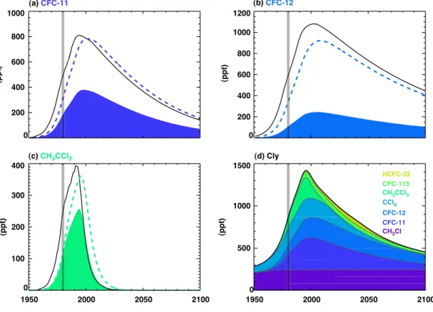
Cly is estimated by summing the contributions of all the long-lived chlorine species. Short-lived chlorine containing gases may contribute approximately 100 ppt to Cl_y (WMO,2007), but their contribution is not included herein. Figure 2displays the con-tributions from CFC-11, CFC-12, and methyl chloroform to total chlorine. Figure 2a

25

is identical to Fig. 1, shown again for ease of comparison with CFC-12 and methyl chloroform. Figures2a–c, show surface concentrations (black), the inorganic contri-bution to Cly for a 3-year mean age-of-air (filled), and the inorganic contribution to Cly for a 5.5-year mean age-of-air (dashed). The fractional release values are qualitatively

(10)

ACPD

Full Screen / Esc

EGU related to the inverse of stratospheric lifetimes of the species. Stratospheric lifetimes

for CFC-11, CFC-12, and methyl chloroform are 45 y, 100 y, and 49 y, respectively. For a 3-year mean age, the associated fractional releases are 0.47, 0.23, and 0.67, respectively (Table1). The cumulative sum is shown in Fig. 2d. On a time average, the species that contribute the majority of the chlorine to the stratospheric inorganic

5

burden are: methyl chloride, CFC-11, CFC-12, carbon tetrachloride, methyl chloro-form, CFC-113, and HCFC-22. Methyl chloride is the dominant natural species that contributes to stratospheric chlorine. An additional five Cl-containing species are in-cluded in Fig.2d, but their contributions are too small to be clearly displayed. For air in the stratosphere with a 3-year mean age-of-air, Cl_yhad a peak value in mid-1995 at

10

approximately 1420 ppt.

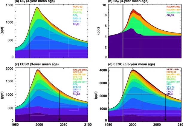
As indicated in Eq. (1), EESC is estimated by combining the inorganic chlorine with inorganic bromine. Bromine is a more efficient depleter of ozone, and is scaled by

α=60. Figure3 displays Cl_y, Br_y, and EESC. Figure 3a is the same as Fig.2d (with color rearrangement) for a 3-year mean age-of-air. Bry peaks in 2001, about six years

15

later than Cly, with a maximum value of 9.1 ppt. The reformulated EESC in Fig.3c is combined from Fig.3a and Fig.3b. Figure3d is similar to Fig.3c, but is calculated for a 5.5 year mean age-of-air.

The EESC is characterized by both a strong variation of magnitude and peak year between the 3-year curve (Fig. 3c) and the 5.5-year curve (Fig. 3d). The reference

20

year of 1980 is often chosen as a metric for substantial recovery (gray vertical line). The year of recovery (black vertical line) of EESC is then considered to be when the EESC value drops to the same as in the reference year (black horizontal line). This recovery of EESC would occur in 2041.3 for a 3-year (Fig.3c) and in 2067.2 for a 5.5-year (Fig. 3d) mean age-of-air. The peak values of EESC are substantially different

25

between a 3- and a 5.5-year mean age. The 3-year mean age EESC value peaks at 1931 ppt in mid-1996, while the 5.5-year mean age EESC peaks at a value of 4045 ppt in early 2001.

(11)

ACPD

Full Screen / Esc

EGU

4 Comparison with classic EESC

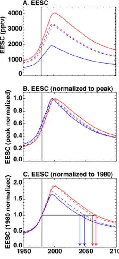
The classic EESC used byWMO(1995,1999,2003,2007) is formulated as shown in Eq. (1), but it uses the simple time series shift noted above and uses different values for the fractional release values than are used bySchauffler et al.(2003) andNewman et al. (2006). Figure4displays the EESC estimated in the reformulation (solid) and the

5

classic technique (dashed) using Γ=3 y (blue) and Γ = 5.5 y (red). Figure4a shows the actual values of EESC as calculated by the two techniques, where the reformulated EESC curves yield a quantitative estimate (i.e., Cly and Bry) while the classic EESC does not.

Figure 4b shows the EESC curves normalized to the respective peak values. For

10

Γ = 3 y, the classic EESC behavior is similar to the reformulated EESC. However, for Γ=5.5 y, there is a significant difference between reformulated and classic EESC in the period after approximately 2001. This difference results from the higher “relative to 1980” peak value of the classic EESC in 2000 that can be seen in Fig.4c.

As noted in Table1, differing fractional release values will impact the estimated

re-15

covery date. Because of these release differences, recovery estimates here are dif-ferent from those reported byWMO (2007). For a 3-year shift in the classic EESC, WMO (2007) estimated a 2048.8 recovery in comparison to our reformulated EESC estimate of 2041.3 (a difference of 7.5 y). Only a small part of this difference is due the application of an age spectrum: if we use the simple 3-year shift, rather than an

20

age spectrum, with our age dependent release rates the difference fromWMO(2007) is 7.0 y. For a 6-year shift,WMO(2007) calculated a 2064.7 recovery. If we use their 6-year mean age with our reformulated EESC, we estimate recovery in 2073.3. Hence, recovery differences between our estimates andWMO(2007) are primarily related to fractional release value differences.

25

The reasons for the differences between our reformulated EESC fractional release values (Schauffler et al.,2003;Newman et al.,2006) and theWMO(2003,2007) re-lease values are currently uncertain. There are particularly striking differences in the

(12)

ACPD

Full Screen / Esc

EGU values for HCFC-141b and HCFC-142b. The derivation of these values from data

(Schauffler et al.,2003) is quite sensitive to an accurate assessment of the age-of-air for gases such as these with a large trend. However, the uncertainty in the age inferred by Schauffler et al. (2003) is unlikely to explain the large differences. On the other hand, the values adopted byWMO(2003,2007) are taken fromSolomon and Albritton

5

(1992) and were calculated with a 2-D model. It also seems unlikely that the kinetics of these gases, combined with transport uncertainties of the model would lead to such fractional release errors. The resolution of the differences in these values will require both new observations and a dedicated study. Because we are primarily interested in exploring the sensitivities of EESC, for the purpose of this work we will rely on the

10

fractional release values presented byNewman et al. (2006), while at the same time acknowledging the important degree of uncertainty in both sets of fractional release values.

5 EESC sensitivities and uncertainties

The calculations of EESC shown in Fig.1through Fig.4involved the choice of several

15

parameter values, some of which are uncertain. We now examine the sensitivity of the EESC calculations and recovery dates to the mean age-of-air, the age spectrum width, the choice ofα, the scenario, the fractional release value uncertainties, the choice of

1980 as the start date, and the assumption that the mean age-of-air is a constant in time.

20

5.1 Sensitivity to mean age-of-air

EESC is strongly dependent on the mean age-of-air. Mean age-of-air impacts both the temporal behavior of EESC and the peak concentration of EESC. Figure5displays the EESC for a variety of mean age-of-air values ranging from 2 to 6 years. As noted above in Fig.1, the peak shifts to the right for older mean age. ECl (gray curve) indicates the

(13)

ACPD

Full Screen / Esc

EGU peak values at the surface and is computed from the observations using_{α=60. ECl}

peaks at about 4529 ppt around the beginning of 1995.

EESC is also characterized by a strong variation of magnitude and peak year as a function of mean age-of-air. For ages greater than 6 years, there are small changes in the magnitude of EESC, since almost all of the ODS species have been converted

5

to Cly and Bry, however, the peaks continue to shift towards later dates for these older ages.

In stratospheric ozone recovery discussions, it is first necessary to understand when stratospheric chlorine and bromine levels will return to a pre-ozone depletion level. A larger value of mean age-of-air leads to a later recovery date because a larger age

10

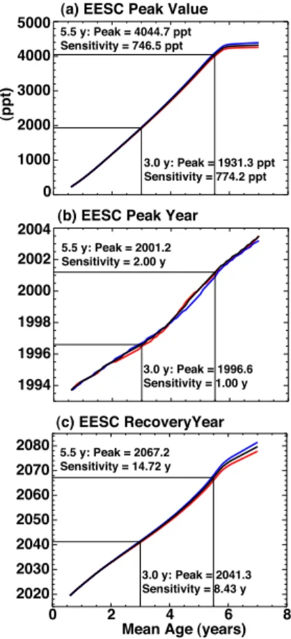
implies that the stratospheric EESC level was lower in 1980. Therefore, the return to that lower level will take longer. The 3-year mean age implies an EESC recovery near 2041, while the older 5.5-year mean age implies a recovery near 2067. Figure6a dis-plays the peak EESC value versus age-of-air (black). The EESC peak is very sensitive to mean age-of-air, and increases from zero for a zero mean age to 4045 ppt for a

15

5.5-year mean age. This increase results from the competition between the fractional release, which results in more liberated chlorine and bromine as the age increases, and the greater flattening of the peak arising from the larger age spectrum width as the age increases. For mean ages above about 5.8 years, nearly all of the organic species have been degraded, so little additional chlorine or bromine is available for release. For

20

a 5.8-year age, Fig.6b shows the peak year versus mean age-of-air (black). The peak year varies almost linearly with age. Each additional year of age results in approxi-mately a 1.0- to 1.5-year increase in the peak year. The asymmetries in the EESC time series and the consideration of the age spectrum are the reasons the increase is not exactly 1.0 year.

25

Recovery is very sensitive to mean age-of-air (Newman et al., 2006). Figure 6c shows the recovery year versus mean age-of-air (black). Each additional year of age results in approximately a 10-year delay of the recovery. This large recovery sensitivity to mean age-of-air can be understood by examining Fig.4c. Because of the large age,

(14)

ACPD

Full Screen / Esc

EGU relative EESC for a 5.5-year mean age (appropriate to the Antarctic polar vortex)

con-tinues to grow during the 1995–2001 period, reaching a value that is nearly double its 1980 value. The relative EESC for a 3-year mean age (appropriate for the midlatitudes) only increases an additional 66% from 1980 to 1996. Because the decay rates (post 2001) for these relative EESC curves are similar, the EESC for 3-year air recovers

5

much earlier than for 5.5-year air.

5.2 Sensitivity to width

In our calculations of the age spectra, we have assumed that the age spectrum width is half of the mean age-of-air (∆ = Γ/2). This is used in all of Fig.1through Fig.5. We test the sensitivity to the spectral width by applying simple increases and decreases

10

to the width. This has no effect on the fractional release values used because they are determined from the mean age alone. In Fig.6, the spectral width has been both increased (red) and decreased (blue) by 30%. For example, the 5.5-year age spectrum width has been varied from 1.9 y to 3.6 y. The largest differences for the peak EESC value and recovery year occur for the largest ages. However, even then the values

15

are not very sensitive to variations in ∆ for any of the three metrics. For a 5.5-year mean age, the peak value decreases by only 46 ppt (1.1% of the 4045 ppt value) with a 30% increase of the spectrum width of 0.8 y. The peak year and the recovery year also demonstrate small variations for large width variations. For a 5.5-year mean age of air, increasing the width by 30% advances (or hastens) the date of recovery by 1.1 y

20

(2067.2 to 2066.1), while decreasing the width by 30% delays the recovery by 1.0 y to 2068.2. In summary, in contrast to variations in mean age the EESC is only moderately sensitive to variations in the spectrum width.

5.3 Sensitivity toα

Because the bromine catalytic cycle is more efficient for ozone loss than the chlorine

25

(15)

ef-ACPD

Full Screen / Esc

EGU ficiency. Model estimates of α show variations with time, altitude, and latitude (e.g.,

Daniel et al.,1995). Inspection of Fig. 5 ofDaniel et al.(1995) shows a variation ofα

from a minimum of about 25 at the equator to a maximum of 65 at 90◦S. Hence, while we have adopted the WMO (2007) value, it is important to note that different values should probably be used for the midlatitudes and polar regions.

5

Figure7repeats the EESC from Fig.5for both a 3-year mean age (lower black) and a 5.5-year mean age-of-air (upper black). We also show the EESC for α=40 (blue)

and_{α=80 (red). From Fig.} 3b, we see that Br_y peaks at approximately 9 ppt for a 3-year mean age. For the 3-3-year mean age-of-air, an increase or decrease ofα by 20

will increase or decrease EESC by 172 ppt. For a 5.5-year mean age-of-air EESC is

10

changed by 304 ppt for a change inα by 20. Because Bry peaks later than Cly (see Fig.3) an increase ofα, which increases the relative importance of Bry, thereby delays the peak year of the maximum EESC. However, this shift is small. Increasingα from

60 to 80 increases the peak year from 2001.2 to 2001.5. The EESC recovery year is also impacted in a minor way by an increase or decrease ofα. Increasing α from 60 to 15

80 delays the 5.5-year mean age recovery year from 2067.2 to 2068.0, and increases the 3-year mean age recovery year from 2041.3 to 2042.5. In summary,α is relatively

important to the peak value of EESC, but is relatively unimportant for the EESC peak year or the EESC recovery year.

It is important to realize that a change ofα does not imply the extent to which the 20

Cly or Bry destruction of stratospheric ozone is changing. Rather, it only provides information concerning how the relative efficiency of Cly is changing with respect to Bry for ozone destruction. Hence, while the chlorine and bromine contributions to EESC can be directly related to Cly and Bry, the summed EESC quantity loses this direct relationship because of the introduction of the multiplicative α factor. Danilin

25

et al. (1996) modeled ozone loss in the Antarctic vortex and computed α for a range

of Cly and Bry values. In their calculation, they showed that for a fixed amount of Bry,

α increases as Cly increases, and for fixed Cly, α decreases as Bry increases. We have taken their estimates ofα and calculated α as a function of time for the Cly and

(16)

ACPD

Full Screen / Esc

EGU Br_y values estimated using our age spectra and release rates. Figure7 shows EESC

calculated using these time-varyingα values (magenta) for a mean age of 5.5 y. Their

estimatedα has a value of 43.1 in 1980 and 41.5 in 2067. As is apparent in Fig. 7, this curve is slightly higher than the_{α=40 (blue) curve. The recovery year using the α} values fromDanilin et al.(1996) is 2065.9. Using a fixed value ofα=42.1, the recovery 5

year is 2066.4. Hence, a temporal varyingα value leads to only modest changes in the

recovery year.

5.4 Sensitivity to halogen scenarios

The full EESC time series depends on both the mixing ratio observations (pre-2006) and the future scenario that is estimated from projected chlorine and bromine

emis-10

sions (post 2006). We have estimated the sensitivities of recovery times to variations in scenarios presented byWMO(2007). Figure8displays EESC versus time for three different scenarios. Scenario A1 fromWMO(2007) is shown (black), again repeating our 3-year (lower) and 5.5-year (upper) mean age-of-air results. Also shown are the mean age-of-air results that are derived from scenario Ab (blue) in the previous

as-15

sessment (WMO,2003). There are two main differences between these results. First, between 2005 and 2020, the EESC from scenario A1 falls off faster than the older sce-nario Ab. This results from the downward revision of methyl bromide concentrations. Second, from approximately 2020 to 2080, the EESC for scenario A1 is higher than the older scenario Ab. While methyl bromide has been revised downward, CFC-11, CCl4,

20

Halon 1211, and HCFC-22 have all been revised upward (WMO,2007). The main con-tribution to this increase is the higher levels of HCFC-22 in the 2020 to 2080 period. The change from scenario Ab to A1 leads to a slight delay of recovery from 2039 to 2041.3 for the 3-year mean age and from 2064.3 to 2067.2 for the 5.5-year mean age. While the scenario revision betweenWMO(2003) andWMO(2007) is substantial, the

25

change in recovery between the scenarios is modest.

Figure8also displays EESC versus time for scenario E0 (red), which includes zero future emissions (WMO,2007). While the attainment of zero emissions is highly

(17)

un-ACPD

Full Screen / Esc

EGU likely, it provides a useful theoretical lower limit on future ODS concentrations and a

corresponding limit on recovery. For a 3-year age, the E0 recovery is 2029 as opposed to the baseline case of 2041. For a 5.5-year age, the E0 recovery is 2053 as opposed to the baseline case of 2067.

5.5 Sensitivity to fractional release values

5

The peak EESC value, the year of this peak value, and the recovery year are all depen-dent on the fractional release values of the various species. These sensitivities depend largely on the magnitude of the contribution of the particular halogen species to the to-tal EESC. For example, CFC-115 had a surface mixing ratio of about 9 ppt in 2000, hence it has a small contribution to an overall 1980 EESC level of 2200 ppt (5.5-year

10

mean age). The peak EESC, the peak year, and the recovery year are not strongly impacted by uncertainty in the CFC-115 fractional release values. Table1shows the sensitivity of peak EESC and the recovery year for a 0.10 fractional release variation centered on the assumed value of fractional release. For a 3-year mean age-of-air, CFC-11 has a fractional release of 0.47. For a variation of 0.42 to 0.52 in fractional

15

release, the maximum EESC changes by 79.9 ppt and the recovery date increases by 0.47 y.

Increasing the fractional release values always increases the peak EESC value. The sensitivities of the maximum EESC value in Table1are proportional to the concentra-tion of the particular species, while the sensitivities of the year of recovery are

propor-20

tional to the mixing ratio difference between the value at the time of EESC recovery to the value in 1980. Because the atmospheric concentrations of species such as CFC-11, CFC-12, methyl chloride, and methyl bromide are large, the sensitivity of the peak EESC to release variations is also large.

In contrast to the EESC magnitude, increasing fractional release can cause the

re-25

covery date to be earlier (negative sensitivity) or later (positive sensitivity). A negative sensitivity example comes by increasing the fractional release of methyl chloroform. In-creasingf by 0.1 moves the recovery date for 3-year air 1.37 years earlier from 2041.3

(18)

ACPD

Full Screen / Esc

EGU to 2039.9 (0.58 years earlier for 5.5-year air). This negative sensitivity results from the

methyl chloroform time history. In Fig. 2c, methyl chloroform was relatively large in 1980, peaked in early 1994, and had fallen to zero by 2041. Increasing the fractional release for methyl chloroform by 0.1 increases 1980 EESC but does not change 2041 EESC. The total Cl_y in Fig. 2d shows a recovery line drawn from the 1980 vertical

5

line. Increasing methyl chloroform (via a fractional release increase) increases 1980 EESC without changing 2041 EESC, shifting the recovery to an earlier date. Carbon tetrachloride and methyl bromide have similar negative sensitivities for 3-year-old air.

Most species exhibit a positive increase in recovery date for an increase in fractional release. Again, this increase is sensitive to the mixing ratio difference of the particular

10

species at the time of recovery compared to 1980. Inspection of Fig.2b and Fig.2d shows that CFC-12 makes a large contribution in 1980, 2041, and 2067 to the overall Cly. Increasing the CFC-12 contribution to Cly by increasing the fractional release will push recovery further into the future because the CFC-12 contribution is larger at the time of expected recovery than it was in 1980. For a 3-year age, if the release

15

is increased from 0.18 to 0.28, the recovery year is increased from 2041.3 to 2043.9 (2.58 y).

We estimate the uncertainty in recovery dates using a Monte Carlo approach on the fractional release values by randomly varying all of the fractional release values for those species shown in Table 1. The release values are altered from their standard

20

values by adding variability with a standard deviationσ=0.05. This 0.05 standard

devi-ation is chosen as a nominal uncertainty by inspection of the CFC-11 versus age curve inSchauffler et al.(2003). Fractional release values are constrained to range between 0.0 and 1.0. The uncertainty in fractional release values leads to a moderate uncer-tainty in the year of recovery. For a 3-year mean age, the 95% confidence limits on

25

the 2041.3 recovery date vary from 2036.1 to 2045.1 (_{σ=2.2 y). For a 5.5-year mean} age, the 95% confidence limits on the 2067.2 recovery date are from 2066.0 to 2069.4 (σ=0.86 y).

(19)

ACPD

Full Screen / Esc

EGU prescribed variation in fractional releaseδf_i = f′− f can be theoretically derived from

Eq. (1). EESC′

i(y) − EESCi(y) = niδfiρi(y) is the difference in EESC for a given year

y. Using EESC′

i(1980) = EESC′i(y + δyi) = EESC′i(y) + ∂EESC′i/∂t δyi (from a

Taylor expansion), and noting that EESC_i(y) = EESCi(1980) and that∂EESC/∂t ≈

∂EESC′

i/∂t gives

5

∂EESC/∂t δy = EESC′

i(1980) − EESC′i(y)

= [EESC′

i(1980) − EESCi(1980)]

−[EESC′_i(y) − EESCi(y)]

= niδfiρi(1980) − niδfiρi(y) (5)

Solving forδyi gives

10

δyi = −

δf_in_i[ρ_i(y) − ρi(1980)]

∂EESC/∂t , (6)

A comparison of recovery year sensitivity to individual fractional release values can be seen in Table1. In general, the magnitude of the sensitivity is smaller for a 5.5-year mean age than for a 3-year mean age.

The smaller uncertainty in the recovery for the 5.5-year mean age-of-air results from

15

the larger rate of EESC decreases at the time of recovery (∂EESC/∂t). Inspection

of Fig. 5 reveals that EESC is changing at a rate of about −20 ppt y−1 _{for 5.5-year} air in about 2067, while the decline rate is a about −13 ppt y−1 for 3-year air in about 2041. The sensitivity is inversely proportional to this decline rate, and so the sensitivity decreases as mean age-of-air increases.

20

5.6 Sensitivity to recovery start date

In all figures herein, the recovery dates indicated are determined from the EESC level in 1980. This 1980 value is chosen as a useful mark because the amount of ozone

(20)

ACPD

Full Screen / Esc

EGU depletion at midlatitudes and in the Antarctic vortex was relatively small. While the

choice of a specific year is somewhat arbitrary, 1980 is the year often considered in previous work (WMO,1999,2003,2007) and has been adopted herein for our standard calculations.

The recovery date is very sensitive to this starting date. In spite of the previous

5

justification for the choice of 1980, the ODS level in 1980 should not be considered as the pre-ozone depletion level; for example, for a 3-year mean age, EESC had more than doubled between 1950 and 1980 (Fig.3). EESC increased rapidly over the 1970s (Fig.5), and it is clear fromFarman et al. (1985) that some ozone loss had occurred as early as 1975 over Antarctica. If the start date for ozone loss is set to 1975 rather

10

than 1980 then the recovery is pushed from 2041.3 to 2063.0 for a 3-year mean age and from 2067.2 to 2097.0 for a 5.5-year mean age. Figure9displays the sensitivity to recovery date. A shift of one year changes the recovery by approximately ten years. However, this result does not change the fact that the date corresponding to 1980 EESC levels still represents a time when ozone loss due to ODSs, in the absence of

15

other atmospheric changes, should be relatively small compared to the losses of the past decade or so.

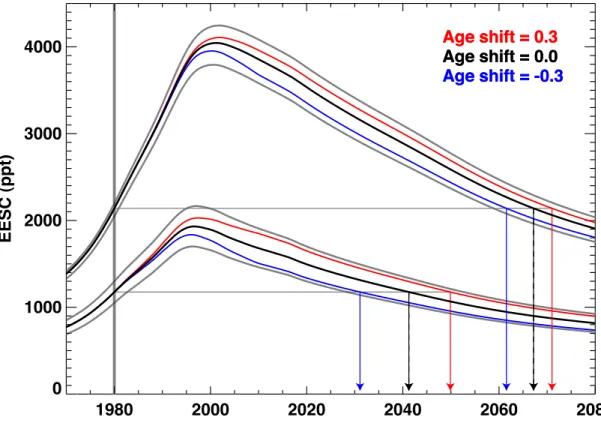
5.7 Sensitivity to temporal changes of age-of-air and fractional release rates

In the above calculations we have assumed that the mean age-of-air is constant in time. However, model simulations suggest that the mean age may decrease with time

20

as a result of an accelerated mean circulation from climate change. Austin and Li (2006) show an age decrease at 60–90◦N and 35 hPa of about 0.15 years per decade. In addition to decreasing mean age, an accelerated circulation changes the fractional release values. A faster circulation will both decrease the age and shift the fractional release values to higher numbers, while a slower circulation has the opposite effect.

25

Hence, we cannot assume that either mean age-of-air or fractional release values are constant in time.

(21)

ACPD

Full Screen / Esc

EGU decreasing and increasing the mean age by 0.3 years over the 1980 to 2010 period.

This change, while significant, is still smaller than the decrease calculated byAustin and Li (2006) for the polar lower stratosphere. To calculate the coherent variation of release rates, we have drawn upon a time series of CFC-11, CFC-12 and mean age-of-air from the Goddard Earth Observing System (GEOS-4) chemistry/climate model

5

(CCM) (Stolarski et al.,2006a). Based upon the GEOS-4 model, we coherently vary all of the fractional release values with mean age by increasing release values by 1% for each 0.1-year change of mean age.

Figure 10 shows EESC for an increase of age from 3.0 y to 3.3 y (lower red) and 5.5 y to 5.8 y (upper red), and a decrease of age from 3.0 y to 2.7 y (lower blue) and

10

from 5.5 y to 5.2 y (upper blue). For the 3-year mean age, the 0.3-year age change substantially alters the EESC behavior and recovery date. Reducing the age from 3.0 y to 2.7 y accelerates recovery from 2041.3 to 2031.1. Shifting the 5.5-year age by 0.3 years has a somewhat smaller effect; reducing the age from 5.5 y to 5.2 y accelerates recovery from 2067.2 to 2061.5.

15

The above large changes in recovery date, at first glance, appear to be inconsistent with the earlier analysis of sensitivity to mean age, where a change of 0.3 y resulted in a 3-year shift in the recovery date (compare with the above 11- to 12-year shift for age decreasing by 0.3 y). As noted earlier from Fig. 4c, the EESC decreases at a relatively regular rate in the period after about 2001 for a constant mean age-of-air. An

20

acceleration of the circulation decreases the age but increases the fractional release values. Overall, the change in the circulation will act to decrease the EESC.

To calculate the overall impact of a temporal shift, we again use the time series of mean age-of-air from the GEOS-4 CCM (Stolarski et al.,2006a). In this CCM run, the mean age-of-air shows decadal variations on the order of 0.1–0.2 y. To simulate this

25

effect, we generate artificial age-of-air time series using the statistical characteristics of the model’s age-of-air time series. In particular, we take detrended polar and mid-latitude time series of age-of-air from model runs extending to 2100, compute a power spectrum from those time series, and fit a power law to those analyzed time series. We

(22)

ACPD

Full Screen / Esc

EGU then add noise to these power law fits using a gamma distribution, and randomly vary

the temporal phase of each frequency over the period from 1950 to 2100. These ran-dom time series of age-of-air lead to EESC variation in both 1980 and at the recovery period. For the 3-year mean age of air EESC the standard uncertainty,σ, in the year

of recovery is 4.4 y, while for the 5.5-year mean age of air_{σ=2.4 y.}

5

5.8 Combined uncertainties

The previous sections discussed EESC sensitivities. In this section we perform Monte Carlo simulations to calculate the recovery date uncertainties assuming future halo-carbon abundances in the A1 scenario ofWMO (2007) are accurate (summarized in Table2). The first row summarizes the uncertainty in the mean age-of-air, Γ. Inspection

10

of Fig. 6 fromAndrews et al.(2001) suggestsσ ≈ 0.3 y. We vary the age with σ=0.3 y

using a Monte Carlo technique in our EESC calculations while holding all other vari-ables fixed, with the exception that fractional releases vary with the mean age. This Monte Carlo technique yields a probability distribution function (PDF) withσ=2.64 y for

3-year old air and_{σ=4.09 y for 5.5-year old air. The 3-year 95% confidence limits for}

15

the 2041.3 recovery are from 2036.1 to 2046.5, while the 5.5-year limits are 2059.2 to 2074.4.

We similarly use the Monte Carlo technique to calculate PDFs for ∆, α, f , and the start date. The uncertainty on ∆ is estimated fromAndrews et al.(2001) andSchoeberl et al. (2005), onα and the start date is fromWMO(2007), onf is fromSchauffler et al.

20

(2003), and on the temporal variations in Γ is from the analysis of the GEOS-4 CCM model output (Stolarski et al.,2006a). In the case of the age temporal variations (Γ(t)+ red noise), we have not coherently adjusted the fractional release values with mean age, such that this variance is an upper limit.

The total uncertainty is calculated by varying all of the factors listed in Table2. For

25

EESC with a 3-year mean age-of-air (recovery in 2041.3), the distribution of recovery dates is somewhat skewed, with 95% confidence limits of 2027.7 and 2048.7. This uncertainty is dominated by our assumption that mean age is a fixed constant. For

(23)

ACPD

Full Screen / Esc

EGU the Antarctic EESC with a 5.5-year mean age-of-air (recovery in 2067.2), the 95%

confidence limits are 2056.3 and 2077.6. This 5.5-year uncertainty is dominated by the uncertainty in value of the mean age.

6 Summary and discussion

EESC is an important quantity for estimating the effect of surface ODS emissions and

5

concentrations on stratospheric chlorine and bromine levels, and can provide insight into peak Cl_y and Br_y levels in the stratosphere and into future ozone recovery. In this paper we have described a reformulation of the technique for estimating EESC. This reformulation uses both fractional release rates that are dependent upon mean age-of-air, and an age spectrum to represent the transport time lag between the

tropo-10

spheric levels of ODSs. In addition to EESC, this reformulation also provides quantita-tive estimates of Cly, Bry, and total inorganic fluorine that are dependent on the mean age-of-air.

Using this new formulation we have estimated new ODS recovery dates for the strato-sphere. We estimate, given the future halocarbon abundances projected in A1 ofWMO

15

(2007), that midlatitude recovery will occur in 2041 while the Antarctic region will re-cover in 2067. Midlatitude air is characterized by an age-of-air of approximately 3 years, while Antarctic lower stratospheric air has a mean age of approximately 5.5 years. We have followedWMO(2007) by using a bromine scaling factor of 60 and their scenario A1. This contrasts with theWMO (2007) estimates of 2048.6 and 2064.7. The

dif-20

ferences in these estimates are primarily due to differences in the fractional release values of a few ODSs. The 95% confidence limits for the midlatitude 2041 recovery are 2027.7 and 2048.7, while the Antarctic limits are 2056.3 and 2077.6.

Newman et al.(2006) estimated that the ozone hole’s area would fully recover (de-crease to a zero size) by 2068. This estimate was based upon a 5.5-year mean

age-25

of-air, scenario Ab ofWMO(2003), and an empirical estimate that the ozone hole had an initial zero size in mid-1979, not 1980. In that study, they confined the observations

(24)

ACPD

Full Screen / Esc

EGU to the vortex where age-of-air ought to be relatively uniform and a constant value as a

function of time. Using the new Scenario A1 fromWMO(2007) we estimate that the ozone hole’s recovery date shifts by 2 years to 2070.

We have also explored the sensitivity of EESC to a number of parameters. These parameters include mean age-of-air, age spectrum width, bromine efficiency for ozone

5

destruction versus chlorine, fractional release, starting date for ODS losses, and tem-poral changes of mean age-of-air and fractional release values. The recovery dates for EESC are primarily dependent upon the mean age-of-air and trends in the mean age-of-air. For example, the Antarctic EESC recovers at a later date than the midlati-tude EESC because the air in the Antarctic stratosphere is older. A temporal trend in

10

mean age with a coherent variation of release rates also can impact recovery strongly. Austin and Li(2006) estimated that Arctic stratospheric air (60–90◦N, 35 hPa) would become younger by approximately 0.5 y between 1980 and 2040, while upper strato-spheric tropical air (20◦_S–20◦_{N, 1.3 hPa) would become younger by 0.8 y. If air in} midlatitude stratosphere becomes younger by 0.3 y, we estimate that recovery will be

15

advanced from 2041.3 to 2031.1.

The strong dependence of EESC on mean age-of-air exposes a crucial assumption that underlies many trend studies and future EESC projections: viz., mean age-of-air and fractional release values are constant over the ozone data record. A shift in mean age can significantly impact interpretation of ozone trends and EESC values.

20

For a 3-year mean age, a ±0.3 year shift in mean age results in a ±9 year shift in recovery to 1980 values and nearly a 230 ppt (12%) change in the peak EESC value. In ozone trend studies, it has been assumed that EESC has a fixed shift with respect to the tropospheric values (typically 3 years). Changes in the circulation will cause both changes in the advection of ozone and age-of-air, and therefore the EESC of the lower

25

stratosphere. EESC variations resulting from age-of-air variation have the potential to lead to large variations of ozone.

The analysis of ozone trends also requires a careful consideration of sampling issues to insure that the fractional chlorine and bromine release values can be accurately

(25)

ACPD

Full Screen / Esc

EGU parameterized. This can be accomplished by ensuring that the mean age-of-air is

either large (greater than 5.8 years) or is relatively constant over the ozone observation record. Sampling of ozone near the edge of the polar vortex is particularly susceptible to such a problem because of the large gradient of age-of-air at the polar vortex edge. Great caution must be exercised in interpreting ozone trends because of the variation

5

of age-of-air spatially and over the observation time period.

The EESC estimates have proven extremely useful for estimating recovery and for exploring various emission scenarios. However, the use of EESC is limited by the assumptions that underlie the calculations. First, estimates of fractional release rates and mean age-of-air are largely calculated from midlatitude and Arctic observations

10

in the lower stratosphere during the last 15 years. Models show that release rates are also a function of altitude and that the mean ages in the stratosphere may be changing. Second, we have assumed that the fractional release observationally derived functions are also fixed in time. This assumption cannot be strictly justified because of both circulation and chemistry changes in the future. Finally, while EESC is a convenient

15

parameter for recovery estimates, it is not equivalent to ozone, and it does not include the fully interactive elements of a coupled climate/chemistry model.

Acknowledgements. This research was funded under the NASA Atmospheric Chemistry,

Mod-eling, and Analysis Program. The comments and discussions with A. Douglass, S. Montza, and R. Stolarski were also extremely helpful.

20

References

Andrews, A. E., Boering, K. A., Daube, B. C., Wofsy, S. C., Loewenstein, M., Jost, H., Podolske, J. R., Webster, C. R., Herman, R. L., Scott, D. C., Flesch, G. J., Moyer, E. J., Elkins, J. W., Dutton, G. S., Hurst, D. F., Moore, F. L., Ray, E. A., Romashkin, P. A., and Strahan, S. E.: Mean ages of stratospheric air derived from in situ observations of CO₂, CH₄, and N₂O, J. 25

Geophys. Res., 106(D23), 32 295–32 314, doi:10.1029/2001JD000465, 2001. 3969,3983 Austin, J. and Li, F.: On the relationship between the strength of the

(26)

Brewer-ACPD

Full Screen / Esc

EGU

Dobson circulation and the age of stratospheric air, Geophys. Res. Lett., 33, L17807, doi:10.1029/2006GL026867, 2006. 3981,3982,3985

Daniel, J. S., Solomon, S., and Albritton, D. L.: On the evaluation of halocarbon ra-diative forcing and global warming potentials, J. Geophys. Res., 100(D1), 1271–1285, doi:10.1029/94JD02516, 1995. 3965,3967,3976

5

Danilin, M. Y., Sze, N.-D., Ko, M. K., Rodriguez, J. M., and Prather, M. J.: Bromine-chlorine coupling in the Antarctic ozone hole, Geophys. Res. Lett., 23(2), 153–156, doi:10.1029/95GL03783, 1996. 3976,3977,3997

Dhomse, S., Weber, M., Wohltmann, I., Rex, M., and Burrows, J. P.: On the possible causes of recent increases in northern hemispheric total ozone from a statistical analysis of satellite 10

data from 1979 to 2003, Atmos. Chem. Phys., 6, 1165–1180, 2006,

http://www.atmos-chem-phys.net/6/1165/2006/. 3966

Farman, J. C., Gardiner, B. G., and Shanklin, J. D.: Large losses of total ozone in Antarctica reveal seasonal ClO_x/NOxinteraction, Nature, 315, 207–210, doi:10.1038/315207a0, 1985. 3981

15

Guillas, S., Tiao, G. C., Wuebbles, D. J., and Zubrow, A.: Statistical diagnostic and correction of a chemistry-transport model for the prediction of total column ozone, Atmos. Chem. Phys., 6, 525–537, 2006,

http://www.atmos-chem-phys.net/6/525/2006/. 3966

Montzka, S. A., Butler, J. H., Myers, R. C., Thompson, T. M., Swanson, T. H., Clarke, A. D., 20

Lock, L. T., and Elkins, J. W.: Decline in the tropospheric abundance of halogen from halocarbons: Implications for stratospheric ozone depletion, Science, 272, 1318–1322, doi:10.1126/science.272.5266.1318, 1996. 3966,3967

Newchurch, M. J., Yang, E.-S., Cunnold, D. M., Reinsel, G. C., Zawodny, J. M., , and Russel, III, J. M.: Evidence for slowdown in stratospheric ozone loss: First stage of ozone recovery, 25

J. Geophys. Res., 108(D16), 4507, doi:10.1029/2003JD003471, 2003. 3966

Newman, P. A., Nash, E. R., Kawa, S. R., Montzka, S. A., and Schauffler, S. M.: When will the Antarctic ozone hole recover?, Geophys. Res. Lett., 33, L12814, doi:10.1029/2005GL025232, 2006. 3965,3966,3968,3969,3972,3973,3974,3984 Schauffler, S. M., Atlas, E. L., Donnelly, S. G., Andrews, A., Montzka, S. A., Elkins, J. W., Hurst, 30

D. F., Romashkin, P. A., Dutton, G. S., and Stroud, V.: Chlorine budget and partitioning during the Stratospheric Aerosol and Gas Experiment (SAGE) III Ozone Loss and Validation Experiment (SOLVE), J. Geophys. Res., 108(D5), 4173, doi:10.1029/2001JD002040, 2003.

(27)

ACPD

Full Screen / Esc

EGU

3968,3970,3972,3973,3979,3983

Schoeberl, M. R., Douglass, A. R., Polansky, B., Boone, C., Walker, K. A., and Bernath, P.: Estimation of stratospheric age spectrum from chemical tracers, J. Geophys. Res., 110, D21303, doi:10.1029/2005JD006125, 2005. 3969,3983

Sarma, K. M., and Bankobeza, G. M.: The Montreal protocol on substances that deplete the 5

ozone layer, United Nations Environment Programme, Nairobi, Kenya, 2000. 3964

Solomon, S. and Albritton, D.: Time-dependent ozone depletion potentials for short- and long-term forecasts, Nature, 357, 33–37, doi:10.1038/357033a0, 1992. 3968,3973

Stolarski, R. S., Douglass, A. R., Gupta, M., Newman, P. A., Pawson, S., Schoeberl, M. R., and Nielsen, J. E.: An ozone increase in the Antarctic summer stratosphere: A dynamical 10

response to the ozone hole, Geophys. Res. Lett., 33, L21805, doi:10.1029/2006GL026820, 2006a.3982,3983

Stolarski, R. S., Douglass, A. R., Steenrod, S., and Pawson, S.: Trends in stratospheric ozone: Lessons learned from a 3D chemical transport model, J. Atmos. Sci., 63, 1028– 1041, doi:10.1175/JAS3650.1, 2006b. 3966

15

Waugh, D. W. and Hall, T. M.: Age of stratospheric air: Theory, observations, and models, Rev. Geophys., 40(4), 1010, doi:10.1029/2000RG000101, 2002.3969

World Meteorological Organization: Scientific assessment of ozone depletion: 1994, Global Ozone Research and Monitoring Project–Report No. 37, Geneva, 1995.3965,3967,3972 World Meteorological Organization: Scientific assessment of ozone depletion: 1998, Global 20

Ozone Research and Monitoring Project–Report No. 44, Geneva, 1999. 3965,3967,3972, 3981

World Meteorological Organization: Scientific assessment of ozone depletion: 2002, Global Ozone Research and Monitoring Project–Report No. 47, Geneva, 2003. 3965,3967,3968, 3972,3973,3977,3981,3984,3998

25

World Meteorological Organization: Scientific assessment of ozone depletion: 2006, Global Ozone Research and Monitoring Project–Report No. 50, Geneva, 2007. 3964,3965,3966,

3967, 3968, 3969, 3970, 3972, 3973, 3976, 3977, 3981, 3983, 3984, 3985, 3989, 3991,

3994,3998

690

Yang, E.-S., Cunnold, D. M., Newchurch, M. J., and Salawitch, R. J.: Change in ozone trends at southern high latitudes, Geophys. Res. Lett., 32, L12812, doi:10.1029/2004GL022296, 2005.

(28)

ACPD

Full Screen / Esc

EGU

Table 1. Fractional release values for all 16 species used in this study for 3-year and 5.5-year

mean age-of-air. ρ_{i ,entry}is the mean surface mixing in 2000 (WMO,2007). Stratospheric life-times that are significantly different than atmospheric lifelife-times are listed. Atmospheric lifelife-times are fromWMO (2007) and stratospheric lifetimes are from C. Jackman (private communica-tion). The sensitivity of the peak EESC value and the recovery year, relative to 1980 EESC values, are for a change inf of 0.10 about the indicated value.

Species Formula ρi ,entry Lifetime Γ = 3 y Γ = 5.5 y

atm. strat. f Peak Recovery f Peak Recovery

EESC year EESC year

ppt y y ppt y ppt y CFC-11 CCl₃F 262.6 45 0.47 79.9 0.47 0.99 78.8 −0.07 CFC-12 CCl₂F₂ 538.0 100 0.23 102.0 2.59 0.86 103.2 1.21 CFC-113 CCl2FCClF2 82.3 85 0.29 24.1 0.91 0.90 23.9 0.42 CFC-114 CClF₂CClF₂ 17.0 300 0.12 3.3 0.09 0.40 3.3 0.05 CFC-115 CClFCF3 8.73 1700 0.04 0.7 0.06 0.15 0.8 0.04 Carbon CCl₄ 98.8 26 0.56 41.5 −1.77 1.00 40.7 −1.37 tetrachloride Methyl CH3CCl3 49.9 5 49 0.67 35.3 −1.29 0.99 26.8 -0.58 chloroform HCFC-22 CHClF₂ 139.8 12 288 0.13 10.6 2.36 0.41 11.7 0.33 HCFC-141b CH3CCl2F 11.9 9.3 0.08 0.3 0.40 0.90 1.1 0.12 HCFC-142b CH₃CClF₂ 11.6 17.9 0.01 0.5 0.06 0.29 0.7 0.01 Halon-1211 CBrClF₂ 4.0 16 0.62 18.7 0.61 1.00 20.5 0.10 Halon-1202 CBr2F2 0.05 2.9 0.62 0.4 −0.01 1.00 0.5 0.00 Halon-1301 CBrF₃ 2.7 65 0.28 12.8 1.19 0.80 14.0 0.57 Halon-2402 CBrF₂CBrF₂ 0.41 20 0.65 4.7 0.02 1.00 4.8 _−0.01 Methyl CH3Br 8.9 0.7 49 0.60 55.8 −0.51 0.99 55.0 -0.27 bromide Methyl CH₃Cl 550.0 1 85 0.44 55.0 0.02 0.91 55.0 0.03 chloride

(29)

ACPD

Full Screen / Esc

EGU

Table 2. Estimated uncertainties for recovery dates with 3-year and 5.5-year mean

age-of-air. The lower and upper values are of the recovery year for each side of the two-sided 95% confidence limits, based on the prescribed uncertainties. The years in the header are the standard recovery years corresponding to the mean age-of-air.

Parameter Prescribed uncertainty Γ = 3 y (2041.3) Γ = 5.5 y (2067.2)

σ Lower Upper σ Lower Upper

y y y y y y Mean age (Γ) ±0.3 y 2.64 2036.1 2046.5 4.09 2059.2 2074.4 Width (∆) Γ/2±30% 0.29 2040.6 2041.7 1.01 2064.9 2068.8 α 60±15 1.06 2038.9 2043.1 0.65 2065.8 2068.4 Fractional release (f ) ±5% 2.23 2036.8 2045.4 0.88 2065.9 2069.4 Start date 1980±0.5 y 2.10 2037.2 2045.4 2.48 2062.5 2072.2 Γ(t)+red noise ≈0.3 y 4.36 2032.3 2048.7 1.99 2063.4 2071.0 Total 6.28 2027.7 2052.2 5.50 2056.3 2077.6

(30)

ACPD

Full Screen / Esc

EGU

Fig. 1. CFC-11 as a function of year from scenario A1 ofWMO (2007). The CFC-11 values have been multiplied by 3 to account for its 3 chlorine atoms. The black curve displays the surface concentration. The dashed red and blue curves show these CFC-11 values after an application of a 3-year age spectrum and a 5.5-year age spectrum, respectively. The solid red curve shows the CFC-11 contribution to Cl_yafter applying a 47% fractional release value to the dashed red curve.

(31)

ACPD

Full Screen / Esc

Printer-friendly Version Interactive Discussion EGU 0 200 400 600 800 1000 (ppt) 0 200 400 600 800 1000 1200 (ppt) 1950 2000 2050 2100 0 100 200 300 400 (ppt) 1950 2000 2050 2100 0 500 1000 1500 (ppt) (a) CFC-11 (b) CFC-12 (c) CH3CCl3 (d) Cly HCFC-22 CFC-113 CH₃CCl₃ CCl4 CFC-12 CFC-11 CH₃Cl

Fig. 2. Chlorine species as a function of year for (a) CFC-11 (as in Figure 1), (b) CFC-12,

and (c) methyl chloroform (CH₃CCl₃). The black curve represents the surface chlorine for each species (i.e., surface measurement scaled by the number of chlorine atoms), filled color curves (dashed lines) represent the chlorine concentrations with fractional release for a 3-year (5.5 year) mean age-of-air. (d) Cl_y as a function of year for a 3-year mean age-of-air. The filled color curves represent the summed contributions of each species to Cl_y. The gray vertical line indicates the reference year of 1980.

(32)

ACPD

Full Screen / Esc

EGU

HALON-2402

HCFC-22

(d) EESC (5.5-year mean age) 0 500 1000 1500 (ppt) 0 2 4 6 8 10 (ppt) 1950 2000 2050 2100 0 500 1000 1500 2000 (ppt) 1950 2000 2050 2100 0 1000 2000 3000 4000 (ppt)

(b) Bry (3-year mean age) (a) Cly (3-year mean age)

(c) EESC (3-year mean age)

HCFC-22 CFC-113 CH3CCl3 CCl4 CFC-12 CFC-11 CH3Cl HALON-2402 HALON-1301 HALON-1211 CH3BR HCFC-141b HCFC-22 HALON-1301 CFC-113 CH3CCl3 HALON-1211 CCl4 CFC-12 CFC-11 CH3Cl CH3Br HALON-1301 CFC-113 CH3CCl3 HALON-1211 CCl4 CFC-12 CFC-11 CH3Cl CH3BR

Fig. 3. (a) Inorganic chlorine, (b) inorganic bromine, and (c) EESC versus time for a 3-year

mean age-of-air. (d) EESC versus time for a 5.5-year mean age-of-air. The filled color curves represent the summed contributions of each species to the total. Although all species are included in the total, the species indicated ate the only ones large enough to be visible. The gray vertical line indicates the reference year of 1980. The black horizontal and vertical lines indicate the recovery date of EESC to 1980 values.