HAL Id: hal-03254861
https://hal.umontpellier.fr/hal-03254861
Submitted on 9 Jun 2021
HAL is a multi-disciplinary open access
archive for the deposit and dissemination of
sci-entific research documents, whether they are
pub-lished or not. The documents may come from
teaching and research institutions in France or
abroad, or from public or private research centers.
L’archive ouverte pluridisciplinaire HAL, est
destinée au dépôt et à la diffusion de documents
scientifiques de niveau recherche, publiés ou non,
émanant des établissements d’enseignement et de
recherche français ou étrangers, des laboratoires
publics ou privés.
Water Resources in Côte d’Ivoire Using RCP 4.5 and
RCP 8.5 Scenarios: Case of the Aghien Lagoon
Wa N’dri, Séverin Pistre, Jean Jourda, Kan Kouamé
To cite this version:
Wa N’dri, Séverin Pistre, Jean Jourda, Kan Kouamé. Application of a Deterministic Distributed
Hydrological Model for Estimating Impact of Climate Change on Water Resources in Côte d’Ivoire
Using RCP 4.5 and RCP 8.5 Scenarios: Case of the Aghien Lagoon. Dr. Mustafa Turkmen; Dr.
Kwong Fai Andrew Lo. International Research in Environment, Geography and Earth Science Vol.
9, 9, Book Publisher International (a part of SCIENCEDOMAIN International), pp.129 - 153, 2021,
978-93-91215-91-0. �10.9734/bpi/ireges/v9/5512d�. �hal-03254861�
_____________________________________________________________________________________________________
1Laboratory of Sciences and Techniques of Water and Environment, Felix Houphouet-Boigny University of Cocody-Abidjan,
Abidjan, Côte d’Ivoire.
2HSM, University of Montpellier, CNRS, IRD, Montpellier, France.
Application of a Deterministic Distributed
Hydrological Model for Estimating Impact of Climate
Change on Water Resources in Côte d’Ivoire Using
RCP 4.5 and RCP 8.5 Scenarios: Case of the Aghien
Lagoon
Wa Kouakou Charles N’Dri
1,2, Séverin Pistre
2*, Jean Patrice Jourda
1and Kan Jean Kouamé
1DOI:10.9734/bpi/ireges/v9/5512D
ABSTRACT
This work aims to evaluate the impact of climate change on the quantitative availability of the Aghien lagoon located in the north of the Abidjan district in Côte d'Ivoire. In first step, the semi-distributed
SWAT (Soil and Water Assessment Tools) based physical model [1] was calibrated and validated at the monthly time step over the period 1960-1981, in the Mé watershed where flow rates data are available. SWAT was then applied on the watershed of the lagoon of Aghien which is ungauged but for which the challenges are considerable for the drinking water supply of the Abidjanese population. In a second step, the gross outputs (precipitation, temperatures) of six climate models of the CORDEX-Africa project under the "Representative Concentration Pathways" (RCP 4.5 and RCP 8.5) scenarios were corrected using the delta method. These corrected outputs were used at the SWAT model input to project the impact of climate change on the flow of the Aghien lagoon for horizons 2040 (2035-2056), 2060 (2057-2078) and 2080 (2079-2100). The projections made on these different horizons were compared with the simulated flow over the period 1960-1981. The results show a sensible decrease in the annual flow of the Aghien lagoon compared to the reference period (1960-1981). Under the medium assumption (RCP 4.5), the models predict a decrease in the annual discharge almost 10% on average. Under the pessimistic hypothesis (RCP 8.5), the average annual discharge should decrease by more than 17%. On a monthly basis, flows in August and September would increase by more than 80% and those in October and November would increase by more than 20% in both RCP scenarios.
Keywords: Abidjan; climate change; Côte d'Ivoire; Aghien lagoon; SWAT.
1. INTRODUCTION
Management and water supply remains a major challenge for the Ivorian government. At present, the water needs of the Ivorian populations have increased, in particular those of the autonomous district of Abidjan. A deficit of 58 million m3 / year must be mobilized to meet the water needs of this population [2]. With a view to filling the water deficit in the economic capital Abidjan, it was decided to operate the Aghien lagoon located north of this city.
However, this resource could be impacted by climate change that influences the water balance by altering evapotranspiration rate, temperature, and precipitation [2]. Change of these hydrological
variables will have a negative impact on the availability of water resources in West Africa [3,4] as well as in the rest of the world. Water resources of Côte d'Ivoire, a country in West Africa, will not escape the consequences of this phenomenon caused by the increase of greenhouse gases in the atmosphere. Indeed, studies have shown that the flow rates of some main rivers, in particular, the flows of the Bandama and Sassandra rivers will decrease during the 21st century [5,6]. What would be the case for the Aghien lagoon? For a better understanding of the effects of climate change on the future quantitative availability of this lagoon, the Soil and Water Assessment Tools (SWAT) hydrological model was applied to its basin to simulate the flow over the periods 1960-1981, 2035-2056 (horizon 2040), 2057-2078 (horizon 2060) and 2079-2100 (horizon 2080). The robustness of the SWAT model to the flow in Ivorian context has already been demonstrated simulate on the basin of Buyo [7] and of Taabo [8].
2. STUDY AREA
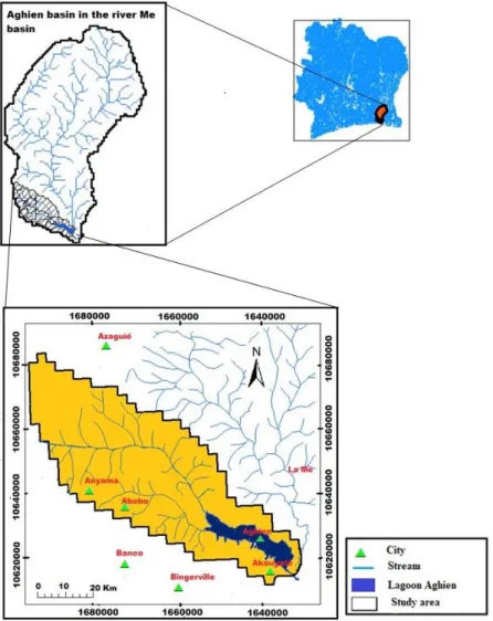
The Aghien basin is located in the southeastern part in Côte d'Ivoire, in the north of economical capital Abidjan. It is a subwatershed of the Mé River basin. The basin area of this river is 4140 km2 (Fig. 1). The Aghien basin has a surface area of approximately365 km2 and lies between 3˚49’ and 3˚58’ W longitude and 5˚21’ and 5˚28’ N latitude. The main tributaries of lagoon Aghien are the Mé, Djbi and Bété rivers.
The Aghien area belongs to the equatorial transition climate. It is characterized by two wet periods (May to July and October to November) and two dry periods (December to April and August to September). The average annual rainfall of the study area is about 1500 mm and average annual air temperature range from 23 to 28, 5°C. The vegetation on the borders of the Aghien lagoon is mainly dominated by swamp forest composed of mangroves and bamboos. This vegetation plays an important role in the stability of the lagoon environment. It acts as a buffer zone by preventing nutrients and sediments from being discharged into the Aghien lagoon and ensures wildlife habitat.
3. MATERIALS AND METHODS
3.1 Materials
3.1.1 Digital elevation model (DEM) data
The digital elevation model (DEM) was downloaded from the shuttle radar topography mission (STRM) website (http://srtm.csi.cgiar.org/SELECTION/inputCoord.asp). It allowed to delineate the watershed, the sub-basins and to calculate slopes and to extract stream network.
3.1.2 Land use data
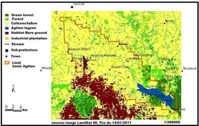
The Aghien Lagoon Basin land cover map (Fig. 2) made from Land SAT Oli-Tirs image under Envi 5.1 (Exelis/envi5.1/help/ENVIHelp.htm# Tutorials, 2013) software was used. It dates from January 2017.
Fig. 2. Aghien Lagoon Basin Land Cover map and surroundings 3.1.3 Soil map and soil type data
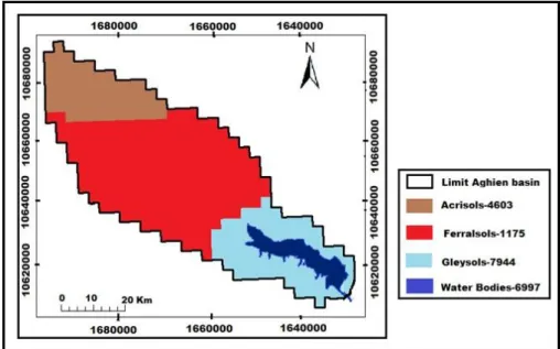
The soil map used in this article is that of FAO (Food and Agriculture Organization of the United Nations), established in 1995 at the scale 1/5000000 for all Africa. It takes into account 5000 soil types and includes the physicochemical properties of soils made by Reynolds et al. (1999) for all Africa. These are essential for the implementation of the SWAT model. The soil data to be integrated into SWAT are: the texture, the available water content, the hydraulic conductivity, the apparent
density, the organic carbon content of the different soil layers. SWAT soil data from the study area were automatically extracted from FAO soil data. To do this, we have established a correspondence between the soil types (moderately and strongly desatured ferralitic soil and hydromorphic soil) of the Aghien lagoon basin and that of the ArcSwat database in which the values of the physicochemical parameters of the soils used by SWAT are recorded. This correspondence allowed to obtain three types of SWAT soils for the Aghien lagoon basin (Fig. 3) which are representative of the types and characteristics of the soil of the zone.
Fig. 3. SWAT Soils Class Map of the Aghien Lagoon Watershed
Fig. 5. Influence area of rainfall stations 3.1.4 Weather data
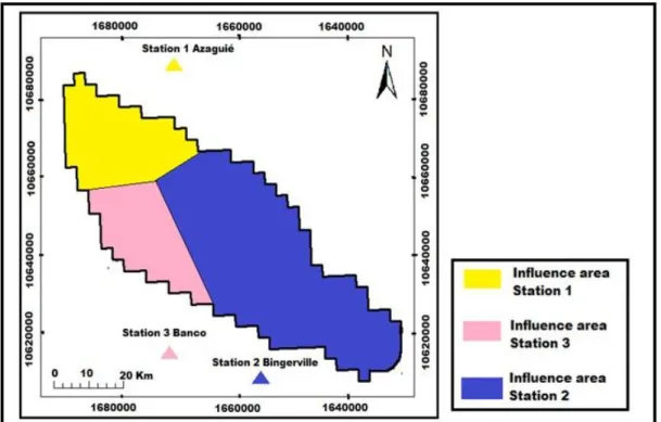
Meteorological data are extracted from the SIEREM database (http://www.hydrosciences.fr/sierem). These data include precipitation and maximum and minimum temperatures at the daily time step and cover the period from 1951 to 1998, which is 47 years. With no data from stations in Aghien Lagoon Basin, we selected SIEREM stations near the Aghien lagoon watershed (Fig. 4) to simulate the flow in this basin. These are the Azaguié, Banco and Bingerville stations.
Fig. 5 shows the area of influence of each station. The different zones of influence were determined by polygon cutting of the Aghien lagoon watershed using Thiessen's improved polygonation method [9]. This method is developed under “extension analyse tools, Proximity, create thiessen polygons of arc-gis 10.2” (http://www.esri.com).
3.1.5 Discharge data
These are daily discharge daily data from the database of Hydrosciences Montpellier (HSM). These data cover the period 1957-1993. It should be noted that they were provided to them by the Water Directorate of Côte d'Ivoire and were recorded at the gauging station of Grand Alépé (Fig. 4). The availability of discharge data is shown in Table 1.
Table 1. Availability of discharge measurements (1957-1993) Date
Station Parameter 1957 to 1974 1975 1976 to 1981 1982 to 1993 Grand Alépé (MÉ) Discharge Available No available Available No available No available: little or no data
3.1.6 Future climate data
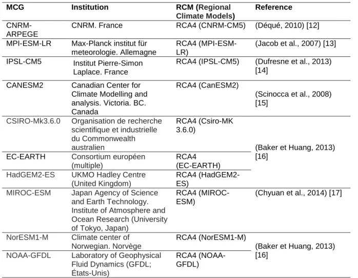
Ten global climate models (GCM) of the CORDEX-AFRICA project under two CMIP5 scenarios (RCP4.5 and RCP 8.5) were considered in this study. These models are presented in Table 2. The variables available in daily under the RCP4.5 and RCP8.5 scenarios are: precipitation, maximum and minimum temperatures, potential evapotranspiration. The outputs of these models cover the period from 1951 to 2100. This period is divided in two: 1951-2005 for historical data and 2006-2100 for future data. RCP 4.5 is a scenario that simulates an increase in the radiative forcing to reach a maximum around 2100 before stabilizing. Under this scenario, greenhouse gas (GES) emissions will peak around 2040, then decline and stabilize around 2080. RCP 4.5 is close to the SRES B1 marker scenario [10]. Contrariwise the RCP 8.5 simulates a constant increase in radiative forcing to reach 8.5 W / m2 in 2100 without reaching a maximum. It is close to the SRES A2 marker scenario [11]. RCP 8.5 is the most pessimistic.
Table 2. List of Ten (10) Global Climate Models (GCMs)
MCG Institution RCM (Regional
Climate Models)
Reference
CNRM-ARPEGE
CNRM. France RCA4 (CNRM-CM5) (Déqué, 2010) [12] MPI-ESM-LR Max-Planck institut für
meteorologie. Allemagne
RCA4 (MPI-ESM-LR)
(Jacob et al., 2007) [13] IPSL-CM5 Institut Pierre-Simon
Laplace. France
RCA4 (IPSL-CM5) (Dufresne et al., 2013) [14]
CANESM2 Canadian Center for Climate Modelling and analysis. Victoria. BC. Canada
RCA4 (CanESM2)
(Scinocca et al., 2008) [15]
CSIRO-Mk3.6.0 Organisation de recherche
scientifique et industrielle du Commonwealth australien RCA4 (Csiro-MK 3.6.0) (Baker et Huang, 2013) [16]
EC-EARTH Consortium européen (multiple)
RCA4 (EC-EARTH)
HadGEM2-ES UKMO Hadley Centre
(United Kingdom)
RCA4 (HadGEM2-ES)
MIROC-ESM Japan Agency of Science
and Earth Technology. Institute of Atmosphere and Ocean Research (University of Tokyo, Japan)
RCA4 (MIROC-ESM)
(Chyuan et al., 2014) [17]
NorESM1-M Climate center of
Norwegian. Norvège
RCA4 (NorESM1-M)
(Baker et Huang, 2013) [16]
NOAA-GFDL Laboratory of Geophysical
Fluid Dynamics (GFDL; États-Unis)
RCA4 (NOAA-GFDL)
3.2 Methods
3.2.1 Evaluation of the performance of climate models
The assessment of the performance of the models to reproduce the two most influential parameters of the hydrological cycle (observed temperature and rainfall), was carried out using the bias method [18]. This method consists in estimating the difference between simulated (Xsim) and observed (Xobs) parameters compared to those observed over the 1960-1981 reference period (eq.1). It is therefore a "relative difference". It makes it possible to evaluate the difference between rainfall and simulated
temperatures at the observations. If the value of the bias is negative then the model underestimates the observed data and if it is positive it overstates the observed data. The interest in evaluating the performance of climate models is to identify the model that best reproduces the interannual variability of cumulative rainfall and temperatures of the Aghien lagoon watershed.
𝐵𝑖𝑎𝑠 =𝑋̅𝑠𝑖𝑚−𝑋̅𝑜𝑏𝑠𝑋̅𝑜𝑏𝑠 (1)
3.2.1.1 Analysis of simulated interannual and seasonal temperatures
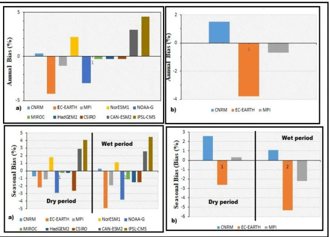
Most models provide reasonably reliable predictions of the annual and seasonal mean temperature of the study basin. Of the 10 global climate models, seven models (CSIRO, hadGEM2, MIROC, NOAA-G, CNRM, Ec-EARTH, and MPI) underestimate the average annual and seasonal temperature of the Bingerville station, while the others (CanESM2, IsplCM5, norESM1) overestimate it (Fig. 6a). At the Azaguié station, only three of the GCMs have temperature and rainfall data. Two (MPI and Ec-EARTH) underestimate the average annual and seasonal temperature while the CNRM model overestimates it (Fig. 6b). The models that give the least biased results are: CNRM, MIROC, HadGEM2, CSIRO (annual) and CNRM, MIROC, HadGEM2 (seasonal) at Bingerville station and MPI, CNRM at Azaguié station. The choice of the performing model was based on the model that overestimates the least and another that underestimates the least.
Fig. 6. Estimation of the bias between observed baseline (1960-1981) and simulated GCM temperatures a) Bingerville station; b) Azaguié station
3.2.1.2 Analysis of simulated interannual and seasonal rainfall
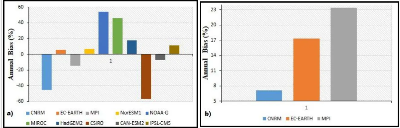
As a first step, a comparison between simulated and observed annual cumulative rainfall was performed. The annual rainfall is overestimated by most GCMs except the CNRM, MPI, CSIRO, IPSL-CM5 models of the Bingerville Station (Fig. 7a). At the Azaguié station, the CNRM, Ec-EARTH and
MPI models also overestimate the annual rainfall (Fig. 7b). The models that best reproduce the annual rainfall are: Ec-EARTH, NorESM1, CanESM2 at Bingerville station and CNRM at Azaguié station.
Fig. 7. Estimation of the bias between observed baseline (1960-1981) and simulated GCM rainfall; a) Bingerville station; b) Azaguié station.
Fig. 8. Estimation of the bias (%) between seasonal total rainfalls observed and simulated over the period 1960-1981; d) Bingerville station; e) Azaguié station
The seasonal cycle simulated by the GCMs clearly shows that the climate models tend to underestimate precipitation during the wet period (May to July and October to November) and to overestimate rainfall during the dry period (December to April and August to September). The total wet period rainfall simulated by the different models shows that the IPSL-CM5, HadGEM2, MIROC models for the Bingerville station (Fig. 8d) and CNRM, MPI, Ec-EARTH for the Azaguié station (Fig. 8e) overall reproduce a structure in phase with the observations. Contrariwise the CNRM, MPI, CSIRO, Ec-EARTH, NorESM1, CanESM2, NOAA-G models (Bingerville station) deviate strongly from the observations. In dry periods, models strongly overestimate total rainfall with the exception of CNRM, CSIRO models from Bingerville station. This large difference between simulated wet season rainfall and simulated dry season rainfall influences the variability of cumulative annual rainfall, as well as the choice of model. The total rainfall of the Aghien lagoon basin is better reproduced by the climate models during the wet period than during the dry period. It is therefore suitable to facilitate the choice of the most efficient model, to compare the observed and simulated data of the wet period only.
The results of the comparison of the biases of the different global climatic models of the CORDEX-AFRIQUE project have shown that a single climate model cannot perform well to reproduce the variability of precipitation for the two stations. There is at least one model capable of reproducing the temporal variability of precipitation for each station and for each time scale.
Since the SWAT hydrological model simulation is carried out at the monthly time step in this study, the global climate models selected are the ones that best simulate the observations at the seasonal scale. Thus, the performing models selected following the analysis of the observed and simulated data are recorded in Table 3 below.
Table 3. List of selected models
Stations Bingerville Azaguié
Parameters Rainfall Temperature Rainfall Temperature
Models IPSL-CM5 HADGEM2 MIROC CNRM MIROC HADGEM2 CNRM MPI EC-EARTH MPI CNRM
Affected of bias more or less importantly, the raw outputs of these models must be accompanied by bias correction methods [19]. Thus, the delta method [20] was required in this study to correct the bias of the selected climate models. This approach corrects two types of distributions:
“additive” disturbances for temperatures
𝑇𝑠𝑐𝑒𝑛, 𝑗, ℎ = 𝑇𝑜𝑏𝑠, 𝑗 + (𝑇𝑠𝑐𝑒𝑛, 𝑚, ℎ − 𝑇𝑟𝑒𝑓, 𝑚) (2)
“multiplicative” disturbances for the precipitations
𝑃𝑠𝑐𝑒𝑛, 𝑗, ℎ = 𝑃𝑜𝑏𝑠, 𝑗 × (𝑃𝑠𝑐𝑒𝑛, 𝑚, ℎ ÷ 𝑃𝑟𝑒𝑓, 𝑚) (3) Tobs,j and Pobs,j are the daily observed temperature and precipitation; Tscen,m,h and Pscen,m,h are the mean monthly temperatures and precipitation simulated by the models over the period of the scenario considered; Tref,m, Pref,m are the mean monthly temperatures and precipitation over the reference period. Tscen,j,h, and Pscen,j,h are the daily temperature and precipitation of the considered time period.
3.2.2 Hydrological Model : SWAT
3.2.2.1 SWAT model description
SWAT “Soil and Water Assessment Tool” is a semi-distributed physically-based model, developed to predict the impact of management practices on water and agricultural chemical yields on a basin scale [1]. It has been developed by researchers at the USDA (United States Department of Agriculture) – Agricultural Research Service [21,22]. SWAT takes into account all the hydrologic cycle, represented in the watershed, so spatialized. The time step used for analysis is the day. SWAT can analyze the impacts of climate, soil, vegetation and agricultural activities on water flow. The basic space unit at SWAT calculations is the Hydrological Response Unit (HRU). It is the result of the combination of a soil type, a land use class and a subwatershed. It is coupled with a GIS(geographic information system) such as ArcView GIS 3.2 or Arcgis 9.x. or Arcgis 10.x from ESRI. This has a double interest. Indeed, the use of a GIS makes it possible both to facilitate the pretreatment of the data to be integrated into the model and also to visualize the results of the simulation. Its implementation requires several input data: digital elevation model (DEM), soil data, weather data, land use data, agricultural practice etc. SWAT, subdivides hydrological modeling of the watershed into two phases [22]: the land phase and routing phase. The land phase is based on soil water balance equation for each day of simulation (4):
𝑆𝑊𝑡= 𝑆𝑊0+ ∑(𝑅𝑑𝑎𝑦 𝑡
𝑖=1
− 𝑄𝑠𝑢𝑟𝑓− 𝐸𝑎− 𝑊𝑠𝑒𝑒𝑝− 𝑄𝑔𝑤)𝑖 (4)
Where: SWt is the final soil water content (mm); SWo is the initial soil water content on day i (mm); t is
day i (mm), Ea is the amount of evaporation on day i (mm); Wseep is the amount of water entering the
vadose zone from the soil profile on day i (mm); Qgw is the amount of return flow on day i (mm).
3.2.2.2 Calibration and validation of SWAT model
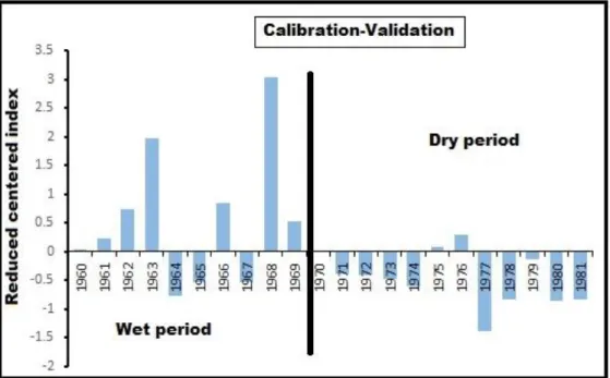
The Aghien lagoon basin is an ungauged basin. However, as shown in Fig. 1, the Aghien lagoon basin is a sub-basin of the Mé basin. They therefore belong to the same geographical area. This geographical proximity is a sufficient indicator of the hydrogeological, climatic and pedological similarity of these two basins [23]. On the basis of this similarity hypothesis, we used the flux data at the daily time step of the Grand Alépé hydrological station on the Mé river to calibrate the SWAT model on this watershed. Thus, the adjusted parameters of the model for the Mé basin have been reintegrated into the model to simulate the flow over the lagoon of Aghien (ungauged) over the period 1960-1981 (baseline period). The calibration procedure requires three main steps. It is first necessary to identify the sensitive parameters (parameters that can influence the performance of the model), then adjust the parameters and finally validate the model over a different period of the calibration phase. Thus, the period 1960-1969 (wet period) was chosen for calibration of the model and validation was carried out on the dry period (1970-1981). Fig. 9 illustrates the periods used for calibration and validation.
Fig. 9. Reduced centered index on precipitation and calibration-validation period retained
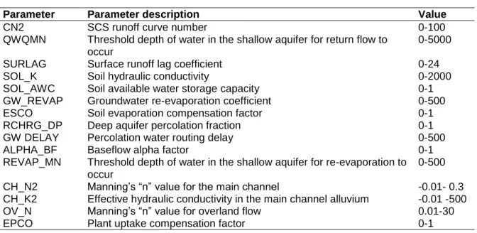
3.3 Sensitivity Analysis of SWAT Model Parameters
SWAT-CUP 5.1.6 was used to analyze the sensitivity of the parameters. Identifying sensitive parameters is the first step in calibrating the SWAT model. It makes it possible to target the parameters that most influence the performance of the model. Thus, it is possible to reduce the number of parameters to be included in the calibration in order to reduce the efforts required in calibration and to increase the probabilities of converging on the performance of the model. It should be noted that in general, the most modified parameters, according to the literature (Table 4), during calibration relate exclusively to the water cycle [24]. This is consistent with the fact that it is primarily controls all other outputs of the model. It is these parameters (the most modified, 15 in number) that will be analyzed to determine their influence on the reproduction of the flow. Thus, the parameters which will have a notable influence on the flow of the Mé river are those which will be adjusted. The optimization process which reflects the sensitivity of the 15 parameters was carried out by two sensitivity analysis methods: The local sensitivity analysis method (One-at-a-time) and the global
sensitivity analysis method. In the local sensitivity analysis method, the principle was to change the value of a single parameter among the 15 to be modified and then to keep constant the values of the other 14 parameters. About 200 iterations were performed for each modification of the parameter. In the overall sensitivity analysis procedure 500 simulations were performed to obtain the most sensitive parameters. The principle consists of assigning values to the parameters and performing a certain number of simulations (500). In both cases, after each simulation, we compared the values of the t-Stat and P-Value coefficients. The t-t-Stat and P-Value coefficients (in SWAT-CUP) identify the most sensitive and least sensitive parameter. A parameter with a larger absolute value of t-Stat is more sensitive. The P-Value gives the importance of sensitivity. When P-Value is close to Zero then the sensitivity of the parameter is important.
Table 4. List of SWAT model parameters used in flow sensitivity analysis
Parameter Parameter description Value
CN2 SCS runoff curve number 0-100 QWQMN Threshold depth of water in the shallow aquifer for return flow to
occur
0-5000 SURLAG Surface runoff lag coefficient 0-24 SOL_K Soil hydraulic conductivity 0-2000 SOL_AWC Soil available water storage capacity 0-1 GW_REVAP Groundwater re-evaporation coefficient 0-500 ESCO Soil evaporation compensation factor 0-1 RCHRG_DP Deep aquifer percolation fraction 0-1 GW DELAY Percolation water routing delay 0-500 ALPHA_BF Baseflow alpha factor 0-1 REVAP_MN Threshold depth of water in the shallow aquifer for re-evaporation to
occur
0-500 CH_N2 Manning’s “n” value for the main channel -0.01- 0.3 CH_K2 Effective hydraulic conductivity in the main channel alluvium -0.01 -500 OV_N Manning’s “n” value for overland flow 0.01-30 EPCO Plant uptake compensation factor 0-1
3.4 Parameter Adjustment
After identifying the sensitive parameters, these parameters must still be adjusted so that they are better suited to the local context. The SUFI-2 optimization algorithm [25] within SWAT-CUP 5.1.6 software was used. The principle consists in varying the value of the sensitive parameter by multiplying all of its values in each URH (R_Relative method) by the same coefficient until obtaining the best value of an objective function (the Nash-Sutcliffe coefficient (NS) and the coefficient of determination R2). The model's Nash - Sutcliffe (NS) coefficient of efficiency is used to assess the predictive power of hydrological models. Its value varies from minus infinity to 1. The closer its value is to 1, the more efficient the model is. A model is considered good if the Nash value is greater than or equal to 0.5 [26]. It is calculated as follows (Equation 5). The coefficient of determination R2 (Equation 6) corresponds to the square of the correlation coefficient which concerns the intensity or the sharpness of the relationship which exists between observed and simulated flows. Its prediction interval ranges from 0 to 1 for a perfect model. A value of R2 greater than 0.5 would indicate a good agreement between the observed and simulated data [27].
(5)
With: Qm : Observed flow, Qs : Simulated flow, 𝑄̅𝑚 : mean of measured flows ; 𝑄̅𝑠 : mean of simulated flows.
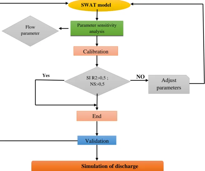
Fig. 10. Diagram of the sensitivity analysis, calibration and validation procedure of the SWAT model
The other measure of the quality of the calibration used in this study is the P-factor (percentage of data in the 95PPU band) and the factor (a measure of the thickness of the 95PPU band). The R-factor quantifies the thickness of the 95PPU and the smaller this number, the smaller the uncertainties and the better the calibration. A desirable value for the R-factor is 1 with a P-factor also close to 1 [28]. Equations 7 and 8 below are used to calculate the P-factor and the R-factor.
(7)
(8) Where QMti, 97,5% et QMti, 2,5% represent the simulated upper and lower limits of the time step ti of the
95PPU, n is the number of observed data points, M refers to the model, ti refers to the step of
SWAT model
Parameter sensitivity analysis Flow parameterCalibration
SI R2>0,5 ; NS>0,5 YesNO
Adjust
parameters
End
calibration
Validation
Simulation of discharge
simulation time, σobs represents the type of data measured and the NQin is the number of flows
observed in the interval 95PPU.
3.5 Validation of SWAT Model Parameters
The principle consists of reinserting into SUFI-2 (Sequential Uncertainty Fitting) the values of the calibrated parameters and the observed flow rates of the validation period to reproduce a second set of observation data. This phase makes it possible to verify the validity of the calibration on all the data and to estimate the predictive nature of the model. Indeed, the calibration was carried out only on part of the data and for it to be accepted, it must be validated globally. The validation was carried out for the flow over the period 1970 to 1981 (calibration over the period 1960-1969). The sensitivity analysis, calibration and validation procedure is shown schematized in Fig. 10.
3.5.1 Climat change simulations
Rainfall and temperature data of the six climate models selected for the RCP 4.5 and RCP 8.5 scenarios allowed simulations of the discharge of the Aghien lagoon. Future simulations of the Aghien lagoon discharge 2040 (2035-2056), 2060 (2057-2078) and 2080 (2079-2100) horizons were compared to the simulations of the baseline period 1960-1981. The comparison between the future simulations and the simulations over the baseline period is made possible because the reproduction of the processes on this period (1960-1981) was validated beforehand, during the calibration / validation phase of the SWAT model. This comparison allowed to analyze the impacts of climate change on the future (quantitative) availability of the Aghien lagoon.
4. RESULTS AND DISCUSSION
4.1 Parameters Sensitivity Analysis
The results of the analysis of sensitive parameters using the local and global sensitivity analysis methods were presented in Table 5 and Fig. 11. Seven parameters were identified as sensitive among the 15 most changed. They are: the parameter CN2, relating to surface runoff, the groundwater level necessary to contribute to the flow QWQMN, SOL_K, the hydraulic conductivity at saturation, the water retention capacity of the soil SOL_AWC, the re-evaporation coefficient of the groundwater GW_REVAP, ESCO the compensation coefficient for evaporation and ALPHA_BF the Baseflow alpha factor. These sensitive parameters are presented in Table 5 and are classified according to their order of importance in terms of their sensitivity. Recall that when a parameter has a larger absolute value of “t-Stat”, it is more sensitive. The “P-Value” gives the importance of sensitivity. When “P-Value” is close to Zero then the sensitivity of the parameter is important. With the global sensitivity analysis method, the most sensitive parameter is the runoff coefficient (CN2) (tStat = -52.31; P-Value = 0.0001) and the least sensitive is the Baseflow alpha factor (ALPHA_BF) (t- Stat = 4.16; P-Value = 0.0007). While with the local sensitivity analysis (one-at-a-time) method, the GW_REVAP parameter is the most sensitive with a “t-Stat value” of -77.18 and a “P-Value” of 0.00001. The least sensitive is ALPHA_BF (t-Stat = -8.16; P-Value = 0.0005). Three parameters were well sensitive in the local analysis method but were not in the global sensitivity analysis method. They are: SURLAG (surface runoff delay), RCHRG_DP (deep water table recharge coefficient) and Gw_DELAY (percolation water routing delay). Finally, five parameters were not sensitive even with the two methods. These are the REVAP_MN (groundwater level necessary to contribute to re-evaporation), CH_K2 (effective hydraulic conductivity in the alluvium of the main channel), CH_N2 (value "n" from Manning for the main channel), OV_N (value "n" from Manning for land flow) and EPCO (soil evaporation compensation factor).
Comparison of sensitive parameters indicates that seven parameters are sensitive as highlighted in Table 5. The most critical parameters in the SWAT model are CN2 (global sensitivity analysis) and GW_REVAP (local sensitivity analysis) with values absolute values of "t-Stat" respectively of 52.32 and 38.21. On Fig. 11, the curve in red shows the variations in the" t-Stat" values of the different parameters for the local sensitivity analysis and the blue one indicates the variations in the "t-Stat" values for the global sensitivity analysis. Our sensitivity analysis results confirm the high sensitivity of
the SWAT model to changes in CN2, groundwater parameters SOL_AWC, GW_REVAP and ALPHA_BF as reported in the study Obuobie [29].
Table 5. Results of the sensitivity analysis of the 15 most modified parameters No Parameters Analysis of global sensitivity Analysis of local sensitivity
t-Stat P-Value rank t-Stat P-Value rank
1 CN2 -52,31 0,0001 1 -38,21 0,0004 3 2 QWQMN 27,58 0,0003 2 11,94 0,0002 5 3 SOL_K -16,66 0,0008 3 42,32 0,0001 2 4 SOL_AWC 12,83 0,0003 4 -7,56 0,0005 6 5 GW_REVAP -9,88 0,0006 5 -77,18 0,0001 1 6 ESCO -6,25 0,0004 6 18,27 0,0002 4 7 ALPHA_BF 4,16 0,0007 7 -8,16 0,0005 7 8 SURLAG -0,242 0,061 8 2,08 0,0077 8 9 RCHRG_DP 0,103 0,607 9 -2,01 0,006 9 10 Gw_DELAY 0,048 0,308 10 1,87 0,0057 10 11 REVAP_MN -0,022 0,118 11 0,0071 0,105 11 12 CH_K2 0,0016 0,0475 12 -0,0044 0,226 12 13 CH_N2 -0,0007 0,0681 13 -0,0011 0,219 13 14 OV_N -0,0002 0,0358 14 0,00005 0,0158 14 15 EPCO 0,00009 0,0455 15 -0,00002 0,0181 15
Fig. 11. Comparison of sensitive parameters of the SWAT model using global and local sensitivity analysis
4.2 Calibration-validation and Assessment of Uncertainties of SWAT Model
A large number of simulations as well as calibration tests were carried out in order to best correlate the simulated flows with the observed flows. Figs. 12, 14, 15 and 16 respectively present the hydrographs observed and simulated over the calibration and validation periods as well as the linear regression curves for the comparison of the flows observed and simulated between 1960 and 1981.
4.2.1 Flow calibration over the period (1960-1969)
Figs. 12 and 13 allow a visual appreciation of the observed and simulated flow hydrographs during calibration over the period 1960 to 1969. We can see in Fig. 12 that the date of occurrence of the flood peaks is generally correct. The observed flow of July 1961 is significantly underestimated by the model. We observe a weak distribution of points (Fig. 13). This indicates good stability in the response
of the model. The result obtained monthly for the Nash criterion (NS) is 0.807 and that of the coefficient of determination R2 is 0.809. These values are acceptable and significantly higher than the guide values of these objective functions (NS, R2). Indeed, the Nash criterion must be greater than 0.5 for a high-performance model and a coefficient of determination greater than 0.5 reflects a good correlation between observed and simulated flows.
4.2.2 Flow validation over the period (1970-1981)
The validation phase ensures that the model accurately reflects the hydrological behavior of the watershed. It was carried out over the period from 1970 to 1981, i.e. 11 years. This phase is important because for any application, the model is used under validation conditions. The value for the Nash criterion (NS) is 0.59 and 0.64 for the coefficient of determination. Figs. 14 and 15 show the hydrographs and the linear regression curve of the observed and simulated monthly flows. We can see in Fig. 14 that the date of occurrence of the flood peaks is correct. However, the flow rates observed are overestimated over the entire validation period. The distribution of points is less good than in calibration as shown in the Fig. 15.
Fig. 12. Monthly observed and simulated water flow in calibration for the Mé basin (1960-1969); Nash= 0. 807
Fig. 13. Correlation between the monthly observed and simulated water flow in calibration for the Mé basin - R2= 0.809
The performances recorded on the coefficient of determination R2 = 0.809 in calibration (1960 to 1969) and 0.64 in validation (1970 to 1981) clearly describe the degree of collinearity between the simulated and measured data. The Nash criteria (NS) in calibration (NS = 0.807) and in validation (NS = 0.59) are generally acceptable even if this coefficient is less satisfactory in validation. According to Saleh et al. [26], Santhi et al. [27] and Bracmourt et al. [30], a Nash coefficient greater than 0.50 is considered acceptable. A slight offset is observed between the curves of the simulated flows and those observed in calibration. This offset is sometimes marked by a temporal lag of the curve of the data observed on the curve of the simulated data and sometimes a time ahead. Indeed, if the curve of the simulated data is behind or ahead of the curve of the data observed temporally and conversely, the coefficient of Nash can decrease in a very sensitive way [31]. Without this offset, the coefficient of Nash would be even better in setting. In validation, the flow rates are overestimated. This overestimation seems to indicate a flow regulation phenomenon which is not considered by the model. In addition, the calibration period is wetter than the validation period. Thus, heavy precipitation over the calibration period can accentuate a poor calibration of the runoff coefficient, which is the most sensitive parameter. This parameter, when it is too high, generates overestimated runoff heights [32], which could justify the overestimation of the flow observed in validation. The modest performance of the SWAT in validation can be explained by the incomplete series of flow data. Indeed, although discharge data are available for the period 1970 to 1981, significant gaps exist. Thus, the month of March of the year 1977 was marked by a total absence of flow data. This could limit the obtaining of good performance of the model in validation (1970-1981). Despite, the shortcomings observed in the flow data series for the reference period (1960 to 1981), the SWAT model shows satisfactory results. In view of these results, the model has therefore demonstrated its robustness in reproducing the flow in the catchment area of the Mé River. This performance of the SWAT model in reproducing the flow has already been demonstrated on the watersheds of: San Joaquin in California [33], Ken in India [34], Burgundy in France [24], Buyo [7] and Taabo [8] in Côte d'Ivoire and in several other basins around the world.
4.2.3 Uncertainties related to flow modeling
As a reminder, P-factor values greater than 0.7 and R-factor values less than 1.5 are recommended to obtain good modeling [35]. Figs. 15 and 16 present the hydrographs of the observed flows and of the 95PPU during calibration and validation. The green color shaded area in Figs. 16 and 17 represents the uncertainty of the SWAT model, while the brown color line represents the time series of observed monthly flows. Thus, the P-factor in calibration is 0.88 and the R-factor is 1.17 while in validation, the P-factor is 0.76 and R-factor is 1.21. The percentage of data within the 95PPU interval is acceptable in both the calibration and validation period.
Fig. 14. Correlation between the monthly observed and simulated water flow in validation for the Mé basin - R2= 0.636
Fig. 15. Hydrogram of observed flows and 95 PPU in calibration (P- factor = 0.88 and R- factor = 1.17)
Fig. 16. Hydrogram of observed flows and 95 PPU in validation (P-factor = 0.75 and R-factor = 1.21)
4.3 Potential
Impacts
of
Climate
Change
on
Precipitation
and
Potential
Evapotranspiration of Aghien Lagoon Basin
4.3.1 Change in Potential Evapotranspiration (PET)
PET shows an overall increasing trend in the 21st century under the RCP 4.5 and RCP 8.5 scenarios. Indeed, trends are becoming more pronounced under both scenarios, towards the end of the 21st century (Table 6), but also a slight stationarity of the PET is observed under the RCP 8.5 scenario between the 2060 and 2080 horizons.
Table 6. Percentage of change in the annual evapotranspiration potential for the different horizons compared the baseline period (1960-1981)
Baseline period 2040 (2035-2056) 2060 (2057-2078) 2080 (2079-2100) Average Variatio n (%) Average Variation (%) Average Variation (%) PET (mm) RCP 4.5 1230,65 1330,28 +8,09 1342,23 +9,06 1369,47 +11,28 RCP 8.5 1358,81 +10,42 1367,95 +11,15 1366,16 +11,05
4.3.2 Change in Rainfall
The evolution of precipitation at different horizons is shown in Fig. 17. The rates of decrease in rainfall are relatively more in RCP 8.5 than RCP 4.5 over the basin. Under RCP 4.5, the rainfall may decrease from 9.06 % on average and under RCP 8.5 rainfall may decrease from 16.96 % on average in future periods. The calculated rates of change are shown in Table 7. The decrease in precipitation is more pronounced towards the end of the century under the two scenarios: 11.80% (horizon 2060), 11.68% (horizon 2080) under the RCP 4.5 scenario and 19.14% (horizon 2060), 19 16% (horizon 2080) under the RCP 8.5 scenario. This rainfall deficit has already been observed in West Africa under the scenarios RCP 4.5 and RCP 8.5 on the watersheds of Senegal and Bandama respectively by Mbaye, [36] and [6]. Also, the work of [7] revealed a decrease of precipitation of 10.27% by 2050 and 14.90% by 2080 on the watershed of the Buyo dam (Côte d’Ivoire) using the SWAT model and the UKMO-HadGEM1 model according to A1B scenario. Given the evolution of these variables (PET and Rainfall), we can expect that the flow of the Aghien lagoon will be impacted by both the decrease in precipitation and the increase in potential evapotranspiration.
Fig. 17. Evolution of annual rainfall compared to the baseline period (1960-1981)
4.4 Potential Impacts of Climate Change on Aghien Lagoon Discharge: Annual and
Seasonal Discharge Evolution
RCP Scenarios 4.5 and 8.5 project a reduction in the annual flow of the lagoon until 2080 (Fig. 18). Under the RCP 4.5 scenario the average annual flow would decrease by 8.33%, 10.02%, and -9.72% respectively over the different horizons (2040, 2060, and 2080). RCP 8.5 scenario forecasts a decrease average flow rate over the different horizon: -16.36% by 2040, -19.15% by 2060 and -19.22. % by 2080.
Fig. 19 (a) and (b) show the seasonal evolution of the lagoon discharge over the different horizons for the RCP 4.5 and RCP 8.5 scenarios compared to the observed flow over the reference period (1960-1981). We note that under both scenarios, the hydrological regime could be disrupted with respect to seasonal flow patterns and the date of occurrence of flood peaks. Indeed, the flood peaks will now appear in August and September instead of June and July over the past period (1960-1981). This situation means that the seasons could move in the 21st century. The RCP 4.5 scenario projects a decrease in the lagoon flow during the long dry season (December to April) of 42% and a decrease during the long rainy season (May to July) of 57%. As for the RCP 8.5 scenario, it predicts a decrease in flow of 44% in the dry season (December to April). It also projects a decrease in the flow of the lagoon of 64% in rainy season (May to July). Both scenarios predict a greater increase in flow (more
than 80%) in August and September during the short dry season and a slight increase in flow (more than 20%) in October and November during the short rainy season.
Fig. 18. Evolution of the annual discharge of the Aghien lagoon under the RCP 4.5 and RCP 8.5 scenario compared to the baseline period (1960-1981)
The discharge of the Aghien lagoon would decrease by an average of 9.42% under the RCP 4.5 scenario and would also decrease by an average of 18.24% under the RCP 8.5 scenario. These results are in agreement with those of [37] in the watersheds of Senegal, Gambia and Sassandra, [38] in the Ouémé river basin in Benin (West Africa), [7] in the watershed of the Buyo dam [39] or [3] in the Comoé river watershed. These authors describe a decrease in stream flows in these different basins, up to about 20% under the influence of climate change.
Fig. 19a. Seasonal evolution of the discharge (compared to the reference period 1960-1981) of the Aghien lagoon under scenarios RCP 4.5
Fig. 19b. Seasonal evolution of the discharge (compared to the reference period 1960-1981) of the Aghien lagoon under scenarios RCP 8.5
Table 7. Percentage change in the annual rainfall for the different horizons compared the baseline period (1960-1981) Baseline period 2040 (2035-2056) 2060 (2057-2078) 2080 (2079-2100) Average Variati on (%) Average Variati on (%) Average Variatio n (%) Rainfall (mm) RCP 4.5 1569,12 1455,7 -7,23 1383,94 -11,80 1385,80 -11,68 RCP 8.5 1329,26 -15,29 1268,79 -19,14 1268,32 -19,16
5. CONCLUSION
This study evaluates the impact of climate change on the flow of the Aghien lagoon. Six climate models (CNRM, MIROC, HadGEM2, IPSLCM5, MPI and Ec-EARTH) of the CORDEX-AFRICA project under the scenarios RCP 4.5 and RCP 8.5 were used for the assessment of the impact of climate change. The SWAT hydrological model is used to simulate the hydrological processes in the Aghien lagoon watershed. Calibration and validation results for the Mé basin showed a good performance of the SWAT model in the simulation of hydrological processes. Considering the geographical proximity and the hydrogeological, climatic and pedological similarities of the Aghien lagoon basin and the Mé watershed, the SWAT model was therefore applied with confidence on the Aghien lagoon basin to simulate the future evolutions of the PET, the precipitation and the flow of the Aghien lagoon in a context of climate change. The results indicate an increase in future PET of the order of 7 to 12% while precipitation is expected to decrease on average by more than 16% under RCP 8.5 and 10% under RCP 4.5. Like precipitation, the annual flow of the Aghien lagoon would decrease under the two RCP scenarios. The annual discharge should decrease by an average of 10% under RCP 4.5 and more than 17% under RCP 8.5. The scenarios also project a decrease in the seasonal flow of the lagoon. Under the RCP 4.5 scenario a 42% decrease in discharge during the dry period (December to April) and 57% during the wet period (July to May) is projected. Under the RCP 8.5 scenario a 44% decrease in flow in the dry period and 64% in the wet season is expected. However, the flow should increase by more than 80% in August and September (dry period) and by more than 20% in October and November (wet period) over the 2040, 2060 and 2080 horizons. It should be kept in mind that this is modeling that implements a hydrological model and the average of six climate models that involve uncertainties. Given these uncertainties, the results of this study are not forecasts, but projections of two possible future situations and equiprobable to the 2040, 2060 and 2080 horizons. Thus, taking into account the potential impact of climate change on the future
evolution of the Aghien lagoon will reinforce the planning and management policy of this water resource, which will have to be adjusted according to observed or foreseeable uses.
ACKNOWLEDGEMENT
This reflection received financial support from the ERASMUS MUNDUS program through the KITE (Knowledge Integration and Transparency in Education) mobility project. All our gratitude to the authorities of this program. We would like to express our gratitude to Professor Séverin Pistre, professor of hydrogeology at the University of Montpellier, my academic supervisor of KITE program for his constructive suggestions and as well its collaborators who gave the datasets that made this study possible. Finally, we would like to pay a final tribute to the professors Jourda Jean Patrice and Kouamé Kan of the Félix Houphouët Boigny University who agreed respectively to be Director and co-director of my thesis project.
COMPETING INTERESTS
Authors have declared that no competing interests exist.
REFERENCES
1. Arnold JG, Srinivasan R, Williams JR. Large area hydrologic modeling assessment: Part 1 Model development. Journal of the Américan Water Resources Association. 1998;34(1):73-89. 2. Ehouman SK, Amidou D, Djibril D, Noufé B, Kamagate B, Koffi J, Thierry K, Seydou D, Droh
LG. Bilan des apports liquides des rivières Bété et Djibi à la lagune Aghien (Côte d’Ivoire). American Journal of Innovative Research and Applied Sciences. 2017;6(1):86-99.
3. Kouakou KE, Goula BTA, Kouassi AM. Analyze of climate variability and change impacts on hydro-climate parameters: Case study of Côte d’Ivoire. Int. J. Sci. Eng. Res. 2012;3:1–8.
4. Servat E, Paturel JE, Kouamé B, Travaglio M, Ouedraogo M, Boyer JF, Lubès-Niel H, Fritsch JM, Masson JM, Marieu B. Identification, caractérisation et conséquences d’une variabilité hydrologique en Afrique de l’Ouest et Centrale. IAHS J. 1998;252:323–337.
5. Goula BTA, Savané I, Konan B, Fadika V, Kouadio GB. Impact de la variabilité climatique sur les ressources hydriques des bassins de N’Zo et N’Zi en Côte d’Ivoire (Afrique tropicale humide). VertigO, la revue électronique en sciences de l’environnement. 2006;7(1):1-12. 6. Soro GE, Yao AB, Kouamé YM, Goula BTA. Climate change and Its Impacts on
Water.Resources in the Bandama Basin, Côte d’Ivoire. Hydrology. 2017;13.
7. Koua TJ. Apport de la modélisation hydrologique et des systèmes d’information géographique (SIG) dans l’étude du transfert des polluants et des impacts climatiques sur les ressources en eau : cas du bassin versant du lac de Buyo (Sud-ouest de la Côte d’Ivoire). Thèse de Doctorat en Sciences de la Terre, option Hydrogéologie, Université Félix Houphouët Boigny de Cocody Abidjan. 2014;228.
8. Anoh KA. Apport d’un SIG et du modèle agrohydrologique SWAT dans la gestion durable des ressources en eaux du bassin versant du lac de Taabo (centre de la Côte d’Ivoire). Thèse de Doctorat en Sciences de la Terre, option Hydrogéologie, Université Félix Houphouët Boigny de Cocody Abidjan. 2014;218.
9. Atchadé G. Impacts de la dynamique du climat et de l’occupation des terres sur les ressorces en eau du bassin versant de la rivière zou dans le Benin méridional. Thèse de Doctorat unique, option: Géoscience de l’Environnement et Aménagement de l’Espace, Université d’Abomey-Calavi. 2004;235.
10. VanVuuren D, Edmonds J, Kainuma M, Riahi K, Thomson A, Hibbard K, Hurtt G, Kram T, Krey V, Lamarque JF. The representative concentration pathways: An overview. Clim. Chang., 2011;109:5–31.
11. Riahi K, Rao S, Krey V, Cho C, Chirkov V, Guenther F, Georg K, Nakicenovic N, Rafaj P. RCP 8.5-A scenario of comparatively high greenhouse gas emissions. Clim. Chang. 2011;109: 33. 12. Déqué M. Regional climate simulation with a mosaic of RCMs. Meteorol Z. 2010; 19:259–266. 13. Jacob D, Bärring L, Christensen OB, Christensen JH, Hagemann S, Hirschi M, Kjellström E,
inter-comparison of regional climate models for Europe: design of the experiments and model performance. Clim Change. 2007;81:31–52.
14. Dufresne JL, Foujols MA, Denvil S, Caubel A, Marti O, Aumont O, Balkanski Y. Bekki S. Climate change projections using the IPSL-CM5 Earth System Model: from CMIP3 to CMIP5, Clim Dyn. 2013; 40:2123–2165.
15. Scinocca JF, McFarlane NA, Lazare MLJ, Plummer D. Technical Note: The CCCma third generation AGCM and its extension into the middle atmosphere. Canadian Centre for Climate Modelling and Analysis, Environment Canada, Victoria, B. C., Canada, Atmos. Chem. Phys., 2008;8:7055–7074.
16. Baker NC, Huang HP. A comparative study of precipitation and evaporation between CMIP3 and CMIP5 climate model ensembles in semiarid regions. School for Engineering of Matter, Transport, and Energy, Arizona State University, Tempe, Arizona. 2013;19.
17. Chiyuan M, Qingyun D, Qiaohong S, Yong H, Dongxian K, Tiantian Y, Aizhong Y, Zhenhua D, Wei G. Assessment of CMIP5 climate models and projected temperature changes over Northern Eurasia, State Key Laboratory of Earth Surface Processes and Resource Ecology, College of Global Change and Earth System Science, Beijing Normal University, Beijing 100875, People’s Republic of China. 2014;1-13.
18. Sabrina TF. Influence de la circulation atmosphérique générale sur les précipitations du Nord de l’Algérie. Thèse de Doctorat de l’École Nationale Supérieure d’Hydraulique (Algérie). 2015 ;192.
19. Paturel JE. Exercice de scénarisation hydrologique en Afrique de l’Ouest : Bassin du Bani. Hydrological Sciences Journal. 2014;59-6:1135-1153.
20. Ducharne A, Théry S, Viennot P, Ledoux E, Gomez E, Déqué M. Influence du changement climatique sur l’hydrologie du bassin de la Seine. VertigO. 2003;4:40.
21. Ogden FL, Garbrecht J, DeBarry PA, Johnson LE. GIS and distributed watershed models. II: modules, interfaces, and models. Journal of Hydrologic Engineering. 2001;6:515-523.
22. Neitsch SL, Arnold JG, Kiniry JR, Williams JR. Soil and Water Assessment Tool theoretical documentation, version 2005. Grassland, Soil and Water Research Laboratory - Agricultural Research Service. Blackland Research Center - Texas Agricultural Experiment Station. 2005; 476.
23. Blöschl G. Rainfall-runoff modeling of ungauged catchments. Edition Anderson, M. G. Encyclopedia of Hydrological Sciences. 2006;19.
Available:https://doi.org/10.1002/0470848944.hsa140.
24. Brulebois E. Impacts du changement climatique sur la disponibilité de la ressource en eau en Bourgogne : aspects quantitatifs et qualitatifs. Thèse de Doctorat en Sciences de la Terre, option Hydroclimatologie, Université de Bourgogne Franche-Comté. 2016;322.
25. Abbaspour KC, Johnson CA, van Genuchten MT. Estimating uncertain flow and transport parameters using a sequential uncertainty fitting procedure. Vadose Zone J. 2004;3:1340. 26. Saleh A. Arnold JG, Gassman PW, Hauk LM, Rosenthal WD, Williams JR, MacFarland AMS.
Application of SWAT for the upper North Bosque River watershed. Transactions ASAE. 2000;43(5):1077-1087.
27. Santhi C, Arnold JG, Williams JR, Dugas WA, Srinivasan R, Hauck LM. Validation of the SWAT model on a large river basin with point and nonpoint sources. JAWRA. 2001;37(5):1169-1188. 28. Abbaspour KC, Vejdani M, Haghighat S. SWAT-CUP calibration and uncertainty programs for
SWAT. (L. Oxley and D. Kulasiri, eds. Melbourne, Australia: Modelling and Simulation Society of Australia and New Zealand). 2007;1603–1609.
29. Obuobie E. Estimation of groundwater recharge in the context of future climate change in the White Volta River Basin, West Africa. Doctoral thesis, Rheinische Friedrich Wilhelms Universität, Bonn/ Germany. 2008;153.
Available:http://www.glowavolta
30. Bracmourt KS, Arabi M, Frankenberger JR, Engel BA, Arnold JG. Modeling long-term water quality impact of structural BMPS. Transactions ASAE. 2006;49(2):367-384.
31. Yazdi AAS.: Mise au point d'une méthodologie d'évaluation et de comparaison des modèles de simulation hydraulique des réseaux d'assainissement. Lyon: INSA de Lyon. 1995;272.
32. Bougeard M, Le Saux JC, Gnouma R, Dupont S, Pommepuy M. Modélisation des flux de contamination fécale et de leur impact sur la zone littorale (conséquence sur la qualité des eaux conchylicoles) : Application au bassin versant de l’estuaire de la rivière de Doualas. 2008;89.
33. Ficklin DL, Luo Y, Luedeling E, Zhang M. Climate change sensitivity assessment of a highly agricultural watershed using SWAT. J. of Hydrol. 2009;374(1):16–29.
34. Murty PS, Ashish P, Shakti S. Application of Semi distributed hydrological model for basin level water balance of the Ken basin of Central India: APPLICATION OF SWAT MODEL FOR KEN BASIN, Hydrological Processes. 2013;28(13):4119-4129.
35. Abbaspour KC. Rouholahnejad E, Vaghefi S, Srinivasan R, Klöve B. A continental-scale hydrology and water quality model for Europe: Calibration and uncertainty of a high-resolution large scale SWAT model. Journal of Hydrology. 2015;524:733-752.
DOI: 10.1016/j.jhydrol.2015.03.027
36. Mbaye ML, Hagemann S, Haensler A, Stacke T, Gaye AT, Afouda A. Assessment of Climate Change Impact on Water Resources in the Upper Senegal Basin (West Africa). Am. J. Clim. Chang. 2015;4:77– 93.
37. Ardoin-Bardin S. Variabilité hydroclimatique et impacts sur les ressources en eau de grands bassins hydrographiques en zone soudano-sahélienne. Thèse de Doctorat de l’Université de Montpellier II. 2004;440.
38. Biao EI. Assessing the Impacts of Climate Change on River Discharge Dynamics in Oueme River Basin (Benin, West Africa). Hydrology. 2017;4 - 47.
39. Koua TJ, Jourda JP, Kouame KJ, Anoh KA, N’Dri WKC, Lazar G, Lane S. Effectiveness of soil and water assessment tool model to simulate water flow in a large agricultural complex watershed: case of Buyo lake basin (West of Côte d’Ivoire). Environmental Engineering and Management Journal. 2014;13(7):1735-1742.
Biography of author(s)
Wa Kouakou Charles N’Dri
Laboratory of Sciences and Techniques of Water and Environment, Felix Houphouet-Boigny University of Cocody-Abidjan, Abidjan, Côte d’Ivoire and HSM, University of Montpellier, CNRS, IRD, Montpellier, France.
He holds a master's degree in water science and management from Nangui Abrogoua University (Univ.Abobo-Adjamé) and a master's degree in hydrogeology from Félix Houphouet boigny University in Cocody Abidjan. He is currently a PhD student in hydrogeology at University of Felix Houphouët Boigny in Cocody Abidjan. He completed a doctoral internship at the Hydrosciences laboratory in Montpellier (HSM), France during 2016-2017 under the supervision of Professor Séverin Pistre. His main research focuses on analyzing the impact of climate change on the quantitative and qualitative availability of the water resource, using a hydrological model. He is the author of two scientific publications.
Séverin Pistre
HSM, University of Montpellier, CNRS, IRD, Montpellier, France.
He is currently professor in Hydrogeology at the University of Montpellier. After an applied geology formation, he obtained in 1992, a Ph.D focused on hydrogeology in granite reservoirs. In 1994, he worked for Total Society as engineer to simulate petroleum exploitation in a karstic reservoir. He became assistant-professor in 1995, and professor in 2006 at the University of Montpellier. The main topic of his current research is on methodologies and models to characterize the structure and the hydraulic functioning of fissured and karstic aquifers, using geological approach and numerical modelling from physical and artificial intelligence. He supervised more than 30 PhD students and he is author of more than 50 publications in international reviews and inventor of patent. He co-founded two start-ups on hydrogeology and hydraulics (2001 and 2014). During ten years (1999-2008), he managed the research team on karsts and fractured rocks of HSM. From 2004 to 2007, he was director of the Department of Earth and Environment Sciences of the University of Montpellier. From 2010 to 2014, he was expert for European commission on shale gas. Since 2011, he is expert for French authorities and for the French High Council for Evaluation of Research and higher Education and director of Master of Sciences Water of Montpellier.
Jean Patrice Jourda
Laboratory of Sciences and Techniques of Water and Environment, Felix Houphouet-Boigny University of Cocody-Abidjan, Abidjan, Côte d’Ivoire.
He holds the PhD 3rd Cycle of Applied Geology, hydrogeology option from the Scientific, Technological and Medical University of Grenoble (USTMG) and the PhD of Natural Sciences from the University of Cocody Abidjan. Professor of University at Félix HOUPHOUËT-BOIGNY University in Cocody-Abidjan where he teaches pollution and sanitation, vulnerability and protection of water resources, remote sensing, GIS, GIRE and sustainable development in Master 1 and 2. He has directed several Ph D theses and Master's thesis. He is an experienced consultant in the field of water resource management and belongs to various national/international organizations or committees in charge of water resource management in Côte d'Ivoire and Africa. For many years, he has been a member of the UNESCO and UNEP groundwater expert group. In this context, he was the coordinator of the project on assessing the vulnerability of surface aquifers in major African cities. He is UNESCO-UNEP-UNDP's International Consultant expert on water management issues in Africa and the West African sub-region. GIRE expert, He is heavily involved in the implementation of GIRE process in Côte d’Ivoire and in this context contributed to the drafting of Côte d'Ivoire's National Water Policy and author of the document of the GIRE Institutional Framework in Côte d'Ivoire. Since November 2011, He has been elected, under Côte d'Ivoire, as a member of the Intergovernmental Council of UNESCO's International Hydrological Program (PHI). Since June 2014, He has been elected Vice-President for Africa at PHI-UNESCO. He is familiar with the Coco-Cola Company standard for the Evaluation of Water Source Vulnerability (EVS/SVA) and the Water Source Protection Plan (PPSE/SWPP) according to Coca-Cola Company's BP-RQ-185 standards. He produced the SVA and SWPP of the Coca-Cola Company and its bottler SOLIBRA at the Yopougon Abidjan site, Côte d'Ivoire, twelve factories (Bamako, Bobo Dioulasso, Ouagadougou, Cotonou, Potossome, Dakar, Lomé, Bangui, Ndjamena, Garoua, Bafousam, Douala) for Coca-Cola CEWABU and also carried out the SVA/SWPP study of the HYPER-PSARO plant in Lubumbashi in the DRC.
Kan Jean Kouamé
Laboratory of Sciences and Techniques of Water and Environment, Felix Houphouet-Boigny University of Cocody-Abidjan, Abidjan, Côte d’Ivoire.
He obtained a PhD at the University of Cocody, Abidjan in 2007, specialty; Earth Sciences, option: Hydrogeology and GIS, carried out at the UFR of Earth Sciences and Mining Resources. He is a teacher-researcher at the Félix Houphouët-Boigny University. Since July 2014, he is Associate Professor and carries out research on the development of tools to protect water resources against pollution based on the functionality of the Geographic Information System (GIS) and the hydrogeological modeling of aquifers in continuous and discontinuous medium. He is the holder of 32 published articles, 1 book, 10 communications.
_________________________________________________________________________________
© Copyright (2021): Author(s). The licensee is the publisher (B P International). DISCLAIMER
This chapter is an extended version of the article published by the same author(s) in the following journal. Journal of Geoscience and Environment Protection, 7: 74-91, 2019.