Frechet derivatives of coupled seismograms with respect to an anelastic rotating earth

(1)

Geophys. J . Int. (1996) 124,456-482

Frechet derivatives

of

coupled seismograms with respect to an

anelastic rotating earth

Eric Clkvedk and Philippe Lognonnk

Institut de Physique du Globe de Paris, DLpartement de sismologie, ( I R A C N R S 195,4 place Jussieu, 15252 Paris cedex 05, France

Accepted 1995 August 23. Received 1995 August 18; in original form 1994 October 6

S U M M A R Y

A theory, based

on

higher-order perturbations, is given a n d used t o express the partial

derivatives of the seismic waveform with respect t o perturbations of density, anelasticity

and anisotropy. Frechet derivatives a r e expressed with respect to a general aspherical

model by using modulation functions, which a r e already used for the computation of

aspherical seismograms. A direct solution method (DSM) t h a t optimizes other pre-

viously proposed DSMs is proposed for t h e computation of the modulation functions. Numerical tests point o u t significant differences between the general FrCchet deriva-

tives and those used for

more

classical approaches (great-circle average or frozen-path

approximation), a s well as important focusing/defocusing effects. This theory will

enable future imaging inversions of the small-scale heterogeneities of the Earth.

Key words: anelasticity, Frkchet derivatives, mode coupling, normal modes, perturbation methods, synthetic seismograms.

1 I N T R O D U C T I O N

The first large-scale inversions of seismic waveforms and the generation of 3-D tomographic models began in the 1980s: the Frechet derivatives with respect to elastic lateral variations in

a spherical earth model were derived by Woodhouse & Girnius

(l982), and many inversions with respect to a spherical earth were subsequently performed. Most inversions were performed with simplifying assumptions in order to reduce the otherwise huge numerical task.

A first type of approximation is to invert seismic waveforms in a spherically symmetric earth model; structure below a great-circle path is inverted for each source-station path, in

order to deduce a posteriori a 3-D model (e.g. Nolet, Van Trier

& Huisman 1986; Nolet 1993; Stutzmann & Montagner 1993).

If 3-D structure is taken into account a priori in the modelling,

some simplifications are none the less necessary: Tanimoto

(1984) only took into account self-coupling in a non-rotating

elastic earth, and Woodhouse & Dziewonski (1984) performed

waveform fitting by perturbing only the phase, in the context of an asymptotic theory. A further method investigated was the inversion of normal-mode spectra using isolated multiplets

(Ritzwoller, Masters & Gilbert 1986, 1988; Giardini, Li &

Woodhouse 1987, 1988). All of these inversions have been carried out in the context of a spherically homogeneous earth starting model.

Improvements in seismic data quality, as well as in our knowledge of lateral heterogeneity, warrant the use of new

methods that can model lateral heterogeneities of different

types: attenuation, anisotropy, and physical dispersion. Some

improvements in the theory of global waveform modelling and inversion are described, in the framework of asymptotic theor-

ies, by Romanowicz (1987), Park (1987), Tromp & Dalhen

(l922a, 1992b, 1993), Li & Romanowicz (1995). They allow

the inversion of stronger smooth lateral variations of the Earth, of both elastic and anelastic structure. These methods, however,

are not able to model the effect on the waveform of small-

scale heterogeneities, which may be superimposed on the smooth structure already obtained by seismic inversions. Such small scales may have a significant effect on the amplitudes of

normal modes (Park 1989; Lognonne & Romanowicz 1990a)

and will provide new insights into Earth mantle dynamics. Fully coupled normal-mode methods are then necessary. For

variational methods, Hara, Tsuboi & Geller (1991, 1993) and

Geller & Hara (1993) proposed a direct solution method

(DSM), where the seismograms and their Frechet derivatives are computed directly, without computing the normal modes,

and where the inversion is done with respect to a laterally

heterogeneous earth. In order to reduce the computation time, however, the inversion is only done for a small number of modes around a frequency window centred on the inverted mode’s frequency, and coupling between modes is modelled only between the modes contained in each of these windows. The computation time, together with the data distribution, is a main limitation of all waveform inversions, even on GigaFlop-class supercomputers.

To formulate a feasible approach for inversions able to retrieve the small-scale structure of the Earth, some important points must be appreciated. The first one is related to the fact that the Earth has only a small departure from spherical

456 0 1996 RAS

at INIST-CNRS on October 28, 2016

http://gji.oxfordjournals.org/

(2)

Frtchet derivatives of coupled seismograms 457 symmetry, but that this departure is too great for linearized

modelling techniques, such as the Born approximation or first- order perturbation theory. In practice, this means that most of the time properties of seismograms, such as traveltimes of body waves, dispersion curves of surface waves or resonant frequencies of normal modes, are dominated by the spherical structure. As a consequence, many 3-D waveform techniques such as ray tracing, finite differences, frequency-domain modal summations, or direct frequency methods such as the one used

by Geller & Hara (1993), are, with the exception of symmetries,

more constrained by the well-known spherical structure than by the aspherical structure of the Earth. This is not the case for methods where the departure of the observed seismic signal with respect to that of a spherical earth is modelled directly (e.g. differential traveltimes, splitting of normal modes, etc.). A good example may be found in the impact of lateral heterogeneities on normal modes, in the time domain rather than in the frquency domain. In that domain, the splitting produces a slow modulation, which has a characteristic time-scale that is typically 10 to 1000 times greater than the period of the mode. Direct-time finite-difference modelling of these slow modu-

lations will thus require 10 to 1000 times smaller time steps

than those which model the same effect, superimposed on the spherical structure. In the same way, a numerical error of the order of one per cent on the aspherical amplitude modulation is acceptable, when an error of one per cent on the spherical part of the signal, that is the fast-oscillating carrier, is not: such error has the same order of magnitude as the aspherical information.

A second point is that the number of major computations, particularly the computation of the partial derivatives must

not grow as the product of the number of sources and stations.

This was noted by Geller & Hara (1993), and for their direct

frequency method the number of operations grows only as the number of earthquakes plus the number of stations; they have therefore partially solved the huge task of computing the perturbation of the seismograms.

These two points have also been recently addressed by Li

& Romanowicz (1995). They separate the average frequency shift from higher perturbations, and reduce the number of computations by appropriately isolating the source and receiver functions.

The inversion theory we propose in this paper addresses these two constrains, and optimizes the inverse problem in the same way as the higher-order perturbation theory (Lognonne

& Romanowicz 1990; LognonnC 1991) may optimize the forward variational problem. Moreover, as in LognonnC (1991), the formulation is, to third order, exact for lateral variations in anelasticity, anisotropy and physical dispersion of the Earth. In the first of a series of papers, we focus here on the Frechet derivatives, that is the sensitivity of data with respect to 3-D lateral variations of elastic and anelastic parameters.

We first recall the solution in the aspherical case. Next we show how to compute seismograms with a direct solution method, and we express the formulation of the Frkchet derivatives of these seismograms for a general perturbation in elasticity, anelasticity and density. We will illustrate our results with some examples, showing the sensitivity of the amplitude and phase of the seismograms, as well as the trade-off between perturbations of the apparent attenuation of modes and focusing/defocusing effects.

2

R O T A T I N G A N E L A S T I C C A S E

We first recall the theory of the forward problem, as described by Lognonne (1991). For that purpose, we start from the equation of motion of a rotating, elastic earth, obtained for

example by Woodhouse & Dahlen (1978):

THE S E I S M I C E Q U A T I O N I N T H E

a:lu(t)> - iBatlu(t)>

+

Alu(t)) = I f ( t ) > , (1)

where l u ( t ) ) is the displacement field in braket notation, If( t ) )

is the equivalent body force for seismic sources and excitation terms, A is the elasto-dynamic operator and B the Coriolis

operator, both defined in Woodhouse & Dahlen (1978) and

Valette (1986). In all relations that follow, as in relation ( l ) , all brakets and operators will implicitly depend on space. The generalization to the anelastic case is shown, for instance, by

Liu, Anderson & Kanamori (1976), Dahlen (1981) or Tarantola

(1988) and leads to a substitution of the relationship between

the stress tensor T~~ and strain E ~ ' by a more general time

convolution, which, in the case of local anelasticity, can be

described using a generalized stiffness tensor c i j k l . Taking the

Fourier-Laplace transformation in braket notation, as

where a = w

+

iu is the complex frequency in the upper part

of the complex plane, we obtain an expression for the seismic equation (1) in the complex frequency domain:

- ~ ' l u ( ~ ) )

+

~ B l u ( a ) >

+

A(a)lu(a)) = If(a)) = ~ ( a ) l u ( ~ ) > ,

(3) where

&'(a) =

-d

+

a B

+

A(o)

is the elasto-dynamic operator in the frequency domain. Lognonne (1991) has shown that this equation may be solved by using a normal-mode decomposition. However, it is not only necessary to use the normal modes of the primal equation, or right-normal modes, defined as

(4)

- d / u k )

+

akBIUk)

+

A ( a k ) / u k ) = O ,

but also the normal modes of the left-side problem, which, because the C o r i o h and elasto-dynamic operators are anti- symmetric and symmetric respectively, are also the normal modes of the right-side problem with inverted rotation:

-atlvk) -0kBIVk) +A(Ok)IVk)=O. (5)

The subscript k refers to the singlet eigenmode identified by

the triplet

(4

n, m) where l is the angular order of the mode, n

its harmonic degree, and m its azimuthal order. The associated

frequency is ak. In the following, K will denote the multiplet

(4

n) including the 2 l + 1 singlets of same l and n. aK will be

the frequency of the spherical degenerate normal mode K .

Following Lognonne (1991), the response to a moment tensor source

If(t)) = -H(t)M.V6(r-rs), (6)

where rs is the source location and M the moment tensor, is, for the displacement, given by

(7)

where H ( t ) is the Heaviside distribution.

0 1996 RAS, G J I 124, 456-482

(3)

458

E.

ClCvCdC and P. LognonnC

Let us now rewrite the latter expression by separating the

spherical and aspherical parts of the signal. The modulation

function of a multiplet K , defined as

I s K ( t ) ) = M:Vvk(rs) exp[i(ak- a K ) t l l u k ) 3 (8)

k t K

represents in space and time the acceleration of the ground produced by the mode K , demodulated from the spherical

carrier frequency u K , and excited by the source. From eq. (7),

it follows that the ground acceleration may be expressed as

Note that all seismograms excited by the same source can be expressed with the field described in relation (8). For example, the seismograms observed at a station with a receiver transfer function noted symbolically by ( R J will simply be given by

In the same way, it is possible to express all seismograms observed at a station, but produced by different earthquakes, with the same field: if we denote the source function by IS), relation (8) can be rewritten as

) = exp[i(ak - BK)tl l'k) (vkls) > ( 1 1 )

k E K where

IS) = -M.Vb(r - r,).

Expression ( 10) then becomes

where

( R K ( t ) l =

c

exp[i(ak - ( R I U k ) ( V k / . (13)

k e K

(RK(t)l is equivalent to the acceleration of the ground pro- duced by the mode K excited by a single Dirac force along the receiver axis and with a source time function given by the impulse response of the receiver instrument. We assume

implicitly here that (RI has no pole at any eigenfrequency of

the Earth when it is frequency-dependent, and that the

operation ( R / acting on the eigenmode luk) is in fact given

by

(RIuk) = ( R ( a k ) / U k )

The computation of N x M seismograms recorded on N

stations and produced by M sources thus requires only the

computation of N receiver modulation functions (R,(t)( or

M source modulation functions

IsK(t)).

In view, especially, of the limited number of stations used in global seismology, and their fixed character, this method provides a fast and optimal way to compute seismograms.

3 C O M P U T I N G T H E M O D U L A T I O N F I E L D S

The acceleration amplitude modulation field of the normal

mode K can be computed by using the expression of normal

modes given by Lognonne ( 1991). This, however, requires the

computation of all singlets and, when coupling is taken into account, becomes a problem that is computationally demanding

for angular orders higher than 100, especially if lateral vari-

ations of attenuation are introduced. We thus present here an

alternative which does not involve the computation of normal

modes. Let us recall the expression of a normal mode lu,), as

given by Lognonne (1991), up to the second order of the

perturbation theory for amplitudes, and third order for frequen- cies. Defining KO as the identity operator in the eigenmode

space, y;( as the subspace mapped by the 2 l + 1 singlet k

associated with the spherical multiplet K , and A as the left

inverse of the operator [Y -

9 1

[Ao(ao) - a&] [Y -

91,

where Y is the identity operator in 9,and 9 the projector on

this subspace, we have

/uk) = [ 1

+

ASH'

+

ASHAdH']

IU',~')

+

6,akA[B'

-

200SK' - 2aoKoASH] Iu',''),

where

CW

2 [SA(ao)

+

COB - o ~ S K ] , B' = B

+

a,,A(r~o) - aoa;A(ao), (14) 1 2 K' = K O

+

SK - - d;A(oo),

and where lu&')) and 61Gk are solutions of a (26+ 1)-

dimensional eigenproblem

6,0kN,lUio') = S1H(u',0'), (15)

in which N o = 2a,K0 - B, and S,H is the first term of the

power-series expansion of S H following the perturbation

theory.

Let us now consider the field I S K ( t ) ) . This field can be

rewritten as

= gKls$?(t)> > (16)

where the operator VK is given by

'is, = I

+

ASH

+

ASHA6H

+

[B'-~o~SK'-~OOKOASH]N,'S~H,

and where the field (Sf)(t)) is given by

IsP(t)>

=

c

expCi(ok - ~K)tlb',o))<VklS), (17)

k t K

with the initial value

Is$'(o)>

=

(

c

Iu&o))(vk)

Is>.

k € K

As the eigenfunctions verify the orthogonality relation

the initial value is simply IS$)(O)) = Ni'IS).

We now apply the operator No to I S $ ) ( t ) ) and take a time

derivative, thereby obtaining

The source modulation field satisfies a differential equation of

degree 2 l + 1, which depends only on the aspherical structure.

This equation (or its equivalent for the receiver) can be solved either in the time domain or in the frequency domain. Higher-

0 1996 RAS, G J I 124, 456-482

(4)

Frdchet derivatives of coupled seismograms 459 From eqs (23) and (24), we finally obtain

SC(0) = SC"'(0)

+

S P ( 0 )

+

dP(cT), ₍₂₉₎

SC(')(O; = - Y - ' ( 0 ) ~ - ( ~ T ) G A ( ~ ) Y - - (30)

S E ( ~ ) ( O ) = Y - - (O)SA(O)Y - I(u)A - (a) "(0) - I

1 ?.

(32)

with

6 C ' 2 ' ( ~ ) = Y (0)A (0) [ N(o) - I ]SA(o)Y - '(0)A- (a)?, (3 1)

SC(')(o) represents the main contribution of the Frechet deriva-

tive, and d~?~)(o) and 6C(3)(0) are significantly smaller: their

ratio with respect to SC('l(c) is typically given by l/Q, where

Q is the intrinsic quality factor. Their contribution to the overall FrCchet derivative is less than 1 per cent for typical Q of 100 or more.

Let us consider the term dC(')(o) and express it in time.

Details of this first term are given in Appendix A. The contribution to the acceleration field of this term can be

obtained by summing all singlets k of all multiplets K , so that

we have order finite differences can be used in the time domain, or an

exact numerical method can be used in the frequency domain. Eq. (21) can then be expressed with any basis of functions

of YK, for example the 2&+ 1 spherical singlets. In the same

way, we can express the evolution of the receiver modulation function with the dual differential equation of (21). Note that

for high values of 8, such as 2&+ 1 is greater than the number

of receivers used, this method is faster in terms of algorithm and operations than the method using the computation of the aspherical modes.

Eq. (21) and its dual equivalent are the basis of a direct solution method (DSM) for the modulation function. In con-

trast to the DSM proposed by Geller & Hara (1993), it is not

based on the variational method but rather on the higher- order perturbation theory in the time domain. Both the size of the matrices involved and the number of time steps needed are reduced. This method then allows a very fast and yet accurate computation of all source and receiver modulation fields.

4 S E I S M O G R A M P A R T I A L DERIVATIVES Let us now formulate the partial derivative of the seismograms with respect to a perturbation of the aspherical structure. In what follows, we will consider perturbations of the operator A(a) only. Indeed, as shown by LognonnC & Romanowicz

( 1990b), the density perturbations can be renormalized to yield

a renormalized operator A,(a). Perturbing the density with respect to the spherical density model then produces a pertur- bation of the operator A,(o) alone. We will also assume that the source is not perturbed. Starting from the elastodynamic equation ( l ) , we easily obtain, after differentiation,

.@(~)~SU(O)) = - ~ A ( o ) ~ u ( o ) ) . (22)

~SU(O)) = -.@-'(o)GA(a)%-'(cr)/f). (23)

Substituting lu(a)) by its expression, we obtain

As for the seismograms, we want to express the FrCchet derivative wavefield by a superposition of normal modes of the current aspherical model. Note that these normal modes are not the spherical harmonic SNRAI (Spherical Non- Rotating Anelastic Isotropic) modes and will be updated after each iteration.

We then express 16u(a)) as

Idu(4) =

c

S C k ( 0 ) l U k ) . (24)

k

Due to the dispersion (that is, the frequency dependence of

the elasto-dynamic operator), the inverse of %(o) is non-

trivial. In the FrCchet derivatives we will, then, neglect the

second-order terms with respect to the dispersion, so that

Z - ' ( a ) may be approximated by

%-'(a)= -Y-'(o)A-'(o){I- "(0)-I]}. (25) The corresponding matrix elements for N(a) are

Ida( t ) ) =

1

6C(kl)'acc( t ) l U k ) , k

and the contribution for a single seismogram is simply 6S( t ) =

1

6CL'"""( t ) ( R

I

Uk) ,

k

(33)

(34) where (RI is the receiver transfer function. As shown in Appendix A, the FrCchet derivative then needs a double

summation for all singlets k and k , the first summation being

in expression (34), and the second in (A6). We can write this derivative formally in a first step as

(35)

We consider separately the contribution s ~involving the , ~

singlets k and k' of the same multiplet K (developed in

Appendix B), and the contribution sK,K' involving the singlets

k and k of the multiplets K and K' respectively (see Appendix C). We can then rewrite the perturbation of the seismogram as a summation on perturbed modulation function multiplied by the unperturbed spherical frequency carrier, so

that 6 s ( t ) is given by

6s( t ) =

C

6A,( t ) exp(iaKt), (36)

K

where we can write 6 A K ( t ) as the contribution of two terms:

6AK( t ) = 6 A K ( t )

+

6 A i ( t ) . ₍₃₇₎

The first term 6 A k ( t ) is the perturbation of the modulation

function due to self-coupling, and is deduced from relation

(B4):

0 1996 RAS, G J I 124,456-482

(5)

460 E. ClPvPdP

and l? LognonnP

+

<R,(o)la,sA(a,)IS,(t))l, (38)

where (RK(t)l and I S , ( t ) ) are the time derivatives of (RK(t)l

and ISK( t ) ) , respectively.

The second term is obtained from relation ( C l ) by summing all terms where the carrier exp(io,t) appears. We then have

+

<

R K ' ( O ) 16A(0K) I s K ( t ) )

1

- 2i0,

C

(RK( t ) PA(0x) ISK,(O) )

+

< R K ' ( o ) l s A ( o K ) l s K ( t ) > l } ' (39)

We now look at the two terms &(')(a) and ~Sc(~)(a), due to the

dispersive part. These terms, however, are quite similar to

those described above, except that instead of 6A(aK) in relations

(39) and (38), we have to substitute the term

GA(a,)[N(o) - I ]

+

"(0) - I]6A(aK), which includes the

dispersive terms. Thus we need to express the space-time fields < R K ( t ) l =

1

exp[i(ak -aK)tl(R~uk')<Vk'~N(OK)~Uk)<Vk~ k,k' E K (40) and =

1

exp[i(ak-aK)tl luk)(VklN(aK)IUk')<Vk'IS) k,k' t K (41) that appear, along with their corresponding time derivatives, in the expressions (38) and (39).

Relations (38) and (39) generalize the Woodhouse & Girnius

(1982) formulation when the Frechet derivative is done with respect to a 3-D aspherical earth instead of a SNRAI spherical earth. Note in particular that all secular terms involve a convolution between the receiver and source modulation fields. For a Frechet derivative with respect to a spherical model (having its eigenfrequency equal to the eigenfrequency used for the carrier), these two functions are non time-dependent, and all three convolutions in (38) reduce to the single term

i.e. the short time approximation of Jordan (1978). Note that relations (38) and (39) are fully symmetric with respect to the receiver and source functions. We note also the relative importance of the different terms in eq. (38): the three first lines are related to perturbation of the stiffness tensor, the second one

being of the order of 6o/a while the first one is of order 1. The

eight last lines are related to a perturbation in the physical

dispersion of the Earth and involve both secular and non-

secular terms. The first and second square brackets in the third integral represent the major contribution and the ratio between

these two terms is of the order of 6wt: this implies a predomi-

nance of the second term at the beginning of the signal, and after a time equal to the inverse of the splitting width, a predominance of the first, secular, term.

5 NUMERICAL TESTS

We present here some examples of modulation fields, on both the source and receiver, and express the Frechet derivative of the recorded amplitude modulation. These examples are for

two fundamental modes, oS52 and oS17. We then compute the

instantaneous perturbation of the local frequency of these modes and discuss the trade-off between the perturbation of the apparent attenuation and focusing/defocusing effects. The numerical tests have been performed using the aspherical

model M84A (Woodhouse & Dziewonski 1984), superimposed

on the spherical model PREM (Dziewonski & Anderson 1981).

The aspherical modes were computed up to third order of perturbation theory, taking into account all the coupling effects

related to this model with lateral variations up to degree 8,

which means with the 16 nearest multiplets. Only coupling along the dispersion branch was considered.

5.1 Modulation fields

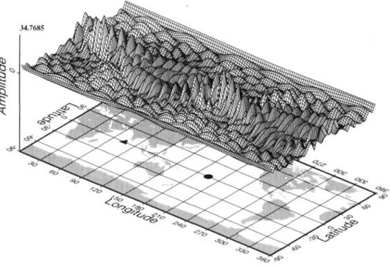
Figs 1-3 show modulation fields at the receiver and source for

the multiplet oS,,. These fields are computed by making the

inverse Legendre transformation of the hybrid modulation

functions at the source and receiver [see Lognonne &

Romanowicz (1990) for details on the discrete Legendre trans- formations]. These fields correspond to the vertical displacement at a depth of 500 km. Due to the small coupling and the

smooth dependence of the spherical eigenfunction on

e,

changes

in depth mainly affect the amplitude of the modulation function and not it shape. The source is a double couple located at a depth of 15 km, along the equator, at 195"E. The mechanism of the source is a vertical strike-slip with a 45" strike. Fig. 1 shows the modulation function of the source at all positions on a 500 km deep sphere. Similarly, Fig. 2 shows the modulation function associated with the receiver. This function shows the amplitude recovered along the vertical axis at all

points of the 500 km deep sphere for an impulsive source. At

t = 0, these modulation functions only differ slightly from the

spherical earth amplitude response. Differences arise only from coupling effects. When time increases, however, and in contrast to the spherical earth case, the modulation function varies, mainly due to the self-coupling; these variations are shown in Figs 3(a)-(d). Figs 3(a) and (b) show the real and imaginary

parts of the source modulation field after 6 hr, while Figs 3(c)

and (d) show these fields after 12 hr. In an aspherical earth, as

noted by Dahlen & Henson (1985) and Henson & Dalhen

(1986), the 2&+ 1 eigenmode singlets have a significant ampli-

0 1996 RAS, G J I 124, 456-482

(6)

FrCchet derivatives of coupled seismograms 461

Modulation function (model

M84)

:

UO

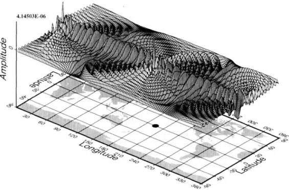
component-real t=Oh multiplet 0,952 - source: double-couple

Figure 1. Modulation field at the source (double-couple) for the multiplet at time t = 0 hr. The vertical component U , is shown at a depth of 500 km. The source is a vertical strike slip with the fault plane oriented at 45" to the equator. Peaks are present at both the location of the source (0.10"N 195"E, 15 km depth, indicated by a black circle on the background map) and its antipode. At the initial time, the field is purely real and is close to the spherical case. This figure could be interpreted as the amplitude of vertical displacement associated with this source for all points on a 500 km depth sphere. For all figures the computation is done using the M84A model of Woodhouse & Dziewonski (1984).

Modulation function (model

M84)

:

UO

component-real - t=Oh multiplet OS52

-

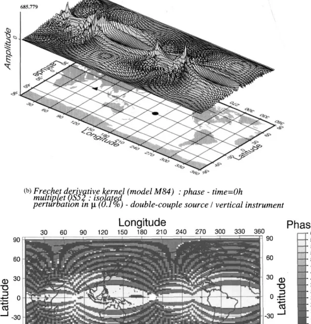
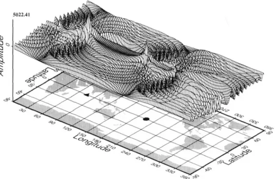
station : vertical component

Figure 2. Modulation field at the station for the multiplet oS,,, at time t = 0 hr. Depth is fixed at 500 km. As for Fig. 1, the U o component of the

field is shown. Peaks are also present at both the receiver location (0.10"N 75"E, indicated by a black triangle on the background map) and its antipode. As in Fig. 1, the field is real and close to the spherical case. This figure gives the displacement recovered at the receiver for a vertical

impulsive source for all points on a 500 km depth sphere. Note that the two peaks have the same sign, due to the even angular order of the mode (this is also true for Fig. 1).

0 1996 RAS, G J l 124, 456-482

(7)

462 E. CltvCdt! and P. Lognonnt!

(4

Perturbation of the modulation function (model M U )

:

UO

component-real t=6h

multiplet

OS52

- source: double-couple

(b)

Perturbation of the modulation function (model M84)

:

UO

component-imaginary t=6h

multiplet

OS52

- source: double-couple

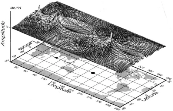
Figure 3. Perturbation of the modulation field at the source for the multiplet $,,, at times t = 6 hr and t = 12 hr. (a) ( t = 6 hr) and (c) ( t = 12 hr)

show the real parts; the field of reference is the modulation at the initial instant (Fig. 1). In the spherical case, this difference is zero. (b) and (d)

show the imaginary part of the modulation fields at times t = 6 hr and t = 12 hr respectively. These fields are equivalent to the absolute ones, since the imaginary part of the modulation field at the initial time is null.

0 1996 RAS, G J I 124,456-482

(8)

FrCchet derivatives of coupled seismograms 463

(c>

Perturbation of the modulation function (model

M84)

:

UO

component-real t=12h

multiplet OS52

-

source: double-couple

(4

Perturbation of the modulation function (model M 8 4 )

: UO

component-imaginary t=12h

multiplet

OS.52 -

source: double-couple

Figure 3. (Continued)

0 1996 RAS, GJI 124,456-482

(9)

464 E. ClCvCdt and P. Lognonnt!

tude along l+ 1 great circles. Each great circle, except one, is

associated with two modes with very close frequencies. Both modulation fields at the source and receiver then select the singlets that possess an antinode at the source or receiver

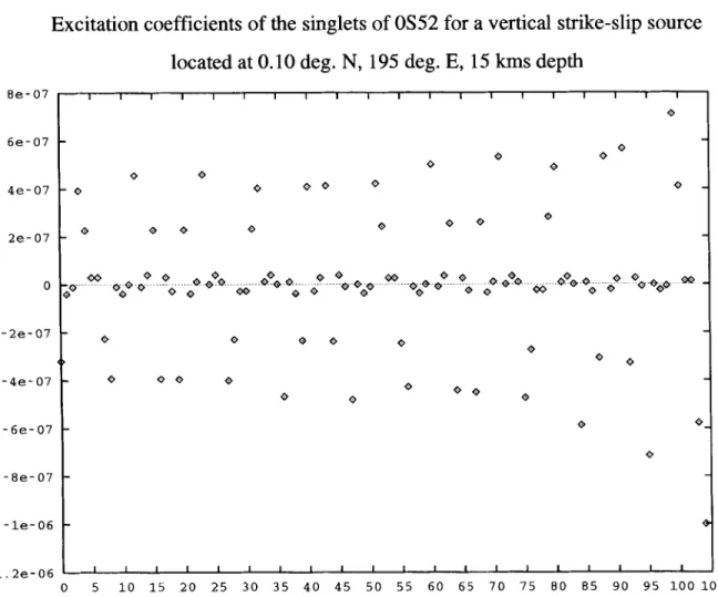
location. As seen in Fig. 4, when the initial amplitudes of the

singlets are plotted, only a few have a significant amplitude. As time increases, the departure from the sphericity of the earth induces slow variations of the initial amplitude. The perturbations with respect to the initial amplitude are concentrated along the singlet great circles with maximum amplitudes.

Note that the perturbation of the modulation function, i.e. its departure from a constant function, is quite significant. The perturbation represents 50 per cent of the initial value after

6 hr, and is equal to the initial field after 12 hr.

We have also computed the modulation field for an isotropic source. It looks, of course, like the modulation field at the receiver (which is also isotropic) when, as in the numerical example shown here, either no lateral variation in attenuation or no rotation is assumed, thus implying the same dual and primal eigenmodes.

5.2 Frechet derivative kernel

The Frkhet derivatives involve modulation functions both at the source and receiver. These FrCchet derivative kernels are

shown in Figs 5-6 for the mode &,. In each of these figures,

the amplitude at a given point with latitude 0 and longitude

I$ is the perturbation in the recorded amplitude modulation

function when a Dirac delta function perturbation is put in

the model M84A at a depth of 500 km and at location 0,

4.

Figs 5(a)-(f) and 6(a)-(f) are for perturbations in the shear modulus. In Figs 5(a)-(f), we show the Frechet derivative obtained only by the self-coupling terms, which are given by

relation (38). Note, however, that coupling is taken into

account in the computation of normal modes, and in the computation of the modulation fields. At the initial time (Figs 5a and b), the kernel appears to have a maximum along the great circle (in our case the equator) connecting the source and the station. The phase plot shows that this 'equatorial peak' is a stationary phase point, giving rise to the asymptotic approximation of the great-circle path average. Our results diverge from the asymptotic approximation, however, by the

8 e - 07 6 e - 0 7 4e- 07 2e-07 0 - 2 e - 0 7 - 4 e - 0 7

-

6 e - 07 - 8e- 07 - le- 06 -1.2e-06

Excitation coefficients of the singlets of OS52 for a vertical strike-slip source

located at

0.10 deg.

N,

195 deg.

E, 15 kms depth

1 1 1 1 1 1 1 1 1 1 1 1 1 1 1 1 1 1 1 1 0 0 Q O 0 Q Q Q Q 0 5 10 15 20 25 3 0 35 40 45 50 5 5 60 6 5 70 75 80 85 90 95 1 0 0 1 0 5 Figure 4. Excitation coefficients of the singlets of the multiplet ,J,,. The source is the vertical strike slip used for Figs 1, 2 and 3. The coefficients

associated with the 26+ 1 singlets (e.g. 105 modes) are plotted in increasing frequency order. Only less than half of the singlets have a significant

amplitude of excitation. The most excited singlets lead to the general pattern of the modulation field, as the great circles corresponding to these singlets are the locations of maximum amplitude.

0 1996 RAS, G J I 124, 456-482

(10)

Frtchet derivatives of coupled seismograms

465

(4

Frechet derivative kernel (model M84)

:

amplitude

-

time=Oh

multiplet OS52

:

isolated

perturbation in

p

(0.1

%)

- double-couple source

1

vertical instrument

(b)

Frechet derivative kernel (model

M 8 4 )

:

phase

-

time=Oh

multip et OS52

:

isolated

pertur

b

ation in p (0.1

%) -

double-couple source I vertical instrument

Figure 5. Isolated multiplet hypothesis: evolution of the Frechet derivatives kernel (double-couple source) for ,S,, for a perturbation in the shear modulus at several instants. The map shows, on all latitudes and longitudes, the perturbation of the recorded demodulated amplitude for the normal mode ,S5*, when a Dirac perturbation of 0.1 per cent of the spherical PREM value is put at the given latitude and longitude, and at a depth of 500 km. The source is the vertical strike slip used for Fig. 1. (a), (c) and (e) show the absolute amplitude of the kernel at times t = 0, 6 and 12 hr respectively. (b), (d) and ( f ) give the corresponding phase. On both the amplitude and phase representation, the source location (same as Fig. I) is indicated by a circle on the background map, and the receiver location (same as Fig. 2) by a triangle. The phase representation is done so that white corresponds to zero, black to 22, and median grey to n. Thus, whiter and darker zones correspond to close phases. Hence, (b) shows that, at the initial instant, the phase takes only values n and 0 (or 2n), so that the kernel is purely real. Moreover, we can see that the equatorial zone is a stationary phase point, as predicted by asymptotic results. In (d) and ( f ) the pattern changes as the kernels become fully complex.

0 1996 RAS, GJI 124, 456-482

(11)

466

E.

Clkvkdk and P. Lognonnk

( c )

Frechet derivative kernel (model

M84)

:

amplitude - time=6h

multiplet

OS.52 :

isolated

perturbation in

p

(0.1

%) -

double-couple source

I

vertical instrument

(4

Frechet derivative kernel (model M 8 4 )

:

phase

-

time=6h

multiplet OS52

:

isolated

perturbation in p

(0.1

%)

- double-couple source

I

vertical instrument

Figure 5 . (Continued)

0 1996 RAS, GJI 124,456-482

(12)

Frichet derivatives of coupled seismograms 467

(el

Frechet derivative kernel (model

M84)

:

amplitude

-

time=12h

multiplet OS52

:

isolated

perturbation in

p

(0.1

%)

- double-couple source

I

vertical instrument

(f)

Frechet derivative kernel (model M84)

:

phase

-

time=12h

multiplet

OS52

:

isolated

perturbation in

p

(0.1

%)

-

double-couple source

I

vertical instrument

0 1996 RAS, G J I 124, 456-482

(13)

468 E. CEtv6dk and P. Lognonni

(a)

Frechet derivative kernel (model

M84)

:

amplitude

-

time=Oh

multiplet

OS52 (coupling along the dispersion branch

:

+-31)

perturbation in

p

(0.1

%)

- double-couple source

I

vertical instrument

(b)

Frechet derivative kernel (model

M84)

:

phase

-

time=Oh

multiplet

OS52

(cou lin along the dispersion branch

:.

+-3j)

perturbation in p

(81

4

-

double-couple source

I

vertical instrument

Figure 6. Coupled multiplets hypothesis: evolution of the Frechet derivatives kernel (double-couple source) for oS,, for a perturbation in the shear

modulus at several instants. The multiplet coupling is done for the six nearest modes around oS5p on the fundamental dispersion branch. Conventions are the same as for Fig. 5. The source mechanism is also the same. Coupling effects clearly appear at short times. These effects are located near strong velocity gradient zones and affect both phase and amplitude. They decrease with time, as the secular terms corresponding to the isolated multiplet contribution increase. (e) ( t = 12 hr) presents the same pattern as Fig. 5(e), the isolated multiplet case. Only the corresponding phase ( f ) still shows differences from the isolated case (Fig. 5f).

0 1996 RAS, G J I 124,456-482

(14)

Fr6chet derivatives of coupled seismograms 469

(c)

Frechet derivative kernel (model M 8 4 )

:

amplitude

-

time=6h

multiplet

OS52

(coupling along the dispersion branch

:

+-31)

perturbation in p

(0.

I

%)

- double-couple source

I

vertical instrument

(4

Frechet derivative kernel (model M84)

:

phase

-

time=6h

multiplet

(IS52

(cou lin along the disp rsion branch

:.

+-31)

perturbation in

p

(81

%$

-

double-coup fe source

I

vertical instrument

0 1996 RAS, G J I 124, 456-482

(15)

410 E . ClCvCd6 and

P.

LognonnC

(el Frechet derivative kernel (model M 8 4 ) : amplitude

-

time=12h multiplet

OS52

(coupling along the dispersion branch : +-31)

perturbation in

p

(0.1 %) - double-couple source I vertical instrument

(0

Frechet derivative kernel (model M 8 4 )

:

phase

-

time=12h

multiplet OS52 (cou lin along the dispersion branch :. +-3.l)

perturbation

in

p

(81

4 -

double-couple source

I

vertlcal instrument

Figure 6. (Continued)

0 1996 RAS, GJI 124, 456-482

(16)

Frkchet derivatives of coupled seismograms 471 fact that the equatorial peak is very broad, and the sides lobes

do not vanish toward the poles. Note that, at t = 0, the kernel

is a purely real quantity, all modulation fields being purely real (there is no aspherical attenuation in our model). As time increases, the maximum of energy moves slowly from its initial location to reach an orbit corresponding to the most excited singlets for the source-receiver couple (Figs 5c and e), while the kernel becomes fully complex. The spherical great-circle approximation is no longer valid; indeed, our FrCchet derivative kernel appears to be essentially sensitive to the structure beneath a path which is not exactly the geometrical great circle, and which slowly precesses with time. We now look at the terms in the Frechet derivative [given by (3911 involving

coupling along a particular dispersion branch. Figs 6(a)-(f )

show the kernels for the same time as in Figs 5(a)-(f). The summation in (39) is only done for the six closest modes along the dispersion branch.

If self-coupling gives sensitivity to even degree structure, coupling along the branch introduces asymmetries (odd struc-

ture) between major and minor arcs and allows us to see

focusing effects (e.g. Romanowicz 1987). Indeed, at t = 0, the

departure from the spherical case is greater than previously. We observe strong focusing effects near strong velocity gradient zones, thus showing that the path-average approximation is

no longer valid. Sensitivity along the R1 path is different from

the sensitivity along the R, path. However, as the self-coupling part is a secular term, with an amplitude that increases fairly

linearly with time, the relative importance of the coupling

terms with respect to the self-coupled terms will vary as

coupled 1

- N

isolated - (oK - o,.)t '

where t is the time. In our example, at time t = 4 hr, the typical

contribution of the coupling effect is more than 50 per cent of the total amplitude. This contribution is the only one that is significantly sensitive to the lateral heterogeneities with odd- order symmetry. Indeed, the self-coupling part, due to the

selection rules, is mostly sensitive to the even part of lateral

heterogeneities even though, in contrast to the case of the FrCchet derivative with respect to a spherical earth, it has a small sensitivity to the odd part (Woodhouse 1983; Romanowicz 1987; Park 1987). As a consequence, the sensi- tivity of the complete FrCchet derivative to lateral variations with odd-order symmetry decreases as time increases. This is especially true for inversions based on resolved normal modes,

which need a long time series (Ritzwoller et al. 1986, 1988;

Giardini et al. 1987, 1988). If we want to use a single reson-

ant peak, it is necessary to separate modes with frequency

differences of ( o K - m K , ) , and the length of the series must

then be such that

(0, - O K ' ) t > 1.

The Frtchet derivative is then dominated by the self-coupling secular term, and therefore mainly sensitive to the even-order lateral variations, confirming numerical results shown by Hara et al. (1993).

We have also computed the Frechet derivative kernels for

the low-angular-order mode oS1,. The computation has been

performed using the same receiver and double-couple source

as for

&,.

Figs 7(a)-(f) shows the Frechet derivative kernel

for a perturbation of 0.1 per cent in p, at the initial time

(Figs 7a and b), after 24 hr (Figs 7c and d ) and after 48 hr

(Figs 7e and f). The same features as previously appear, but here secondary side lobes around the main path are very important, due to the rather low angular order of the

mode oS17. After 48 hr, the main contribution to the amplitude

comes from the secular terms corresponding to the self- coupling part.

Considering Frechet derivative kernels computed for an isotropic source, the comparison with the results obtained with the vertical strike-slip source shows that the amplitude pattern appears to be fairly independent of the mechanism of the source, except near the source location. The difference is in the

phase values,.where in our case a quasi-constant IT dephasing

occurs between the kernels obtained with the two different types of mechanism.

5.3 Local frequency and comparison between elastic/anelastic perturbations

Let us compare our results in the context of local frequency,

and try to address the problem of attenuation sensitivity to

effects of focusing/defocusing (Levshin, Ritzwoller & Ratnikova

1994; Romanowicz 1994). We can define the local frequency associated with a modulation function as

& ( t ) = A,(O) exp[it6a(t)],

so that the perturbation of the local frequency, for short time, is given by

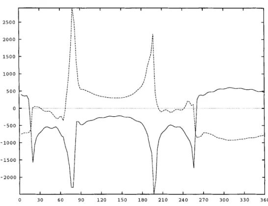
A real perturbation of the local frequency may be, to the first order, and without focusing/defocusing corrections, associated with a real perturbation of the stiffness tensor, while an imaginary perturbation of the local frequency may be associated with the imaginary part. The map of the perturbation of the local frequency of oS52 is shown in Figs 8(a)-(d). The amplitude of the real and imaginary parts along the equatorial

path is shown in Figs 9(a)-( b) and 10(a)-( b), 2 and 4 hr after

the earthquake for perturbations in p and Q p , respectively.

Figs 9(a)-( b) show the predominance of a real perturbation of the local frequency for a real perturbation of the stiffness

tensor over most of the R, and R2 paths, except between the

antipode of the source and the receiver, where focusing is

strong and where both the real and imaginary parts have

terms of equal amplitude.

In contrast, for imaginary perturbations of the stiffness tensor (Fig. 10a-b) we end up with a less pronounced signature on the local frequency: the real perturbation is at least half of the imaginary one, and is even predominant between the antipode of the source and the receiver.

In all cases, we have a strong focusing of the sensitivity near the location of the source, receiver, and their antipodes by a

factor of 3 to 5. Note that the imaginary perturbation of the

local frequency, which appears for a 1 per cent lateral variation

in the shear modulus, is roughly equivalent in amplitude to

the signal associated with a 5 per cent lateral variation in the

imaginary part of the shear modulus.

6 SYNTHETIC FOURIER SPECTRUM

The theoretical results given in Sections 1-4, and illustrated

in Section 5, enable a theoretical seismogram and its partial

0 1996 RAS, GJI 124, 456-482

(17)

412 E . Clkvkdk and P. Lognonnk

(a)

Frechet derivative kernel (model

M 8 4 )

:

amplitude - time=Oh

multiplet

OS17

(coupling along the dispersion branch

+-31)

perturbation in

p

(0.1

%)

- double-couple source

I

vertical instrument

(b)

Frechet derivative kernel (model M84)

:

phase

-

time=Oh

multiplet OSl7 (cou lin along the disp rsion branch

t-31)

perturbation in p (&14

-

double-coup fe source

I

vertical instrument

Figure 7. Coupled-multiplet hypothesis: evolution of the Frechet derivatives kernel for

(0.1 per cent). Conventions are as in Figs 5 and 6. (a) and (b) show, respectively, the amplitude and phase at the initial time. The Frbchet derivative kernels in amplitude and phase are given after 24 hr in (c) and (d), and after 48 hr in (e) and (f).

(double-couple source) for a perturbation in

0 1996 RAS, G J I 124, 456-482

(18)

Fr6chet derivatives of coupled seismograms 413

(c)

Frechet derivative kernel (model

M84)

:

amplitude - time=24h

multiplet OSI 7 (coupling along the dispersion branch +-31)

perturbation in

p

(0.1

96)

- double-couple source

I

vertical instrument

(4

Frechet derivative kernel (model M 8 4 )

:

phase

-

time=24h

rnultiplet

OS17

(cou lin along the disp rsion branch +-3

1 perturbation in p.

(81

-

double-coup fe source

I

vertica

f

instrument

Figure 7. (Continued)

0 1996 RAS, G J I 124,456-482

(19)

474 E . ClPvCdP and P. Lognonnd

( e )

Frechet derivative kernel (model M84)

:

amplitude -

time=48h

multiplet

OS17

(coupling along the dispersion branch +-31)

perturbation in

(0.1

%)

- double-couple source

I

vertical instrument

( f )

Frechet derivative kernel (model M84)

:

phase

-

time=48h

multiplet QSI

7 (cou lin

along the disp rsion branch

t-31)

perturbation in p

($1

%$

-

double-coup

1"

e source

I

vertical instrument

0 1996 RAS, GJI 124, 456-482

(20)

Frdchet

derivatives

of coupled

seismograms

415

(a)

Perturbation

of

the instantaneous frequency (model

M84)

:

real part -

time=2h

multiplet

OS52

(coupling along the dispersion branch

:

+-31)

perturbation in

p

(0.1

%)

- double-couple source

I

vertical instrument

(b)

Perturbation

of

the instantaneous frequency (model M84)

:

imaginary part -

tirne=2h

multiplet OS52 (coupling along the dispersion branch

:

+-31)

perturbation in

p

(0.1

%) -

double-couple source I vertical instrument

Figure 8. Perturbation of the local eigenfrequency of the multiplet ,$,,. These maps show the perturbation of the local frequency, as defined by the relation (42). Conventions are as in Figs 5 to 7. (a) and (b) show the real and imaginary parts of the frequency (depth is 500 km) due to a local variation of the shear modulus of 1 per cent at time t = 2 hr, while (c) and (d) give the field induced by a local variation of the attenuation factor Q , of 10 per cent at the same time. These two kinds of perturbation yield the same order of magnitude for the perturbation of the complex frequency.

0 1996 RAS, GJI 124, 456-482

(21)

416

E . Clevkde and P. Lognonnt

( c ) Perturbation of the instantaneous frequency (model M 8 4 ) : real part

-

time=2h

multiplet OS.52 (coupling along the dispersion branch : +-31)

perturbation in Q, (1

0%)

-

double-couple source I vertical instrument

(dl Perturbation of the instantaneous frequency (model M84) : imaginary part

-

time=2h multiplet OS.52 (coupling along the dispersion branch : +-31)

perturbation in

QF

(10%) - double-couple source I vertical instrument

0 1996 RAS, GJI 124, 456-482

(22)

Frkchet derivatives of coupled seismograms 477 (a) Perturbation of the instantaneous complex frequency of the multiplet OS52 along the equator

perturbation in shear modulus (0.1 %), time=2h, source: double couple, depth=500kms

5 0 0 0 4 5 0 0 4 0 0 0 3 5 0 0 3 0 0 0 2 5 0 0 2 0 0 0 1 5 0 0 1000 5 0 0 0 - 5 0 0 -1000 0 3 0 6 0 9 0 1 2 0 1 5 0 1 8 0 2 1 0 2 4 0 2 7 0 3 0 0 3 3 0 3 6 0

(b) Perturbation of the instantaneous complex frequency of the multiplet OS52 along the equator

perturbation in shear modulus (0.1 %), time=4h, source: double couple, depth=SOOkms

4 0 0 0 3 5 0 0 3 0 0 0 2 5 0 0 2 0 0 0 1 5 0 0 1000 500 0 - 5 0 0 -1000 -1500 -2000 0 30 60 9 0 1 2 0 1 5 0 1 8 0 2 1 0 2 4 0 270 3 0 0 3 3 0 3 6 0

Figure9. Perturbation of the local eigenfrequency of the multiplet oS52 along the equator for a perturbation in p (0.1 per cent). The perturbation is taken along the geometrical great circle, for time t = 2 hr in (a) (extracted from Figs 8a and b), and for time t = 4 hr in (b). The continuous curves represent the real parts of the perturbations, corresponding to apparent phase perturbations, while the dashed lines are for the imaginary parts, producing focusing/defocusing effects or attenuation effects. The real perturbation of the local frequency is predominant for most of the R, and R, paths. In contrast, the loci of strong focusing show an equal contribution to the real and imaginary parts of the local frequency perturbation.

0 1996 RAS, GJI 124, 456-482

(23)

418 E . Cltutd6 and P. Lognonnt

(a) Perturbation of the instantaneous complex frequency of the multiplet OS52 along the equator

2 5 0 0 2 0 0 0 1 5 0 0 1000 5 0 0 0 - 5 0 0 -1000 - 1 5 0 0 - 2 0 0 0 0 3 0 6 0 9 0 1 2 0 1 5 0 1 8 0 2 1 0 2 4 0 270 3 0 0 3 3 0 3 6 0

(b) Perturbation of the instantaneous complex frequency of the multiplet OS52 along the equator

perturbation in Q-shear (lo%), time=4h, source: double-couple, depth=SOOkms

3 0 0 0 2 5 0 0 2 0 0 0 1 5 0 0 1 0 0 0 5 0 0 0 - 5 0 0 -1000 - 1 5 0 0 i 0 3 0 6 0 90 1 2 0 1 5 0 1 8 0 2 1 0 2 4 0 2 7 0 3 0 0 3 3 0 3 6 0

Figure 10. Perturbation of the local eigenfrequency of the multiplet oS52 along the equator for a perturbation in Q, (10 per cent). Conventions are the same as for Fig. 9. (a) is extracted from Figs 8(b) and (c). In this case, the real part of the local frequency perturbation becomes predominant along the shortest paths between the source and receiver locations and their antipodes. Note that a 5 per cent lateral variation in the imaginary part of the shear modulus gives a roughly equivalent amplitude of the local frequency perturbation to that obtained with a 1 per cent lateral variation in the real part of the shear modulus.

0 1996 RAS, G J I 124, 456-482

(24)

Frdchet derivatives of coupled seismograms 479 derivatives to be calculated. In the same way, we can obtain

synthetic spectra through the modulation function formalism.

Nowab & Lognonne (1994) show that for a synthetic

seismogram expressed as

(43)

K

with, following eqs (10) and (12),

A K ( t ) = <RlSK(t)) = <RK(t)lS) 2 (44)

the corresponding Fourier spectrum can be obtained analytically.

If s ( t ) is cut into N segments [T,,, T,,,] of length AT, its Fourier transform can be written as

N

(45) with

f 2 n

s;(o) =

C

A K ( t ) exp [i(uK - w ) t ] S t , (46)

l l n

where 6 t represents the time spacing between data points in

the initial time series, and t,, and tzn are respectively the times

for the first and last points in the nth segment.

As shown by Nawab & Lognonnk (1994), the modulation

function A K ( t ) can be modelled by a cubic polynomial over

each nth segment. This leads to the analytical expression for the Fourier spectrum:

N

4 4

=

1

expCi(0, -

W l ” 1

K n = l

x c ~ K ( T , ) d ; ( w )

+

AK(TI+l)d%4

+

k,(T,)ATd;(w)

+

kK(T,+l)ATd:(w)] 6 t , (47)

where

k,

represents the time derivative of A K , and where the

functions d ; ( o ) , d”,(o), d;(o) and d:(o) depend only on the

spherical frequency of the multiplet and on the number of

points per sequence. Expressions for these functions are

detailed in Nawab & Lognonne (1994). In the same way, the

Frechet derivatives of the spectrum can be calculated using expression (47), by replacing the modulation functions by their Fr6chet derivatives.

7 CONCLUSION

We have formulated expressions for Frechet derivative seismograms for elastic, anelastic and physical dispersion perturbations in a laterally heterogeneous earth model. These results are based on the concept of modulation fields considered independently, either at the sources or at the receivers. These

fields condense all the effects on seismograms produced by

lateral variations of the Earth. They are characterized by slow modulations in time, involving a characteristic time-scale com- parable to the inverse of the frequency splitting width and not to the period of the mode. Moreover, the computation of

N x M seismograms and their related Frechet derivatives only

requires the computation of M source modulation functions

and N receiver modulation functions.

In order to compute the modulation fields rapidly, a ‘direct solution’ technique has been proposed which avoids the computation of the aspherical normal modes. This technique is

based on perturbation theory, expressed up to the second order for amplitudes, and up to the third order for frequencies, using the results of LognonnC (1991). Thus the time-varying modulation functions use the aspherical normal modes implicitly, but need explicitly only the SNRAI spherical harmonic normal modes and coupling matrices. Hence, the FrCchet derivatives of the seismograms can be rapidly computed for every point of an aspherical anelastic 3-D earth.

The numerical tests performed show some large differences from the spherical symmetric case. First, the frozen-path approximation is no longer valid since the sensitivity of the seismogram shifts with time from the initial great-circle path. The path ‘selected’ depends both on the source and receiver characteristics, and on the structure. Secondly, focusing effects

due to the coupling of the closest modes along a single

dispersion branch invalidate the use of a great-circle path average to retrieve the structure. The importance of these coupling effects at small times cannot be neglected, and other-

wise may result in a wrong localization of the lateral

heterogeneities.

Direct inversion of the structural information carried by the modulation functions is already possible (Nawab 1993), as these secondary observables can now be well determined using, for example, the normal-mode demodulation technique pro-

posed by Nawab & Lognonne (1994). The theoretical formu-

lation given here is a first step to global inversion of seismic waveforms. The fast computation of synthetic seismograms through the modulation field approach and the Frechet derivatives of these seismograms with respect to the structural parameters, as well as the fact that the algorithm derived from

this formulation is well adapted to parallel computers, make

this kind of inversion feasible.

A CK NO WL ED G ME NT S

We thank B. Romanowicz and A. Forte for reading this paper

and making helpful comments. We also thank J.-P. Montagner for profitable discussions. This research was supported

by CNRS/INSU under ATP Tomographie and by

CNCPST/IDRIS under contract 500015. This is IPGP contribution 1394.

R E FE R E NC E S

Dalhen, F.A., 1974. Inference of the lateral heterogeneities of the Earth from the eigenfrequency spectrum: a linear inverse problem, Geophys.

J. R. astr. SOC., 38, 143-167.

Dalhen, F.A. & Henson, I.H., 1985. Asymptotic normal modes of laterally heterogeneous Earth, J. geophys. Res., 90, 12 653-12 681. Dziewonski, A.M. & Anderson, D.L., 1981. Preliminary Reference

Earth Model, Phys. Earth planet. Inter., 25, 297-356.

Geller, R.J. & Hara, T., 1993. Two efficient algorithms for iterative linearized inversion of seismic waveform data, Geophys. J. lnt., Giardini, D., Li, X.-D. & Woodhouse, J.H., 1987. Three-dimensional structure of the Earth from splitting in free oscillation spectra,

Nature, 325, 405-41 1.

Giardini, D., Li, X.-D. & Woodhouse, J.H., 1988. Splitting functions of long-period normal modes of the Earth, J. geophys. Rex, 93, 115, 699-710. 13 716-13 742. 0 1996 RAS, G J l 124, 456-482 at INIST-CNRS on October 28, 2016 http://gji.oxfordjournals.org/ Downloaded from