Study of Hyper-Saline Deposits and Analysis of their Signature in Airborne and Spaceborne SAR Data: Example of Death Valley, California
Texte intégral
Figure
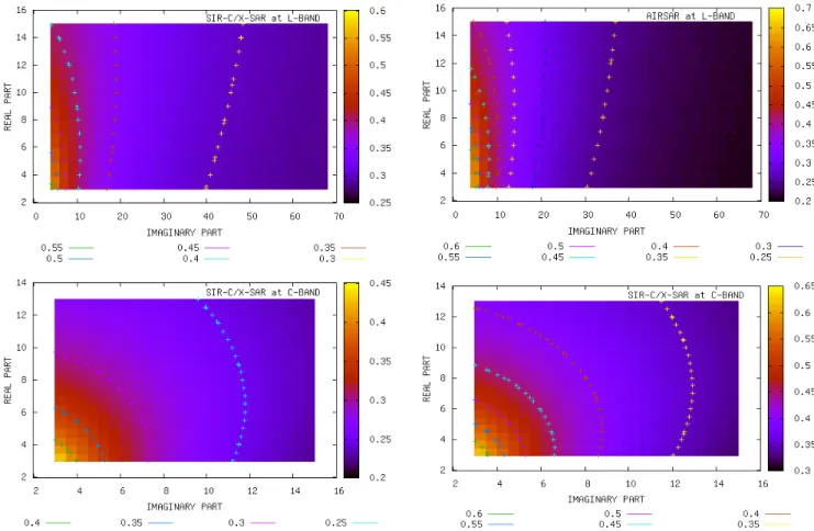
![Fig. 4 displays measurements results of real and imaginary parts of a 100‰-concentrated KCl electrolyte as function of frequency and moisture content in the ranges [500MHz – 7GHz] and [0.05 – 0.6] respectively](https://thumb-eu.123doks.com/thumbv2/123doknet/14792734.602135/10.918.473.847.324.959/displays-measurements-imaginary-concentrated-electrolyte-function-frequency-respectively.webp)

Documents relatifs
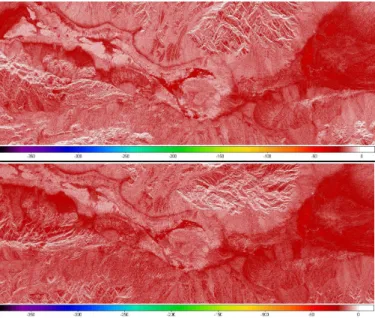
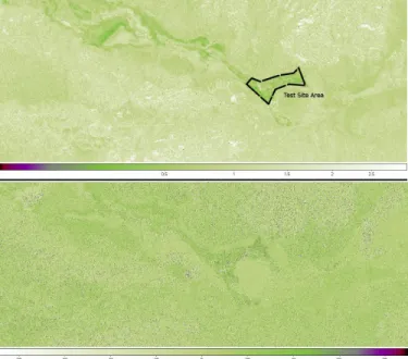
For the grassland plot, until the beginning of April (NDVI < 0.7), the behavior of the SAR signal depends on soil moisture variations: it increases when the soil moisture
In summary, no general purpose algorithm will ever serve all applications or data types (Peel et al. 2016), because each perspective emphasizes a particular core aspect: a cut-
I studied timing of the active season, reproduction, and weight loss during hibernation in Columbian ground squirrels (S. Entry into hibernation and emergence from hibernation
Demonstrating the contribution of dielectric permittivity to the in-phase EMI response of soils: example of an archaeological site in Bahrain... Demonstrating the contribution
Il faut souligner que c’est dans ce canton que se concentre la majorité (33%) des Équatoriennes et Équatoriens résidant (avec ou sans papiers) en Suisse 1. D’un point de vue
[r]
L’archive ouverte pluridisciplinaire HAL, est destinée au dépôt et à la diffusion de documents scientifiques de niveau recherche, publiés ou non, émanant des
Our aim was to assess the prevalence and the determining factors of epileptic seizures anticipatory anxiety in patients with drug-resistant focal epilepsy, and the
