HAL Id: insu-01295492
https://hal-insu.archives-ouvertes.fr/insu-01295492
Submitted on 31 Mar 2016
HAL is a multi-disciplinary open access
archive for the deposit and dissemination of
sci-entific research documents, whether they are
pub-lished or not. The documents may come from
teaching and research institutions in France or
abroad, or from public or private research centers.
L’archive ouverte pluridisciplinaire HAL, est
destinée au dépôt et à la diffusion de documents
scientifiques de niveau recherche, publiés ou non,
émanant des établissements d’enseignement et de
recherche français ou étrangers, des laboratoires
publics ou privés.
Long-term persistence of the spatial organization of
temperature fluctuation lifetime in turbulent air
avalanches
C Crouzeix, J.-L Le Mouël, F Perrier, M. Shnirman, E Blanter
To cite this version:
C Crouzeix, J.-L Le Mouël, F Perrier, M. Shnirman, E Blanter. Long-term persistence of the spatial
organization of temperature fluctuation lifetime in turbulent air avalanches. Physical Review E :
Statistical, Nonlinear, and Soft Matter Physics, American Physical Society, 2006, 74 (3), pp.036308.
�10.1103/PhysRevE.74.036308�. �insu-01295492�
Long-term persistence of the spatial organization of temperature fluctuation lifetime
in turbulent air avalanches
C. Crouzeix,1J.-L. Le Mouël,1F. Perrier,1M. G. Shnirman,1,2and E. Blanter1,2
1Équipe de géomagnétisme, Institut de physique du Globe, Boîte Postale 89, 4 place Jussieu, 75252 Paris cedex 05, France 2International Institute for Earthquake Prediction Theory and Mathematical Geophysics, Warshavskoe shosse, 79, korp2,
Moscow 113556, Russia
共Received 19 September 2005; published 27 September 2006兲
It has been recently proposed that some natural phenomena, such as sunspot occurrence, can be represented by a modulated Markov jitter, which is a high-frequency Markov signal multiplied by a long-term component. The two parameters of this model can be estimated using a nonlinear method based on absolute derivatives. This analysis is applied here to a different physical system: the temperature time series measured during air avalanches in the vertical access pit of an underground quarry. The thermal fluctuations associated with these turbulent flows, driven by the external temperature forcing, actually appear as another practical realization of a modulated Markov jitter. One parameter of the model provides the lifetime of the temperature fluctuations, which can be estimated as a function of time and position. The obtained lifetime is of the order of 10 to 25 min, and is remarkably constant in time for each sensor, independently of the amplitude of the forcing. Furthermore, a significant and persistent spatial structure is observed, revealing a long-term intrinsic organization of the turbulent air flows in the pit. Such a stable spatial organization may reflect a general feature of turbulent phenomena.
DOI:10.1103/PhysRevE.74.036308 PACS number共s兲:
47.27.E-I. INTRODUCTION
Nonequilibrium turbulent systems are a fascinating area of research and, in particular, they exhibit an amazing ability to organize themselves into persistent structures关1兴. The ori-gin of this spatial organization and its emergence in noisy or chaotic environments are poorly understood at the moment. This organization is mainly investigated in well-controlled Rayleigh-Bénard experiments where, in the hard-turbulence regime, the onset of large-scale circulation appears con-nected to the statistical properties of plumes 关2,3兴. Such phenomena are not specific to particular laboratory experi-ments, however, but seem to be universal, pervading natural processes at all scales关4兴.
It is interesting to develop simple representations with few parameters whose spatial and temporal variations can be studied easily. One representation has demonstrated a defi-nite relevance in the case of sunspots关5兴: a high-frequency Markov process 关6兴 multiplied by a long-term component, the modulated Markov jitter. Using a simple nonlinear tech-nique based on the absolute derivative, one parameter of the signal, its lifetime, has been determined and, in the case of sunspots, observed to increase with time关7兴. This leads us to search for other realizations of the modulated Markov jitter in different natural contexts.
In a previous paper 关8兴, we analyzed the properties of turbulent air avalanches in the 20-m-deep vertical access pit to an underground cavity. The aim of this paper was to de-scribe the properties of turbulent flows in a medium-scale natural system and discuss it in the light of Rayleigh-Bénard 共RB兲 convection and general turbulence, e.g., 关9兴. Obviously, this system differs from the standard RB experiments, in particular because of its boundary conditions: at the top and at the bottom of the pit, exchanges take place with the out-side and with the quarry; heat transfers also occur at the
walls. This system is thus open and nonadiabatic.
Air avalanches take place in the pit when the outside air density is larger than the equilibrium air density in the quarry, thus most of the time in winter, when the outside air is colder than the quarry air. During this regime, the mean Rayleigh number Ra is estimated to be about 1012, and the Prandtl number Pr of air is about 0.7. Temperature measure-ments performed along a vertical profile show that the ava-lanches are associated with a mean vertical temperature pro-file and with broadband, spatially organized, and coherent temperature fluctuations 关8兴. This analysis has shown that persistent structures of the flow can be observed, apparently imposed by the boundary conditions.
In the present paper, we are not investigating further the underlying fluid dynamics of the air avalanches in the frame-work of standard RB convection. Rather, we study the rel-evance of a modulated Markov jitter to describe the tempera-ture time series observed in the pit. As developed in the case of sunspots, we apply our method of absolute derivatives and we study the spatial and temporal variations of the estimated parameters, independently of any a priori assumption on the nature of the turbulent flows.
We first recall the properties of the modulated Markov jitter, and we briefly describe the site and the experimental setup and state the results obtained in previous studies. The method of absolute derivatives is then applied to the tem-perature time series and we study the estimated lifetime as a function of time and position. The relevance of the modu-lated Markov jitter is discussed in the conclusion in relation with sunspots.
II. MODULATED MARKOV JITTER
Modulated Markov jitter was proposed to represent the sunspot activity by Blanter et al.关5兴. We succinctly recall its
properties here. The signal ⌰共t兲, taken as a positive real number, is written as
⌰共t兲 =共t兲F共t兲, 共1兲
i.e., the product of a long-term共low-frequency兲 component F and a high-frequency component, referred to as the jitter. The conditions of validity of the representation共1兲 are dis-cussed by Blanter et al.关5兴. Grossly speaking, it is valid if the⌰共ti兲 time series is similar to the time series made of its discrete absolute derivative, defined as
兩⌰
⬘
共ti兲兩 =兩⌰共ti+1兲 − ⌰共ti兲兩
␦t , 共2兲
where ␦t = ti+1− ti is the sampling interval. In practice, the choice of such a simple model is justified by the results. Let us point out that absolute values of turbulence parameters 共velocity and temperature increment兲 have already been used, although in a different way 关10,11兴. Taking absolute values enhances the effect of positive and negative fluctua-tions, while they are canceled when simple moving averages are computed.
Here, we further assume that the jitter has the following form:
共ti+1兲 =␣共ti兲 +共ti+1兲. 共3兲 Equation共3兲 is the general form of an autoregressive Markov process of first order; the first term of the right-hand side is what remains at time ti+1of the value of the process at time ti, whereas the second termis a newly generated flow. The autoregression coefficient␣characterizes the correlation be-tween the two successive variables 共ti+1兲 and 共ti兲. In Blanter et al.关5兴, the random variableis arbitrarily taken as uniformly distributed on the interval共0,1兲, 苸 艛关0,1兴. In the present paper, we rather consider a binomial variable = B共p兲; = 1 with probability p, and = 0 with probability 共1−p兲.
We assume, for the sake of simplicity, the low-frequency modulation F positive and sinusoidal with a period T. Here, this represents the daily modulation of the pit temperature due to the daily external forcing. In order to investigate the properties of the high-frequency component , we have to eliminate the influence of the modulation F. Therefore, most of the time, we will average ⌰共ti兲 over time intervals of length T using ⌰T共ti兲 = 1 Nk=i−n
兺
i+n ⌰共tk兲, 共4兲with T = N␦t and N = 2n + 1. The mean lifetime can be written关5兴
= ␦t
1 −␣. 共5兲
To estimatefrom⌰共ti兲, we introduce the inverse relative variation共IRV兲 of the signal as the ratio of the mean value of the signal to the mean value of its absolute derivative:
rT共t兲 = ⌰T共t兲 兩⌰
⬘
兩T共t兲. 共6兲
The average value over T of the modulated Markov jitter defined by Eqs.共1兲 and 共3兲, with 苸B共p兲, is approximately
⌰T共t兲 =
pFT共t兲
1 −␣ , 共7兲
and the average of its absolute derivative is 兩⌰
⬘
兩T共t兲 =2p共1 − p兲FT共t兲
␦t . 共8兲
The IRV thus does not depend on the modulation F, but only reflects the properties of the high-frequency component:
rT共⌰兲 = r = ␦ t
2共1 − p兲共1 −␣兲. 共9兲 The Parameter p is also estimated from the data; a practical estimator is the relative frequency of positive values of ⌰
⬘
共t兲:pˆ = P兵⌰共ti+1兲 − ⌰共ti兲 ⬎ 0其. 共10兲
The estimate of the lifetimeˆrthrough r is given by
ˆr= 2共1 − pˆ兲r. 共11兲
III. THE SITE AND THE EXPERIMENTAL SET-UP
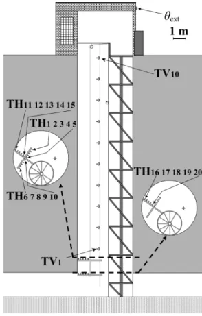
The abandoned “La Brasserie” limestone quarry is located 18 m below ground surface under the park of Vincennes near Paris 关12兴. It consists of pillars and rooms with a height varying from 2 to 7 m, and a total air volume of approxi-mately 60 000 m3. The quarry is connected to the ground surface by a single large access pit 共Fig. 1兲 with 4.56 m diameter. This pit of height h = 20 m can thus be considered as a vertical pipe linking the outside atmosphere, where tem-perature and relative humidity 共RH兲 vary on daily and sea-sonal cycles, to a finite but large volume of air at 12.7 ° C and 100% RH. A metallic staircase of diameter about 2.2 m slightly obstructs the air flow, leaving a free area of 15.4 m2 in the pit. The upper part of the pit reaches into a building, but broken panes in windows with a surface area of about 2.3 m2 allow air exchange with the outside atmosphere.
Half of the year, as long as the outside air density is larger than the equilibrium density of the quarry air, avalanches take place in the pit关13兴, producing natural ventilation of the whole quarry. The presence of this natural ventilation is con-firmed by the seasonal variation of the radon concentration 关14兴, which indicates ventilation rates varying from 0.03 to 0.14 m3s−1. The air temperature in the quarry has an average value of0= 12.7 ° C with yearly variations of the order of 0.16 ° C. The relative humidity is larger than 99.8% in non-ventilated conditions, and varies from 99.2% to 99.8% dur-ing ventilated conditions in winter.
Temperature measurements in the pit are performed with two setups关8兴. The first one is a vertical profile located about 65 cm away from the staircase, and consisting in ten points
CROUZEIX et al. PHYSICAL REVIEW E 74, 036308共2006兲
separated by 1.75 m, labeled TV1–TV10共Fig.1兲. Because of their finite size, the thermistors have a response time of the order of 30 s. The second setup consists in four horizontal branches of five thermistors each, with a regular spacing of 18 cm. Three branches are located at the same level, and the fourth branch 1.3 m below, as indicated in Fig.1. The sam-pling time interval is 2 min. The outside temperature is re-corded above the entrance door of the quarry pit building, with 1 h sampling interval.
IV. WINTER TEMPERATURE RECORDINGS; PREVIOUS RESULTS
Temperatures recorded outside and along the vertical profile during four days of December 2003 are shown in Fig. 2共a兲. Note that the temperature in the upper part of the pit 共TV9兲 is almost the average between the outside temperature
ext and the equilibrium temperature of the quarry 0; this fact indicates a vigorous mixing of the air in the pit during the avalanches. Figure2共b兲presents the temperature aver-aged using Eq.共4兲 with T equal to one day. A linear vertical profile of temperature is observed, which reflects heat ex-changes at the wall关8,13兴. The slope of this profile depends on the forcing.
During the winter regime, short-period fluctuations of the order of 1 ° C peak to peak, which reflect the air avalanches, are noticed on all the sensors of the vertical profile.
Distri-butions of these temperature fluctuations are nearly Gaussian and their power density spectra are almost constant in the range from 3⫻10−4 to 4⫻10−3Hz, also a consequence of the heat transfers occurring at the wall 关8兴. These tempera-ture fluctuations, which are coherent from sensor to sensor, have a standard deviation proportional to the temperature difference between the upper part of the pit and the equilib-rium temperature of the quarry关13兴. This property leads us to propose that the temperature fluctuations, from a statistical point of view, can be represented by a modulated Markov jitter.
V. APPLICATION TO THE PIT TEMPERATURE TIME SERIES
In the following, we define the signal as
⌰共t兲 =0−共t兲 共12兲 with0= 12.7 ° C the mean temperature in the quarry during December 2003. This temperature 0 can be determined from the data themselves. Indeed, in Fig.3,兩⌰
⬘
兩Tis shown as a function of ⌰T for the various sensors of the vertical setup.兩⌰⬘
兩Tvaries linearly with⌰T. All lines cross兩⌰⬘
兩T= 0 almost at the same point; this value is determined to be0⯝12.7 °C.
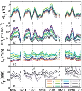
We consider first the data of December 2003 and January 2004 during which the outside temperature remained lower than the equilibrium temperature of the quarry, maintaining a winter regime. We compute⌰T共t兲 and 兩⌰
⬘
兩T共t兲 using Eqs. 共4兲 and共2兲, with T equal to one day.Figure4共a兲displays the curves⌰T共t兲 for sensors 1 to 9 of the vertical setup共see Fig.1兲. It is quite remarkable how the nine curves are proportional to each other, even in their tiny features. Figure4共b兲 displays the nine corresponding curves
FIG. 1. Sketch of the access pit showing the vertical and the horizontal setups, TV and TH, respectively, and the location of the sensor measuring the outside temperatureext.
6 8 10 12 θ ( °C) (a) 0 5 10 θext ( °C) 6 8 10 12 θT ( °C) (b) 0 5 10 θext T ( °C) 0.05 0.1 0.15 0.2 0.25 1 6 2 7 3 8 4 9 5 ext |Θ ʼ|T ( °C min −1 ) (c) 12/160 12/17 12/18 12/19 12/20 5 10 15 20 25 rT (min) (d)
FIG. 2.共Color兲 Data recorded by the vertical set-up during four days of December 2003;共a兲 shows the raw data, i.e. temperature measured outside 共ext兲, and by sensors 1 to 9 of the set-up; 共b兲 corresponds to the moving average calculated with Eq.共4兲 and T
equal to one day;共c兲 is the absolute derivative 兩⌰⬘兩Tas described by Eqs.共2兲 and 共4兲; and 共d兲 is the ratio rT共Eq. 共6兲兲.
兩⌰
⬘
兩T共t兲. Again the 兩⌰⬘
兩T curves are strikingly similar, al-though a little less similar than are the⌰T curves. Further-more, the ⌰T curves are similar to the 兩⌰⬘
兩T curves, as al-ready indicated by Fig. 3. This is the first condition for considering a modulated Markov jitter, as described by Blanter et al.关5兴. The amplitude of the long-term variations of ⌰T共z,t兲 decreases when z, counted greater than 0 down-ward, increases, whereas the amplitude of the corresponding variations of兩⌰⬘
兩T共z,t兲 is remarkably constant when z varies, although to a lesser degree for the two uppermost sensors 共see also 关8兴 and 关13兴兲.Figures 5共a兲 and 5共b兲 display the curves ⌰T共t兲 and 兩⌰
⬘
兩T共t兲, respectively, calculated with the data of thehorizontal setup during the same period as for Fig. 4. By contrast with the vertical setup,⌰T共t兲 is now almost constant horizontally, while 兩⌰
⬘
兩T共t兲 varies from one sensor to an-other. However, ⌰T共t兲 and 兩⌰⬘
兩T共t兲 keep their similarity in time.According to Eq.共6兲, we compute the ratio rT共tk, xi兲 for each sensor of the two setups, at each time tkand each posi-tion xi关Figs. 4共c兲,5共c兲, and5共d兲兴. The ratio rT共tk兲 is fairly constant with time at each depth for the seven lower sensors 关Fig. 4共c兲兴, and for most of the sensors of the horizontal profile关Fig. 5共c兲兴. Larger irregularities, with time constants of a few days, are present on the curves relative to sensors 8 and 9 of the vertical setup, and to sensors 5, 11, and 16–20 of the horizontal setup.
Finally, to get a global description of the spatial variations of the properties of the signal, we compute the average value ⌰T and 兩⌰
⬘
兩T of ⌰共tk, zi兲 and 兩⌰⬘
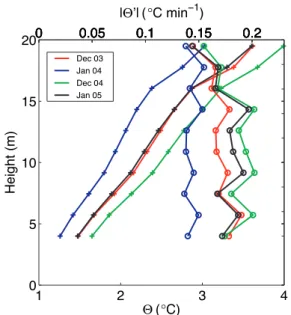
兩共tk, zi兲 from the vertical profile over four periods of ten days each, in December 2003, January 2004, December 2004, and January 2005. The distributions with depth of⌰Tand兩⌰⬘
兩Tare reported in Fig.6. The vertical profiles of⌰Tare almost linear with depth, as previously observed关8兴. The slope with z varies with time, and increases with the forcing, i.e., when the outside tem-perature decreases. Vertical variations of 兩⌰
⬘
兩T are weak. Like ⌰T, 兩⌰⬘
兩T increases with the forcing, but its variation with z remains identical.Figure7represents the vertical profiles of the correspond-ing time averaged ratio r, computed over the same periods. As expected, in a first approximation, the shape of the profile is linear with depth. Its variations with time are small, and unrelated to the forcing.
The time-averaged ratio r, computed during December 2003 and January 2004 over two periods of ten days each, is shown in Fig.8 versus the distance between the sensor and
7 8 9 10 11 12 13 0 0.05 0.1 0.15 0.2 0.25 0.3 |Θ ʼ| T ( °C min −1 ) θT (°C)
FIG. 3. 共Color兲 Absolute derivative 兩⌰⬘兩Tas a function of mean temperatureTfor sensors 1–9 of the vertical setup during
Decem-ber 2003. The linear trend共black line兲 calculated for each sensor is represented to estimate0= 12.7 ° C. The color code is the same as for Fig.2. 0 2 4 6 Θ T ( °C) (a) 0 0.1 0.2 0.3 |Θ ʼ| T ( °C mi n −1 ) (b) 12/07 12/14 12/21 12/28 01/04 01/11 01/18 01/25 0 5 10 15 20 25 r T (min) (c)
FIG. 4. 共Color兲 Data recorded by the vertical setup during De-cember 2003 and January 2004;共a兲 shows the moving average ⌰T
calculated with Eq.共4兲 and T equal to one day; 共b兲 is the absolute
derivative兩⌰⬘兩Tas described by Eq.共2兲; and 共c兲 is the ratio rT关Eq.
共6兲兴. The color code is the same as for Fig.2.
0 1 2 3 Θ T ( °C) (a) 0 0.1 0.2 0.3 |Θ ʼ|T ( °C mi n −1 ) (b) 0 10 20 r T (min) (c) 12/07 12/14 12/21 12/28 01/04 01/11 01/18 01/25 0 10 20 r T (min) (d) 1 6 2 7 3 8 4 9 5 10 11 16 12 17 13 18 14 19 15 20
FIG. 5. 共Color兲 Data recorded by the horizontal setup during December 2003 and January 2004;共a兲 shows the moving average ⌰Tcalculated with Eq.共4兲 and T equal to one day; 共b兲 is the
abso-lute derivative兩⌰⬘兩Tas described by Eqs.共2兲 and 共4兲; and 共c兲 and
共d兲 represent the ratio rT 关Eq. 共6兲兴 for sensors 1–15 and 16–20,
respectively.
CROUZEIX et al. PHYSICAL REVIEW E 74, 036308共2006兲
the wall of the pit. For sensors 1 to 15 共plain lines兲, r de-creases with horizontal distance. For sensors 16 to 20共dotted lines兲, which are placed lower 共see Fig.1兲 and are actually located more in the quarry air than in the pit, r increases with distance to the wall.
To summarize, in the case of the vertical temperature pro-file, the amplitude of ⌰T varies with position, while 兩⌰
⬘
兩T remains constant. In the case of the horizontal profile, it is the opposite: 兩⌰⬘
兩T varies with position, while ⌰T remains constant. The vertical spatial variation of the IRV is thus due to ⌰T whereas its horizontal variations is due to 兩⌰⬘
兩T. In both cases, the obtained IRV is stable with time.VI. DETERMINATION OF LIFETIME AND DISCUSSION
Having observed that the model of modulated Markov jitter can be used to describe the cold avalanches in the quarry pit, we can now determine the values of the two parameters of this model: p and. The value of pˆ, ob-tained from Eq. 共10兲, is 0.50±0.01, stable with time. No dependence versus position is observed.
The lifetimeis the most interesting parameter because it bears a direct physical interpretation. It represents the mean duration of the cold avalanches at a given point. For a sam-pling time of 2 min, using Eq.共11兲, we obtain values varying from 8 min for sensor 1 to 14 min for sensor 7共Fig.7兲. For the horizontal profiles, considering sensors 1–15共full lines in Fig. 8兲, the obtained value is about 15 min near the wall, decreasing to 8 min at 0.8–1.2 m from the wall. These val-ues are significantly larger than the response time of the sen-sors共10–30 s, see Sec. III兲. When data with a shorter sam-pling time are used, for example 10 s, the inferred values using Eq.共11兲 are three times smaller; however, pˆ does not change.
The fact that the lifetime does not depend on time and thus on the forcing, which, equivalently, means that the ava-lanches are adequately represented by a simple modulated Markov jitter, is nontrivial. Also, the fact that the spatial structure of the lifetime persists with time provides a signifi-cant additional information. The flow, organized in a stable manner, has an intrinsic dynamics, independent of the forc-ing. Despite the inherently turbulent nature of the air ava-lanches, a spatial coherence is remarkably maintained in the system, maybe by the heat exchange at the wall. Thus, con-trary to expectations, the cold avalanches do not mix and wash away spatial structures in the pit, but create and main-tain their own. Cermain-tainly a robust and efficient mechanism is needed, but its mode of operation remains unclear. Such mechanisms seem to emerge in various types of natural systems at all scales关1,4兴.
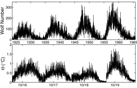
The modulated Markov jitter was noted to be also a good representation of the sunspot Wolf number as a function of
1 2 3 4 0 5 10 15 20 Dec 03 Jan 04 Dec 04 Jan 05 Θ (°C) Height (m) 0 0.05 0.1 0.15 0.2 0 0.05 0.1 0.15 0.2 0 0.05 0.1 0.15 0.2 0 0.05 0.1 0.15 0.2 |Θʼ| (°C min−1)
FIG. 6.共Color兲 Mean vertical profiles of ⌰共+兲 and 兩⌰⬘兩 共ⴰ兲, each computed over ten days during December 2003, January 2004, De-cember 2004, and January 2005.
10 15 20 25 0 5 10 15 20
r (min)
Height (m
)
FIG. 7.共Color兲 Mean vertical profiles of r, each computed over ten days during December 2003, January 2004, December 2004, and January 2005. The color code is the same as for Fig.6.
0 0.2 0.4 0.6 0.8 1 1.2 8 10 12 14 16 18 20 22 24 r (min) Distance (m)
FIG. 8. Mean horizontal profiles of r as a function of the dis-tance from the wall, each computed over ten days during December 2003共+兲, and January 2004 共ⴰ兲. Bold lines correspond to sensors 1–10, normal lines to sensors 11–15, and dotted lines to sensors 16–20.
time 关5,7兴. Recall that the Wolf number is defined as s + 10g where s and g are the spot and spot group numbers, respectively. In the case of sunspots, the modulation has the dominating 11 yr period of the intensity of the solar mag-netic field, while in the case of the air avalanches, it is a diurnal modulation. The similarity between the temperature time series in the quarry pit and the sunspot Wolf number is actually striking in Fig.9. In both cases, modulated Markov jitter offers a simple and adequate representation. The Sun and the access pit are undoubtedly two different physical systems; however, an analogy between the air avalanches and the sunspots may be worth contemplating. An interpre-tation of sunspots generated by plumes dragging the toroidal
magnetic field up to the Sun’s surface might justify this anal-ogy 关15–17兴. The analysis presented in this paper could be applied to other time series and reveal that other natural phenomena can be modeled by a modulated Markov jitter.
ACKNOWLEDGMENTS
The authors thank the Inspection Générale des Carrières and the City of Paris for the access to the Vincennes quarry. Patrick Richon and Pierre Morat are also thanked for their contributions to the experiments. This is IPGP contribution number 2164.
关1兴 L. P. Kadanoff, Phys. Today 54共8兲, 34 共2001兲.
关2兴 K. R. Sreenivasan, A. Bershadskii, and J. J. Niemela, Phys. Rev. E 65, 056306共2002兲.
关3兴 H.-D. Xi, S. Lam, and K.-Q. Xia, J. Fluid Mech. 503, 47 共2004兲.
关4兴 B. I. Shraiman and E. D. Siggia, Nature 共London兲 405, 639 共2000兲.
关5兴 E. M. Blanter, M. G. Shnirman, and J.-L. Le Mouël, J. Atmos. Sol.-Terr. Phys. 67, 521共2005兲.
关6兴 M. Iosifescu, Finite Markov Processes and Their Applications 共John Wiley and Sons, Chichester, 1980兲.
关7兴 E. M. Blanter, J.-L. Le Mouël, F. Perrier, and M. G. Shnirman, Sol. Phys.共to be published兲.
关8兴 F. Perrier, J.-L. Le Mouël, V. Kossobokov, C. Crouzeix, P. Morat, and P. Richon, Eur. Phys. J. B 46, 563共2005兲.
关9兴 X.-L. Qiu and P. Tong, Phys. Rev. E 66, 026308:1 共2002兲. 关10兴 S. I. Vainshtein and K. R. Sreenivasan, Phys. Rev. Lett. 73,
3085共1994兲.
关11兴 S.-Q. Zhou and K.-Q. Xia, Phys. Rev. Lett. 89, 184502:1 共2002兲.
关12兴 C. Crouzeix, Ph.D. thesis, Institut de Physique du Globe de Paris, 2005共unpublished兲.
关13兴 F. Perrier, P. Morat, and J.-L. Le Mouël, Phys. Rev. Lett. 89, 134501:1共2002兲.
关14兴 F. Perrier, P. Richon, C. Crouzeix, P. Morat, and J.-L. Le Mouël, J. Environ. Radioact. 71, 17共2004兲.
关15兴 S. K. Solanki, Astron. Geophys. 43, 5.09 共2002兲.
关16兴 S. K. Solanki, M. Schüssler, and M. Fligge, Nature 共London兲
408, 445共2000兲.
关17兴 E. Friis-Christensen and K. Lassen, Science 254, 698 共1991兲. 1925 1930 1935 1940 1945 1950 1955 1960 1965 0 100 200 300 Wolf Number 10/16 10/17 10/18 10/19 0 0.5 1 1.5 2 Θ ( °C)
FIG. 9. Time series of Wolf number from 1924 to 1966 with a sampling time of one day, compared with a time series of⌰ with a sampling time of 2 min measured during four days of October 2004.
CROUZEIX et al. PHYSICAL REVIEW E 74, 036308共2006兲