Springtime transition in lower thermospheric atomic oxygen

HAL Id: insu-01627448

https://hal-insu.archives-ouvertes.fr/insu-01627448

Submitted on 22 Dec 2020

HAL is a multi-disciplinary open access

archive for the deposit and dissemination of

sci-entific research documents, whether they are

pub-lished or not. The documents may come from

teaching and research institutions in France or

abroad, or from public or private research centers.

L’archive ouverte pluridisciplinaire HAL, est

destinée au dépôt et à la diffusion de documents

scientifiques de niveau recherche, publiés ou non,

émanant des établissements d’enseignement et de

recherche français ou étrangers, des laboratoires

publics ou privés.

Springtime transition in lower thermospheric atomic

oxygen

Gordon G. Shepherd, Jacek Stegman, Patrick Espy J., Charles Mclandress,

Gérard Thuillier, R. H. Wiens

To cite this version:

Gordon G. Shepherd, Jacek Stegman, Patrick Espy J., Charles Mclandress, Gérard Thuillier, et al..

Springtime transition in lower thermospheric atomic oxygen. Journal of Geophysical Research Space

Physics, American Geophysical Union/Wiley, 1999, 104 (A1), pp.213-223. �10.1029/98JA02831�.

�insu-01627448�

JOURNAL OF GEOPHYSICAL RESEARCH, VOL. 104, NO. A1, PAGES 213-223, JANUARY 1, 1999

Springtime transition in lower thermospheric atomic oxygen

G. G. Shepherd,

1 J. Stegman,

2 P. Espy,

TM

C. McLandress,

1 G. Thuillier,

5 and

R.H. Wiens

1

Abstract. Observations

from three optical ground stations

and the wind imaging interferometer

on

the upper atmosphere

research

satellite

have been combined

to describe

a "springtime

transition"

in

atomic oxygen. At each station

the transition

is characterized

by a rapid 2-day rise in the night-time

oxygen

airglow emission

rate by a factor of between

2 and 3, with a subsequent

decrease

by a factor

of about 10 in the same period of time. This latter state of extremely weak oxygen airglow indicates

a depletion

of atomic oxygen that persists

for many days. The characteristic

signature

is similar at

both mid-latitude and high-latitude

stations

and is also observed

in the hydroxyl airglow, except

that immediately following the enhancement,

the hydroxyl emission

rate does not fall below the

value it had before the event. Airglow rotational temperatures

behave coherently

with the emission

rate. WINDII data show that the airglow emission

rate perturbation

is a planetary

scale feature

associated

with strong vertical motions and that the event may be associated

with the winter-to-

summer

zonal wind reversal.

Data from the northern

springtimes

of 1992 and 1993 are reported

upon in detail, with additional

data from 1995 to confirm the persistence

of the phenomenon.

1. Introduction

The wind imaging interferometer (WINDII) on the upper atmosphere research satellite (UARS) measures upper atmospheric winds and emission rates from airglow-excited species [Shepherd et al., 1993]. During the validation of WINDII [Gault et al., 1996; Thuillier et al., 1996], ground-based

instruments were operated at Bear Lake, Utah (42øN, 212øE), and

the Observatoire de Haute-Provence (41øN, 6øE) in southern France. In early April, 1992, the night-time observations at Bear

Lake showed an increase in the emission rate of the 0 2

atmospheric (0,1) band, by a factor of about 2 in just 2 days, followed immediately by a dramatic drop of more than a factor of

10 in the days following. The emission rate remained low for about 5 days, before making a partial recovery and then returning to lower values again. This behavior closely resembled an effect

previously discovered at Stockholm (60øN, 20øE) [Stegrnan et al.,

1992]. Although the Stockholm winter is normally marked by enhancements in airglow emission rate, followed by rapid decreases to the original level, the end of winter is marked by a similar enhancement with one distinct difference. During the

winter the emission rate before and after the enhancement is the

same, but for the springtime event the emission rate following the

enhancement is much lower than that before and lower than that

observed at any time during the winter. The behavior at Stockholm is slightly different from that at Bear Lake in that the emission rate may remain low for several weeks, not returning to

•Centre for Research in Earth and Space Science, York University,

Toronto, Ontario, Canada.

2Arrenius Laboratory, Stockholm University, Stockholm. 3Space Dynamics Laboratory, Utah State University, Logan.

4Department of Physical Sciences, Embry-Riddle Aeronautical University, Daytona Beach, Florida.

•Service d'A6ronomie, Verri•res-le-Buisson, France.

Copyright 1999 by the American Geophysical Union. Paper number 98JA02831.

0148-0227/99/98J A-02831 $09.00

normal values again before the onset of summer high-latitude daylight. The winter events are associated with stratospheric warmings, while the focus in this paper is directed solely toward this springtime feature. Here we show data for four springtime periods, but J. Stegman (manuscript in preparation, 1998) presents in detail the behavior from 1985 to 1997, clearly showing that the basic characteristics do repeat year after year. A

similar effect was found for the Observatoire de Haute-Provence.

Since the nighttime oxygen airglow is produced by atomic

oxygen

recombining

according

to O + O + M --> 0 2 + M, the

reduction in airglow emission rate indicates a decrease in the concentration of atomic oxygen in the airglow layer, thus signaling a "depletion" in atomic oxygen concentration. Since there cannot be any significant change in the production rate of

atomic

oxygen

through

0 2 + hv -->

O + O in such

a short

period

of time, the change must result from dynamical effects. WINDII data are therefore presented for the northern spring of 1992, in order to examine the global scale dynamical behavior in winds and emission rates.

The Bear Lake Observatory (BLO) is operated by Utah State

University for optical measurements. The instruments normally

operated there were supplemented by others during the two WINDII validation years, 1991-1992 and 1992-1993. Results on other aspects of this collaboration have been described elsewhere [Wiens et al., 1995]. The Meteorological Institute of Stockholm University (MISU) has operated an airglow observatory (J.

Stegman, manuscript in preparation, 1998) for about 13 years,

involving detailed spectral and photometric observations of the oxygen airglow and related emissions. The Observatoire de Haute-Provence (OHP) has a long-standing record of airglow observations and it supported the validation of WINDII wind

measurements with the Michelson interferometer for coordinated

auroral Doppler observations (MICADO) instrument [Thuillier et al., 1996]. In this study we first present data from the WINDII validation periods March 20 to May 9 of the years 1992 and

1993, when data from all three sites were available, and then we

briefly compare with data from two ground sites for 1995. The ground-based observations are thus provided by three stations,

two of which are at almost the same latitude, BLO and OHP, and

2 of which are at almost the same longitude, OHP and MISU.

214 SHEPHERD ET AL.: SPRINGTIME TRANSITION IN ATOMIC OXYGEN

Jan1 Feb1 Met1 Apr1 May1

i

ß i .i ß ß ,l i ß .l ß ß

400 OHP

•58 nm

*

300[-MISU

558•,,nm

•

x

/! +

2'oo

100

o

0

50

100

150

Day number of 1993

Figure 1. Vertically integrated

(zenithal) emission

rates for

Observatoire de Haute-Provence (OHP), Meteorological Institute

of Stockholm University (MISU), and Bear Lake Observatory

(BLO) of Utah State University.

Mar20 Apr1Apr10Apr20 MaylMo

[' '8'2'(5

•'d Iq' '1•

• :' '1•

•i t•'' k'l•' '"" ¾

....

80[MIS[•OH

Em.

Rate/5

R

-x.

60

20 ....

/9

80 90 100 110 120 130

Day number of 1992

Figure 3. Hydroxyl

zenithal

emission

rates

observed

at BLO and

measurements are for the (8,3) band divided by 5, in rayleigh (R).

The UARS orbit has an inclination of 57 ø, and WINDII looks

to the antisunward

side of the spacecraft

at 45 ø and 135

ø from the

velocity vector. The consequence is that at any given time,

WINDII views latitudes

ranging

from 42 ø in one hemisphere

to

spacecraft

must

be rotated

through

180

ø to keep the Sun on the

same side of the satellite. Since WINDII was viewing southward during the study periods, there were no observations north of

42 ø , thus eliminating the possibility of Stockholm overflights.

However, this is compensated for to some extent by excellent

longitudinal

coverage

at 42øN, the location

of BLO and OHP,

which is the northward turning point of the WINDII fields of view. Within this latitudinal range, WINDII provides global

coverage for each day that the atomic oxygen (OI) 558-nm

emission was observed. For a given day all the data for the

ascending crossings of a specific latitude band have approximately the same local time, while the descending crossings of the same latitude band also have nearly constant but

different local times. Thus all emission rate maps shown in this

paper

will be for either

the ascending

or descending

crossings.

Because the local time is nearly constant for a given latitude, the

longitudinal

variations

observed

are

not due

to the

migrating

solar

tide but are true planetary

scale features.

The migrating

tide

coverage for the OI 557.7-nm emission is not possible for 1992, since WINDII then was cycled through different emissions day by day and the nighttime green line emission, from near 97-km altitude, was observed only every third day. WINDII data from

the 0 2 atmospheric band emission near 94 km and the Meinel

band emission from the hydroxyl radical near 87 km are available, but their presentation is beyond the scope of this paper.

2. Ground-based Observations

In Figure 1 we show the vertically integrated (zenithal)

emission rate in rayleigh (R) for the nighttime oxygen emissions

observed at all three sites (BLO, MISU, and OHP) for the winter

through spring period of 1993. There is one data point for each

Mar20 600 400

Apr1Apr10Apr20 MoylMoy9

...

x

BLO - 02Arm/3 - +

o

I

Day number of 1992

Figure 2. Vertically integrated (zenithal) emission rate for oxygen airglow for the period March 20 to May 3, 1992, for BLO (0 2 atmospheric band) and MISU atomic oxygen (OI) 557.7-nm

emission.

Mar20 Apr1Apr10Apr20 MaylMoy9

...

Temperature

x

* 260 BLO

02 Temperature

- *

• 220

g_ 200

Ee

180

Doy number of 1992

Figure 4. Rotational temperature measurements at BLO for an OH Meinel band and the 0 2 atmospheric (0,1) band during the

SHEPHERD

ET AL.: SPRINGTIME TRANSITION IN ATOMIC OXYGEN

night of observations, corresponding to the average for that night, providing to some extent an averaging over the tidal variations during the night. There is a minor enhancement in mid-January, a major one near the end of February, and a significant one near the end of March. The first of these is seen clearly in the OHP data,

with a maximum to minimum ratio of more than 4, while the data

here are sparse for BLO and MISU. The enhancement at the end of February is seen clearly by OHP (a maximum-to-minimum

ratio of 6) and at MISU with a ratio of 5; no BLO data were

taken during this time period. The enhancement at the end of March is seen at all sites, at roughly the same time at OHP and MISU (which are at the same longitude) and earlier at BLO. Following this enhancement, all sites show a decline in emission rate over a period of about 20 days, such that by the end of April the emission rates at all three sites have reached consistently low

values, with about 15 R of 557.7-nm emission at MISU. This is a

factor of 10 lower than the values seen at the winter peaks. As stated earlier, it is these very low springtime values of emission rate, indicating a large-scale depletion of atomic oxygen, that are the focus of this paper.

We examine the springtime behavior in more detail in the 1992 data of Figure 2, which shows the BLO and MISU emission rates for the period March 20 to May 3. Specifically, this is the

557.7-nm emission at MISU and the 0 2 atmospheric band

emission observed by the Mesopause Oxygen Rotational Temperature Imager (MORTI) [Wiens et al., 1991] at BLO. Toward the end of March there are sharply defined emission rate peaks at both stations, occurring 5 days earlier at MISU than at BLO. However, the most remarkable aspect is the sharp drop in emission rate after the peak, reaching about 30 R for the 557.7- nm emission at MISU (from a peak value of 300 R) and 90 R for

the (0,1) 0 2 atmospheric band at BLO from a peak of 1200 R. To

summarize, the emission peaks are a factor of 2-3 higher than the emission rates preceding the peak, but the emission rates after the peak are lower than the peak by about a factor of 10. This is similar to the situation for 1993 shown in Figure 1, except that for 1992 the depletions occur much more rapidly following the enhancements.

With durations of about 5 days the enhancements look roughly similar at BLO and MISU, apart from the BLO time delay of 5 days, but the behavior patterns after the respective peaks are very

different. For the 60 ø latitude of MISU the emission rate remains

at a very low level, lower than that for all of the preceding winter

(not shown here), until summer sunlit conditions take over. For the 42 ø latitude of BLO the values indicate oxygen depletion for about 5 days, followed by a recovery (unfortunately largely obscured by cloud), then followed by a return to a moderately depleted condition. OHP data were not available for this year.

In Figure 3 we show the hydroxyl emission rates measured at

MISU and BLO for the spring of 1992; hydroxyl emission occurs at about 87 km, about 10 km below the altitude of the OI 557.7- nm emission and 7 km below that of the 0 2 atmospheric band emission. There is considerable similarity between the hydroxyl (Figure 3) and atomic oxygen green line (Figure 2) airglow patterns. The hydroxyl peaks are broader than the oxygen peaks and even appear double, but the centers of these double peaks do coincide with the centers of the oxygen peaks for the same stations. The 5-day delay for BLO as compared to MISU is as clearly seen in the hydroxyl data as in the oxygen data. The difference as compared to atomic oxygen is that for both MISU and BLO there is no depletion of hydroxyl emission following

the peaks but an immediate return to prepeak levels. Since atomic

oxygen is also involved in the production of the hydroxyl

emission, the coherence with the green line emission shows that the enhancement of atomic oxygen is common to both altitude levels but that the depletion of atomic oxygen does not persist at an altitude of 87 km. Temperature data are shown in Figure 4,

with hydroxyl and 0 2 atmospheric band temperatures both

obtained at BLO. By comparing with Figures 2 and 3 it is apparent that there is a high degree of coherence between the temperature patterns and the emissions from which the temperatures are derived. While the hydroxyl temperature clearly shows an enhancement of about 30 K, it returns immediately afterwards to the prepeak temperature values, as was the case for

the emission. However, the 0 2 atmospheric band temperature

drops from about 230 K at the peak to a remarkably low value of 163 K on April 5 during the time of highly depleted atomic oxygen.

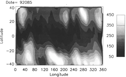
3. Satellite Emission Rate Observations

WINDII normally observed nighttime atomic oxygen green

line airglow

every

3 days

in 1992,

with an O(ID) red line day

once a week as explained in section 1. Thus we present atomic

oxygen

O(1S)

557.7-nm

emission

rate maps

for the following

nights in 1992: March 25, 28, and 31 and April 4, 7, and 14 (data were not available for the scheduled day of April 11). In Figure 5a we show the March 25 data in a form that may be directly compared with the ground-based observations, namely, vertically integrated emission rate for the atomic oxygen green line emission, plotted on a latitude longitude map for the latitude

range-40 ø- 40 ø . For this night, which is prior to both the

Stockholm and Bear Lake enhancements, we see a clearly defined equatorial minimum, characteristic of the equatorial airglow in

the postmidnight hours, as described by Shepherd et al. [1995].

At 30øN the local time is about 0240 LT, and at 30øS it is 2330 LT, while at the equator it is near 2400 LT. The minimum oscillates slightly about the equator. At higher latitudes there are prominent planetary scale structures, particularly in the southern hemisphere where they resemble wavenumber 3.

Figure 5b shows the same situation for March 28, 1992, the day of the MISU peak. The mid-latitude planetary scale patterns persist but are now more prominent in the northern hemisphere than in the southern, the opposite of what was observed 3 days earlier. The tropical emission has brightened and become a sinusoidal (wavenumber-3) emission valley, with a width of

about 15 ø and an amplitude of about 20 ø in latitude. The emission

rates at 40øN are weak, with no obvious connection to the enhancement occurring at the same time at Stockholm.

In Figure 5c for March 31 the emission rates are still low at Stockholm longitudes, but there are strong localized regions near

260

ø and 340

ø longitude.

These are east of BLO (at 212

ø) but

all signs of zonal continuity in the equatorial minimum have vanished, with bright equatorial features near the longitudes of

50 ø and 180

ø and deep depletions

near longitudes

of 240

ø and

300

ø . The latter depletion extends

to both north and south

latitudes, and near 35øN latitude it spreads longitudinally,

extending westward past Bear Lake, which agrees well with the

observation from Figure 2 that the BLO depletion is just under

way on April 4. Thus the satellite view not only confirms the ground-based observation but shows that this depletion is of

planetary scale, extending from at least 40øS to 40øN. The depletion observed duhng the same period at Stockholm may be

216 SHEPHERD ET AL.: SPRINGTIME TRANSITION IN ATOMIC OXYGEN Date- 92085

',?•..'-•':4i•...:•' .• •?• '.'" . ...

.;::",,½o

,•,,,, ..

Longitude

Figure

5a. Vertically

integrated

(zenithal)

emission

rate

for the O(1S)

558-nm

airglow

measured

by the wind

imaging

interferometer

(WINDII) for March 25, 1992.

The bar indicates

the emission

rate in rayleigh.

".•:...•a•ai

.... '.•.•.

:..:'i•.•.

::.

.(."

.iii•::;•

.4:"•ii:g.*:.-'.:!i•i;

•' •.*..':•!;•..*,.'.

....',

"$'....;

':--.•-:?

Longitude

•-½,ir•'--•,•.-...--'••

ß -;

...

.

Figure

5b. Vertically

integrated

(zenithal)

emission

rates

for the

O(•S)

558-nm

airglow

measured

by WINDII for March

28, 1992.

Date- 92091

0 40 80 120 160 200 240 280 320 360

Longitude

SHEPHERD ET AL.: SPRINGTIME TRANSITION IN ATOMIC OXYGEN 217 Date= 92095 •:•*•*•* •:::• ::::'•'• :½•.:" :•.•.•.•::':'.a .... :':'.. ;-.•'•:-:<•. :•?•a•:•;'• "½:tCt• "E"½•'•'•••. '

-- 2 0

...:'::.•'•?z•Mi?•:s•,:::

--.'::•:•j•;-::. .':•--:'-..;•:::::.

-'•.".:..

Longitude

-,:.:,.,-.,..-...-:•:....•i?

• 550

'"'!':"•!?'

i • '

250

Figure

5d. Vertically

integrated

(zenithal)

emission

rates

for the

O(1S)

558-nm

airglow

measured

by WINDII for April

4, 1992.

Date- 92098

4 0 ' '"'":'"':' ... '"'*"* "'::*":":' • ' : .... ';' ' ... ' .... *" •*"*'"•.-'"'•'-"'•" '•'

.... i..:.'•i,.:.:.:.;•i.•:•':..;½4....':•' •!•!' ":•/: .., ..,.-:•,. '.:i.-'.:•..•"":• I ..-?.?..'.; x•!•?•.;.' .•: '•{,•.:i' .?'-.: .y I

-..: •t•,,-.:: .•:•:•:-:.:.:½•.::::..::•.:..:•;;•.-..:...•.:.... , .... : ... : ... •:.:.: ... :...;:,•,.•::.:..:,, . .... z.:.•::.,..,..,•: .: ... :.:.:

"..-':.•,:.: '?,'.:'?,'.::.:½"*•--- _... :.,;..::.: _{' ...} ;:-"½...-'•a '--• ' ' ! *½...1•;:: _•':' ß .... ,t..,. "',:,. _•'•" .; _{... ,. ';} '-:'".,•:. ß •e..':.: _{•::.:t*-:-s.'.½i:½:..-'.'..'} ,::..•i:;,,a'-: _{"i",;:!i•i-"•:;} : .:*sa': • ,..,'

ß

•i'•* .,'.:.•

.'.•'.,s.':

ß

B• '•*-"?-:"""'•q•:::f"

ß

'*•:

... ß .::. ::: •.•:: ß ... •-.. ... •- .-.: .•:--'--'-• --- - ..- ... • .-'• ...•. : ... . .. ... • • o•.

o-•...,.-:.•::•.•.. (.. :,::½-..-.::•:' •.•.•-:-.. ?< .•s-..,:..,:•.,.::.::•.,.,•,%•:.:•,-,,-.s•.,'j•..-• _... --•:.• ,, .-e,• , _if2. '•. ß .•-•.•?/•_

;,-.":$'

:.'-"

?'

-'.;?.:4-'-.

' ½"*

' ,•'/•..

"½•.:':'.4•c•

½.i•.';.•';-'::•

•.{•

&'::!!•:•-J

;":.$.•:

-,'

"•-

,•';..

'•.•

-

.½•

,•;'.½.½::½.•Z.".'•'i½.*:J•-:':"4•,•?.•

•.

45O 350 25O 150 50 -40 0 40 80 120 160 200 240 280 320 360

Longitude

Figure

5e. Vertically

integrated

(zenithal)

emission

rates

for

the

O(1S)

558-nm

airglow

measured

by WINDII

for April

7, 1992.

Date- 92105

-20

-40

'•i::" '•;i .... -:•©: :'•.•;:'-".-..' ";,,½',.-*"•-' ' *'-- ;•"'" "{iF 2• '

: 0 250 150 50 I I I I I I I I 0 40 80 120 160 200 240 280 520 560

Longitude

218 SHEPHERD ET AL.: SPRINGTIME TRANSITION IN ATOMIC OXYGEN

associated with this same feature or with the smaller depletion

seen in the satellite view at 40øN and 40øE. Or perhaps these two

depletions

seen at the 40øN boundary

of the image merge

together at higher latitudes, forming a polar "hole." One cannot say from these data alone.

The sequence continues with the map for day 98 (April 7) shown in Figure 5e, in which the strong depletions have abated

and the pattern has tilted so as to become more parallel to the equator. The final image in the sequence is shown in Figure 5f,

for day 105 (April 14). Here the equatorial minimum has clearly reformed, while the brighter midlatitude regions are very patchy. In summary, as seen in the integrated emission rates, the global

springtime transition is seen as an apparent rotation from

isophotes aligned parallel to the equator to those with a primarily north-south alignment that cut across the equator and that are marked by deep depletions, with a rotation back to the parallel alignment afterwards. This is consistent with the ground-based observation of a single emission rate and temperature "pulse" over a given station.

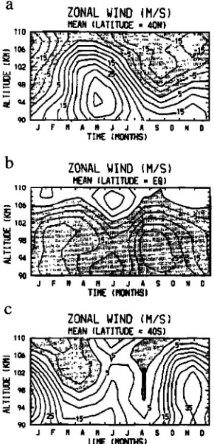
4. Wind Observations from WINDII

In Figure 6a we show the mean zonal wind determined by WINDII as a/hnction of time, averaged for the years 1992 and 1993, and as a function of altitude, for the latitude of 40øN. In January the winds are westward from 110 km (the highest altitude of data presentation) down to about 94 km. As winter

progresses toward spring, the winds reverse from westward to

eastward, with the reversal date increasing with increasing

b

ZONAL

WIND

(M/S)

MEAN l LATITUOE ß E•)

110 , , ,- ' ... J F !,t A I'1 J J A $ 0 N 0 TII• (HONTH!]I ZONAL WIND (M/S MEAN (LATITUDE: 405) 110 .'.' ,. -. ... r...:' r ... ß ...,. - , '

'::'.t.-:•..;ii!i?,:

:i:L

I•:::5, "?:'":'

J F I• A # J J A S 0 N lillE:

Figure 6. Zonal wind observed by WINDII as a function of the

month of the year for three different latitude regimes, including (a) 40øN, (b) the equator, and (c) 40øS.

ß

altitude. For the end of March the reversal altitude is at 107 km,

implying

an interaction

region

well above

the airglow

layer that

suggests

an association

with the atomic

oxygen

reservoir,

from

to note

that

the

eastward

jet whose

maximum

velocity

of 40 m s

-1

occurs at 94 km in May has no counterpart in the northern autumn. For 40øS, shown in Figure 6c, the pattern is reversed with the eastward jet peaking in altitude in November. For the equator, shown in Figure 6b, there is little seasonal variation.

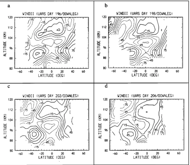
In summary, from January to March the northern hemisphere

wind reversal (westward above and eastward below) has

gradually moved up through the altitude range of observation. In Figure 7 we show the data day by day during the transition period. It must be noted that for these daily wind patterns, what is

shown is the total wind. These daily winds, with the inclusion of

instantaneous tidal components, represent the actual winds present over the ground stations, and thus more closely correspond with the behavior of the ground-based airglow observations. Figure 7a shows the zonal wind for March 25,

1992, as a function of latitude and altitude. As in the previous

averaged data, we see westward winds at the equator through the altitudes of airglow emission, and wind reversals with altitude at

midlatitudes. For the northern hemisphere the reversal is around 110 km, but the zero-wind line is tilted, so that it is at a higher

altitude at higher latitudes. By March 27, shown in Figure 7b, the reversal has moved upward so that it is eastward over the whole altitude range at 35 ø , and the tilt of the zero-wind line has

increased. For March 31, shown in Figure 7c the reversal appears

complete, with lines of constant wind near vertical. This pattern continues in Figure 7d, for April 4, but with winds of increased magnitude near 40 ø .

5. Longitudinal Variations

The emssion rate patterns of Figure 5 are complicated to interpret, so we present in Figure 8 simple line plots of volume

emission rate at a fixed altitude versus longitude for a fixed latitude band, 42 ø - 45øN, for each of the six selected days during

the 1992 transition period. In Figure 8a, day 92085 (March 25), we see a simple wavenumber 1 pattern varying roughly from t00

photons

per

cm

-3 s

-1 in the

valley

to 250

photons

per

cm

-3 s

-1 at

the peak, and in Figure 8b for March 28 the pattern is similar. However, on March 31 (Figure 8c) the pattern has dramatically altered to a kind of square-wave, with minimum values near 50

photons

per

cm

-3 s

-1 in the

European

sector

and

maxima

reaching

500

photons

per

cm

-3 s

-1 in the

North

American

sector.

By April

4 (Figure 8d) the contrast has weakened, and the pattern has shifted to put the minimum in the American sector and the maximum in the European sector, all of which is consistent with the ground-based data. By April 14 (Figure 8f) the regular wavenumber 1 pattern has been reestablished but with a

-3 s-1 and a maximum near 350

minimum near 50 photons per cm

photons

per

cm

-3 s

-1. So a depleted

region

still

exists,

near

180

ø

longitude,

a region

more depleted

than that which existed

at any

in Figure 8 the local time is shown.

During the entire

period

the

influence on the emission rates. However, during the

postmidnight

period

the effect

is not large

and so does

not unduly

SHEPHERD ET AL.: SPRINGTIME TRANSITION IN ATOMIC OXYGEN 219

latitudes, but we briefly describe what was found. At the equator

the wavenumber 1 is also evident in emission rate before the

transition with a very low valley value of about 20 photons per

cm

-3 s

-1. A planetary

scale

perturbation

is seen

during

the

transition, though it is not as large as that at midlatitudes, and

following the springtime transition, the emission rate values are

larger

than

they

were

before,

near

200

photons

per

cm

-3 s

-l. At

40øS, the emission rate is high before the transition occurs, about

300 photons

per

cm

-3 s

-1. A planetary

scale

perturbation

is seen,

and after the transition is over the emission rate is lower, around

200

photons

per

cm

-3 s

-1.

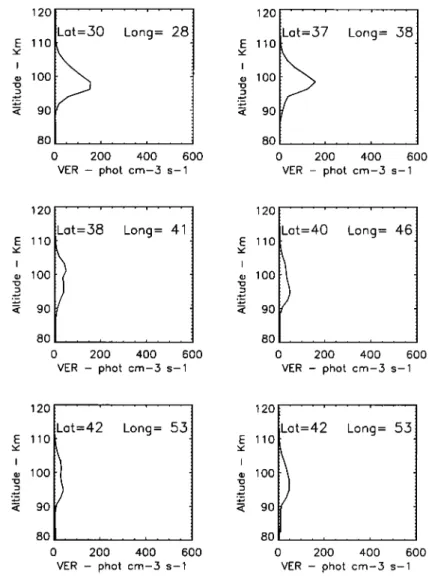
6. Evidence of Vertical Motion

The extremely large emission rate perturbations observed

require a mechanism

for this global redistribution

of atomic

perturbations

associated

with the quasi 2-day wave were the

result of vertical motions. Accordingly, the springtime transition

cannot be simply a "rotation" of the global pattern but rather a dynamical perturbation which produces large-scale planetary

structures in emission rate through strong vertical motions

leading to localized enhancements and depletions and perhaps also to a long-term temporal depletion in atomic oxygen. Support

for this hypothesis is provided by individual profiles of WINDII emission rate, shown in Figures 9a and 9b. These profiles are for March 31, 1992 (Figure 5c), the day of the maximum at Stockholm, and they consist of six successive volume emission

rate profiles taken along each of two orbit tracks four orbits apart.

The first track (Figure 9a) passes through the peak values of the

planetary scale "square wave" reaching values of 400 photons

per cm

-3 s

-1 near

310

ø longitude,

while

the second

(Figure

9b)

passes through the deep minimum that reaches 50 photons per

cm

-3 s

-1 near

40

ø longitude.

The latitudes

for each

pair

of profiles

are 30 ø, 33 ø, 38 ø, 40 ø, 41 o and 42 ø. For the first profile of Figure

9a we see for the "maximum" track a profile with a primary maximum at 93 km and a secondary maximum at 99 km; the "normal" altitude for the green line peak is 97 km. For the "minimum" track shown in Figure 9b the corresponding profile is

single and coincides in altitude and peak emission rate almost

exactly with the secondary 99-km peak of the maximum profile,

with

a peak

volume

emission

rate

of 175

photons

per cm

-3 s

-1.

That is, at 30 ø latitude the maximum profile differs from the

minimum by the addition of a second emission layer with a peak

at 93 km,

having

a peak

emission

rate

of 200

photons

per

cm

-3 s-

1. In the next

pair of profiles,

at 33

ø, the minimum

profile

has

hardly changed, while for the maximum profile the lower layer

has

strengthened

to about

230 photons

per cm

-3 s

-1 so that

its

double peak is barely evident.,.

VINOlI (UARS DAY 196/DOWNLEG) ... "l'iJ ... I: '.J' ' '/'x'/'--'x 'i ","'"';";i' ' ' ' ' -1'5 .../....' ... :...•,15

:::::::::::::::::::::::::::::::::::::

...

:"?'::"':

5/: ...

VINDII (UARS DAY 202/DOVNLEG)

' '::,:::75:?:,

:",-i!'" ....

"

ß

.:..:::'";"';:

i/...'".."?'

================================

WINDII (UARS DAY 198/00WNLEG)

f ,. &,..: ... ...--....,,,,,,, ... : .... ,.

';,,'",.,.,,:,...:...::...,

I

75 5

WINDII (UARS DAY 206/DOWNLEG)

:? .... '-';•s:::: ... / o

• 45._.

/.,.::.•

, i , , , I , , , I , , , I , , , I , , , i , , , I ,

-60 -40 -20 0 20 40 60

LATITUDE (DEG)

Figure 7. Zonal wind as a function

of altitude

and latitude

for the 4 days

of the event,

including

(a) day 196, (b)

day 198, (c) day 202, and

(d) day 206. Note the rapid

steepening

of the wind

contours

near

40øN.

220 SHEPHERD ET AL.: SPRINGTIME TRANSITION IN ATOMIC OXYGEN Loco •oo 3oo i E 2OO o o lO0

a o

200

Altitude

=9,5

d o

b o

Locol Time= 4.6 Lotitude= 42 to 45

400 ''[• ... •'-•

' • ... , ...

Altitude •95

1 oo 200 500

Longitude - Degrees

Locol Time= 2.9 Lotitude= 42 to 45

'

Altitude

E

u 200

e o

I

.AI.t!t.u.d..e.

9.5

...

, ... o

IAititude

,95 , •

Figure

8. Volume

emission

rate

(photons

per

cm

-3 s

-]) for the

OI-558

nm emission

at an altitude

of 95 km plotted

versus longitude for a latitude band 40ø-45øN for six days during the northern springtime transition of March 25 to

SHEPHERD ET AL.: SPRINGTIME TRANSITION IN ATOMIC OXYGEN 221 120 = Long=2g• 11o 100 90 80 0 200 4OO 600 VER - phot cm-3 s-1 120 = Long=299 110 100 90 80 0 2O0 400 600 VER - phot cm-3 s-1 120 110 100 90 80 ß .

=30'7

0 2OO 4OO 6OO

VER - phot cm-5 s-1 120 11o 100 90

Lot=42

Long=32'2

Figure 9a. A sequence

of volume

emission

rate profiles

taken

by WINDII along

the spacecraft

track

on March 31

near a longitude

of 300

ø. The latitude,

longitude,

and local

time for each

profile

are shown.

For the next profile, near 38 ø, there is a drastic change

between the corresponding profiles of the two tracks. For the

minimum, the peak emission rate has dropped to about 50

photons

per cm

-3 s

-1 and

become

a double

peak. The upper

of

these, at 101 km, is slightly stronger than the lower one at 95 km. For the maximum profile, the peak emission rate has almost

doubled,

to 400 photons

per cm

-3 s

-1 and

the altitude

of this

lower level peak has lowered further from 93 to 92 km. The upper

peak is just barely evident, as an inflection in the topside curve. In

the next (fourth) profile, at 40 ø , the minimum profile has

weakened further, and the lower peak is now stronger than the

upper. The maximum profile has strengthened even more, and the

next

(fifth)

profile

has

increased

to about

550 photons

per cm

-3

s

-1, while the minimum

profile

has become

single-peaked,

a

rounded curve extending to 110 km on the topside and 90 km below. From corresponding profiles that had similar peak

emission rates at 30 ø latitude, the corresponding profiles at 41 ø

latitude now have an emission rate ratio at the peak of 550/50, a factor of 11, a truly drastic perturbation. For the final pair of profiles the one on the minimum track is little changed, and the one on the maximum track has slightly weakened.

These data also show that the observed enhancements in

emission rate occur in a layer at 92 km, well below the normal

oxygen airglow altitude of 97 km. These dramatic features of Figure 9 correspond to the behavior of the springtime transition as observed at the ground-based stations. The factor-of-eleven

ratio observed by WINDII between two longitudes 90 ø apart is

about the same as that seen between the peak and depletion at Bear Lake and the other stations. These perturbations in the vertical profiles confirm strong downward motions in the enhanced regions, in which air that is rich in atomic oxygen is moved into an oxygen-poor region as described for the 2-day wave by Ward et al. [1997]. Similarly, in the depleted regions the vertical motions must be weak, or upward. Large-scale mean vertical winds have been deduced from the WINDII data by

Fauliot

et al. [ 1997]'

values

of a few cm s

-1 were

found,

in good

agreement with values determined by Portnyagin et al. [1995] from an empirical model based on ground-based wind

measurements.

7. Discussion

Space limitations preclude the presentation of data for years

additional to those shown here, but in order to confirm the regular

behavior of the springtime event, we show in Figure 10 the OI

222 SHEPHERD ET AL.: SPRINGTIME TRANSITION IN ATOMIC OXYGEN 120 11o 100 9O 8O 0 200 400 6• VER - phot cm-3 s-1 120 11o 100 9O 8O 0 200 400 600 VER - phot cm-3 s-1 120 11o lOO 90 8o 0 200 400 600 VER - phot cm-3 s-1 120 ... Lot=40 Long= 46 11o 100 90 80 ... 0 200 400 600 VER - phot cm-3 s-1 120 11o lOO 90 8o o Lot=42 Long= 53 200 400 600 VER - phot cm-3 s-1 120 11o lOO 90 8o

0 2oo 4oo 6o0

VER - phot cm-5 s-1

Figure 9b. Sequence

of profiles

as in Figure

9a, except

that

the longitude

is near

40 ø.

OHP there js a pronounced peak in the emission rate on March 29, falling 4 days later to the value existing before the enhancement. At MISU the peak is 3 days later than that for OHP; four days later, it has fallen to a value somewhat below that prior to the event, and it is then followed by a number of secondary peaks. Compared with 1992-1993, the depletion level for 1995 is not as far below that prior to the peaks as it was for

Mar20 100 I 8O 6O 40 20

Apr1Apr10Apr20 MaylMo

...

... ...

),i'•'•

MISU

- x

Day number of year

Figure 10. OI 557.7-nm emission rates at OHP and MISU for northern springtime 1995.

the earlier years. It is remarkable that the dates of the peaks for all

3 years studied here are so similar.

The peaking of emission rate as seen on the ground appears to

result from the formation of a second airglow layer near 92 km.

The coherence of the emission rate and temperature perturbations as seen from the ground points to adiabatic compression relating

to the downward motions already suggested as a mechanism.

After the peak has passed, the temperature returns, apparently reversibly, to its normal value, but the atomic oxygen remains

depleted as a result of the rapid recombination rate and the time required to replace the atomic oxygen at these altitudes. The enhanced airglow is a measure of the enhanced recombination

rate, but this visible signal is only the tip of the iceberg, as it

were, as many of the recombinations result in states that are quenched before radiation can occur. This indicates that the

drastic rise in emission rate is associated with a total loss of

atomic oxygen that is not replaced for days or even weeks. The

longer duration of the depletion at MISU as compared with that at BLO very likely reflects the longer recovery time of the atomic

oxygen at high latitudes. We recall that the hydroxyl emission did

not show a deep minimum corresponding to the oxygen

depletion. The primary excitation mechanism for the hydroxyl

emission

is as follows: O+O.2-• 0 3, followed by

H + 0 3 -->

OH*

+ 0 2 . Here

OH*

denotes

the

upper

state

of the

SHEPHERD ET AL.: SPRINGTIME TRANSITION IN ATOMIC OXYGEN 223

depleted atomic oxygen in isolation reduces the hydroxyl emission, the depletion of O is negated by another effect. The

production rate of O 3 is proportional to the product of the atomic

and molecular oxygen concentrations, so that it is plausible that with the rapid conversion of atomic to molecular oxygen associated with the emission peak, the rate of production of ozone is little changed, allowing the hydroxyl emission to return to its prior value when the adiabatic compression has passed.

The mechanism by which the wind reversal leads to the strong

vertical motions on a planetary scale deserves further investigation. Although the averaged wind data shown in Figure

6 suggests a gradual change in the wind pattern, the day-by-day

wind fields of Figure 7 show a more rapid change that corresponds closely in time to the rate of change in emission rate

as seen in the satellite and ground-based data. The drastic change in the background zonal circulation affects all the components of

the wind system. This includes the changed contribution of the

semidiurnal tide, and the reversal of the mean vertical wind from a winter-like motion (downward) to a summer-like motion

(upward).

More difficult questions are how the springtime transition as described here relates to stratospheric warmings on one hand, and on the other the stablisted equinoctial effects such as the maximum in amplitude of the diurnal tide [McLandress et al.,

1996], and the maximum in the mid-latitude airglow [Cogger et al.• 1981]. Related to this is the question of a northern hemisphere autumnal transition. While these questions remain to

be investigated, the springtime transition will likely prove to be

an important insight in the exploration of these semi-annual characteristics that are, as yet, poorly understood.

8. Conclusions

1. As observed by ground-based optical instruments, the springtime transition as observed in the northern hemisphere is characterized by the sudden rise (over a few days) in integrated emission rate for the oxygen and hydroxyl airglows by a factor of 2-3, followed by a decrease in the oxygen airglow from the peak value by a factor of 10, and a return of the hydroxyl emission to its value prior to the enhancement.

2. Airglow temperatures obtained from these emissions are

coherent with the emission rates, suggesting that the enhancement is the result of adiabatic compression of the airglow layer. The

temperature perturbations are large; for the 0 2 atmospheric band

the change is from 230 to 163 K in a period of just 4 days.

3. The global integrated emission rate pattern observed by

WINDII shows isophotes that are aligned parallel to the equator prior to the transition, with an equatorial minimum, and these

isophotes rotate to become nearly parallel to the meridian,

returning to an equatorial alignment again afterward.

4. The satellite and ground-based views are consistent in that

at a ground-based site the enhancement appears as a pulse that

passes a given ground station only once. Specific comparisons of the satellite and ground-based data agree well.

5. Plots of longitudinal variation show the transition pulse as a large planetary-scale feature (wavenumber 1) with extremely large peak-to-valley ratios, of about 10.

6. WINDII emission rate profiles show that these planetary scale features are accompanied by strong vertical motions; the emission rate enhancement is manifested in the formation of a second emission layer at about 92 km.

7. These strong downward motions indicate a rapid conversion of atomic to molecular oxygen, which is not immediately reversible, causing the long-term depletion following the

transition. The enhanced WINDII emission rate profiles are consistent with the enhancements of ground-based observations

of the oxygen and hydroxyl airglows.

8. The WINDII wind measurements suggest that this emission rate perturbation is associated with the springtime wind reversal, in which the altitude of reversal rises gradually to some critical altitude. At the same time, the slope of the latitudinal wind

gradient rapidly steepens.

9. The springtime transition as described here appears to be just part of the entire global picture of the dynamics of the semi- annual variation of the lower thermosphere, which deserves a

more cornprehensive investigation.

Acknowledgments. The WINDII project is sponsored by the

Canadian Space Agency and the Centre National d'Etudes Spatiales of France and supported by the Natural Sciences and Engineering Research Council of Canada.

Janet G. Luhmann thanks David Rees and another referee for their

assistance in evaluating this paper.

References

Cogger, L.L., R.D. Elphinstone, and J.S. Murphree, Temporal and

latitudinal 5577 A airglow variations, Can..I. Phys., 59, 1296-1307,

1981.

Fauliot, V., G. Thuillier and F. Vial, Mean vertical wind in the

mesosphere-lower thermosphere region (80- 120 km) deduced from

the WINDII observations on board UARS, Ann. Geophys., 15, 1221- 1231, 1997.

Gault,

W.A.,

et al., Validation

of O(1S)

wind

measurements

by WINDII:

The WIND imaging interferometer on UARS, J. Geophys. Res., 101,

!0,431-10,440, 1996.

McLandress, C., G.G. Shepherd, and B.H. Solheim, Satellite

observations of thermospheric tides: Results from the wind imaging

interferometer on UARS, J. Geophys. Res., 101, 4093-4114, 1996. Portnyagin, Y. I., J.M. Forbes, T.V. Solovjeva, S. Miyahara, and C.

DeLuca, Momentum and heat sources of the mesosphere and lower thermosphere regions 70 - 110 km, J. Atmos. Terr. Phys., 57, 967-977,

1995.

Shepherd, G.G. et al., WINDII: The wind imaging interferometer on the

upper atmosphere research satellite, J. Geophys. Res., 98, 10,725-

10,750. 1993.

Shepherd, G.G., C. McLandress and B.H. Solheim, Tidal influence on

O(lS)

airglow

emission

rate

distributions

at the

geographic

equator

as

observed by WINDII, Geophys. Res. Lett., 22, 275-278, 1995.

Stegman, J., D. Murtagh and G. Witt, Extremes of oxygen airglow intensity (abstract), Eos Trans. 73(14), AGU, Spring Meeting Suppl.,

S222, 1992.

Thuillier, G., V. Fauliot, M. Herse, L. Bourg, and G.G. Shepherd, MICADO wind measurements from Observatoire de Haute-Provence for the validation of WINDII green line data, J. Geophys. Res., 101,

10,431-10,440, 1996.

Ward, W.E., B.H. Solheim, and G.G. Shepherd, Two day wave induced

variations in the oxygen green line volume emission rate: WINDII observations, Geophys. Res. Lett., 24, 1127-1130, 1997.

Wiens, R.H., S.P. Zhang, R.N. Peterson, and G.G. Shepherd, MORTI: A mesopause oxygen rotational temperature imager, Planet. Space

Sci., 39, 1361-1375, 1991.

Wiens, R.H., S.-P. Zhang, R.N. Peterson, and G.G. Shepherd, Tides in

emission rate and temperature from the 02 nightglow over Bear Lake

Observatory, Geophys. Res. Lett. 22, 2637-2640, 1995.

P. Espy, Embry-Riddle Aeronautical University, Daytona Beach, FL

32114-3900.

C. McLandress, G.G. Shepherd, and R. H. Wiens, Centre for Research in Earth and Space Science, York University, 4700 Keele Street, Toronto, ON, Canada, M3J 1P3. ([email protected])

J. Stegman, Arrenius Laboratory, Stockholm University, Stockholm,

S-106 91, Sweden.

G. Thuillier, Service d'Atronomie, B.P. No. 3, 91371 Verri•res-le- Buisson CEDEX, France.

(Received May 11, 1998; revised August 20, 1998;