HAL Id: hal-00297684
https://hal.archives-ouvertes.fr/hal-00297684
Submitted on 10 Apr 2008
HAL is a multi-disciplinary open access
archive for the deposit and dissemination of
sci-entific research documents, whether they are
pub-lished or not. The documents may come from
teaching and research institutions in France or
abroad, or from public or private research centers.
L’archive ouverte pluridisciplinaire HAL, est
destinée au dépôt et à la diffusion de documents
scientifiques de niveau recherche, publiés ou non,
émanant des établissements d’enseignement et de
recherche français ou étrangers, des laboratoires
publics ou privés.
M in the Norwegian Sea
I. Skjelvan, E. Falck, F. Rey, S. B. Kringstad
To cite this version:
I. Skjelvan, E. Falck, F. Rey, S. B. Kringstad. Inorganic carbon time series at Ocean Weather Station
M in the Norwegian Sea. Biogeosciences, European Geosciences Union, 2008, 5 (2), pp.549-560.
�hal-00297684�
www.biogeosciences.net/5/549/2008/
© Author(s) 2008. This work is distributed under the Creative Commons Attribution 3.0 License.
Biogeosciences
Inorganic carbon time series at Ocean Weather Station M in the
Norwegian Sea
I. Skjelvan1,2, E. Falck2, F. Rey3, and S. B. Kringstad2,1
1Bjerknes Centre for Climate Research, University of Bergen, Norway 2Geophysical Institute, University of Bergen, Norway
3Institute of Marine Research, Bergen, Norway
Received: 15 August 2007 – Published in Biogeosciences Discuss.: 27 August 2007 Revised: 18 February 2008 – Accepted: 18 March 2008 – Published: 10 April 2008
Abstract. Dissolved inorganic carbon (CT) has been
col-lected at Ocean Weather Station M (OWSM) in the Norwe-gian Sea since 2001. Seasonal variations in CT are confined
to the upper 50 m, where the biology is active, and below this layer no clear seasonal signal is seen. From winter to sum-mer the surface CT concentration typical drop from 2140 to
about 2040 µmol kg−1, while a deep water CT concentration
of about 2163 µmol kg−1is measured throughout the year. Observations show an annual increase in salinity normalized carbon concentration (nCT) of 1.3 ±0.7 µmol kg−1yr−1 in
the surface layer, which is equivalent to a pCO2increase of 2.6 ±1.2 µatm yr−1, i.e. larger than the atmospheric increase in this area (2.1 ±0.2 µatm yr−1). Observations also show an annual increase in the deep water nCT of 0.57±0.24 µmol
kg−1yr−1, of which about 15% is due to inflow of old Arc-tic water with larger amounts of remineralised matter. The remaining part has an anthropogenic origin and sources for this might be Greenland Sea surface water, Iceland Sea sur-face water, and/or recirculated Atlantic Water. By using an extended multi linear regression method (eMLR) it is veri-fied that anthropogenic carbon has entered the whole water column at OWSM.
1 Introduction
The ocean is one of several reservoirs indirectly controlling the climate system through exchange of CO2 with the at-mosphere. Human activities, such as burning of fossil fu-els and deforestation, release annually an anthropogenic car-bon amount of about 7.2×10¹⁵g C into the atmosphere, and of this, about one third is taken up by the world oceans (Solomon et al., 2007). The North Atlantic is known to store relatively large amounts of anthropogenic carbon, which has
Correspondence to: I. Skjelvan ([email protected])
been captured through formation of intermediate and deep waters in subpolar areas (e.g. ´Alvarez et al. 2003; Friis et al., 2005; Olsen et al., 2006). It is, however, not straight-forward to quantify this amount, due to a lack of oceanic reference data from the pre-industrial times, and alternative methods have to be used, such as back-calculation techniques (e.g. Brewer, 1978; Chen and Millero, 1979; Gruber et al., 1996) or empirical methods (Wallace, 1995; Goyet et al., 1999; Friis et al., 2005).
The Nordic Seas in the North Atlantic are an important sink for atmospheric CO2(e.g. Takahashi et al., 2002; Skjel-van et al., 2005). Takahashi et al. (2002) pointed out that the size of the sink is increasing due to an unchanged sur-face ocean pCO2signal in this area over the years. Recent research suggests, on the contrary, that the size of the Nordic Seas sink seems to be regionally decreasing, based on an ob-served seawater pCO2which annually increases faster than the atmospheric pCO2(Olsen et al., 2006). Carbon time se-ries data from this area are, in this respect, valuable contri-butions to evaluate the development of the oceanic carbon uptake.
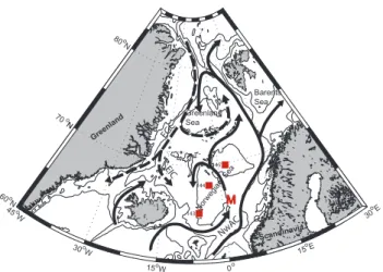
The Ocean Weather Station M (OWSM) is situated in the western branch of the Norwegian Atlantic Current, at 66◦N; 2◦E, over the Norwegian continental slope (Fig. 1). The sta-tion, which has a depth of about 2100 m, was started in 1948 and is today operated by M/S Polarfront; the last weather ship in the world. Temperature and salinity have been mea-sured from the very beginning (e.g. Østerhus and Gam-melsrød, 1999; Nilsen and Falck, 2006), closely followed by dissolved oxygen (Nilsen and Falck, 2006; Kivim¨ae and Falck, 20071). In the 1980s analyses of atmospheric CO2 content were started (Tans and Conway, 2005), and since 1990 nutrients have been determined weekly (Dale et al., 1999). During a four years period and on a monthly basis in the early 1990s, total dissolved inorganic carbon (CT) was
1Kivim¨ae, C and Falck, E.: Interannual variability of net
com-munity production at Ocean Weather Station M in the Norwegian Sea during 51 years, Global Biogeochem. Cy., submitted 2007.
45o W 30o W 15o W 0o 15 oE 30 oE 60o N 70o N 80o N Greenland Sea M EGC NwA C EIC Barents Sea 143 144 145 Norw egia n Se a Gre enla nd Scandin avia
Fig. 1. Schematic of the northern North Atlantic Ocean. The solid
lines indicate the flow of warm Atlantic Water and the dashed lines show the flow of cold Polar and Arctic Water. NwAC is the Nor-wegian Atlantic Current, EGC is the East Greenland Current, and EIC is the East Icelandic Current. M denotes Ocean Weather Sta-tion M (OWSM) and the red squares indicate TTO staSta-tions used for estimating anthropogenic carbon increase at OWSM.
determined for the very first time at OWSM, using gas ex-traction of acidified water samples and manometric detec-tion (Gislefoss et al., 1998), however, these are not used in the following due to insufficient precision (±12 µmol kg−1). Since November 2001 monthly measurements of CT have
been performed using modern analyzing techniques. Warm and saline Atlantic Water from the Norwegian At-lantic Current occupies the upper layer at OWSM down to 300–400 m, with present temperatures typically varying between 7◦C in the winter and 12◦C in the summer time (Fig. 2a). Cold and less saline deep water occupies the water column from about 1000 m down to the bottom (Norwegian Sea Deep Water), and in between these two water masses there is a layer of intermediate water; Arctic Intermediate Water, of fluctuating thickness. At times with northerly or north-easterly winds during summer, the fresher Norwegian Coastal Water is driven away from the coast and will occa-sionally reach all the way out to OWSM (Fig. 2b). We refer to Nilsen and Falck (2006) for a more thorough description of the hydrographic conditions in the OWSM area.
In this paper we present the new CT time series data from
OWSM in the Norwegian Sea since fall 2001. We describe the seasonal and interannual variations, and we use the multi-ple linear regression (MLR) method of Wallace (1995) in an extended version (eMLR) formalized by Friis et al. (2005) to determine the anthropogenic CO2increase in this area of the Nordic Seas during the last two decades since the Tran-sient Tracers in the Ocean, North Atlantic Study (TTO-NAS) expedition in 1981.
2 Data
At present, hydrographic measurements at OWSM are per-formed using a Sea-Bird CTD (SBE 37-SM MicroCAT with conductivity, temperature, and pressure sensors), which is calibrated towards bottle salinity samples. Nansen bottles, with reversing thermometers, are used to collect samples for inorganic carbon, dissolved oxygen, nutrients, and salinity at standard depths. Samples for CT are conserved with 0.02%,
by volume, of saturated HgCl2solution and analysed ashore in general within a month. However, a few samples have been stored for up to six months when the analytical instru-ments have been occupied at cruises. CT is determined by
gas extraction of acidified water samples and further coulo-metric titration (Johnson et al., 1993; DOE, 1994), and accu-racy is set by running CRM supplied by Andrew Dickson of Scripps Institution of Oceanography. The precision (standard deviation) is ±0.5 µmol kg−1 based on 10 duplicate sam-ples. Dissolved oxygen is measured on board using the Win-kler titration method with visual detection of the titration end point, and this in general gives a precision of 1%. Nutrients are conserved using chloroform and kept at 4◦C until anal-ysis ashore within six weeks after sampling. The analyses were made using standard methods on a Skalar Auto Ana-lyzer until 2003 and an Alpkem Auto AnaAna-lyzer since then. Precision for nitrate, phosphate, and silicate are 3%, 4%, and 2%, respectively. The salinity samples are analyzed ashore within a month after sampling using PorterSal salinometer with a precision of 0.003. Due to technical problems there is a gap in the time series from April to October 2004, i.e. no water samples were collected during this period.
The TTO-NAS ran from April to October 1981 and con-sisted of 7 legs. In the present study we have used data from leg 5, which was carried out during July and August 1981 in the Nordic Seas, and the precision of the inorganic car-bon data from this cruise is reported to be ±3.7 µmol kg−1. The data were obtained from the Carbon Dioxide Informa-tion Analysis Center (Oak Ridge, Tennessee, USA) and are thoroughly described in e.g. Olsen et al. (2006). Tanhua and Wallace (2005) reanalyzed TTO carbon data from legs 2, 3, 4, and 7, and compared them with modern data adjusted to CRMs. They concluded that the TTO alkalinity data were bi-ased and recommended that these data should be reduced by 3.6 µmol kg−1, and that the TTO CT data should be
recalcu-lated using adjusted alkalinity data and further increased by 2.4 µmol kg−1. No significant leg-specific differences were found for the four legs examined, and based on this the sug-gested corrections have also been performed on the data from leg 5.
3 Seasonal and interannual variability
The inorganic carbon content of the seawater in this area varies at different time scales. The upper water mass at
Fig. 2. Hovm¨oller diagram of water column (a) temperature [◦C] and mixed layer depth (white line), (b) salinity, (c) CT [µmol kg−1], (d)
-2 0 2 4 6 8 10 12 14 2001 2002 2003 2004 2005 2006 2007 T e m p e ra tu re [ oC ] a 34.8 34.9 35.0 35.1 35.2 35.3 35.4 2001 2002 2003 2004 2005 2006 2007 S a li n it y b 2020 2060 2100 2140 2180 2001 2002 2003 2004 2005 2006 2007 C T [µ m o l kg -1 ] c 0 4 8 12 16 2001 2002 2003 2004 2005 2006 2007 N it ra te [ µ m o l kg -1 ] d 0 4 8 12 2001 2002 2003 2004 2005 2006 2007 S il ica te [ µ m o l kg -1 ] e
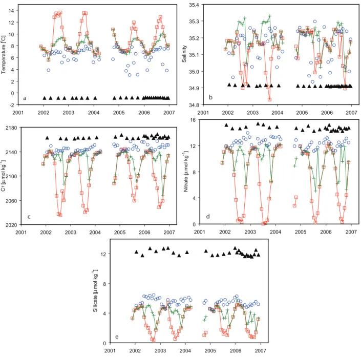
Fig. 3. Seasonal variations in (a) temperature, (b) salinity, (c) CT, (d) nitrate, and (e) silicate at different depths as a function of time. Red
squares are at 10 m, green crosses are at 50 m, blue circles are at 200 m, and black filled triangles are at 2000 m depth.
OWSM experiences seasonal changes due to physical, chem-ical, and biological processes. A clear seasonality is, for instance, seen in the upper layer temperature with warm-ing durwarm-ing the summer seasons and coolwarm-ing durwarm-ing winters (Fig. 2a). The depth of the mixed layer at OWSM varies in general between 20 m in summer to 250–350 m in win-ter (Fig. 2a) and below the winwin-ter mixed layer no clear sea-sonal signal is seen. For the current work the mixed layer depth (Fig. 2a) was determined as the depth where the σt
had changed equivalent to a decrease in the surface temper-ature of 0.8◦C (Kara et al., 2000). For density profiles with
surface instability stronger than 0.02 kg m−3, the first stable value below the surface was used as the surface value.
The depth of the transition layer between the Atlantic Wa-ter and the inWa-termediate waWa-ter at OWSM is known to fluctu-ate considerably (e.g. Mosby, 1962) and this can clearly be seen in Fig. 2a at depths between 300 and 600 m, where the period of the temperature fluctuations is disconnected with the season. Below about 700 m the temperature decreases toward the bottom from 0 to about –0.83◦C.
Panel 2c, d, and e show all the CT, nitrate, and silicate data
CT, nitrate, and silicate are extracted at four depths. The
highest variability for all parameters is seen in the surface layer, and this is closely linked to the biological activity start-ing in the sprstart-ing and extendstart-ing into the summer season. Phy-toplankton growth starts in April-May as a combined result of increased solar radiation, shallowing of the mixed layer, and the establishment of a seasonal pycnocline (Rey, 2004). With the onset of primary production the concentrations of CT and nutrients decrease in the surface layer. This
deple-tion continues until mid or late summer, when respiradeple-tion and remineralisation take over as dominating processes control-ling the CT and nutrients concentrations.
At 50 m depth there is a temporary decrease in CT,
ni-trate, and silicate concentrations just after the onset of pri-mary production, when the mixed layer is still deeper than 50 m. The major depletion at this depth appears to occur in September-October (Fig. 3c, d, and e), when the surface wa-ter low in CT and nutrients is mixed downwards due to wind
mixing and vertical convection achieved by cooling of the surface (Fig. 3a). As the mixed layer depth increases further the carbon and nutrient rich waters from depths below 50 m are mixed upwards in the water column and reintroduced into the surface layer, increasing the surface concentrations towards winter values.
The biological drawdown during spring and summer is confined to the upper 50 m and below 100 m there is no clear seasonal signal in CT and nutrients. From winter to summer
the surface CT, nitrate, and silicate decrease by about 100,
11, and 4 µmol kg−1, respectively (Fig. 3c, d, and e). The lowest surface CT concentrations are found in August, while
the nutrients have their lowest concentrations in July. While there is an indisputable difference between summer and winter values in upper waters, no clear seasonal signal is seen in the deeper layers. In the transition zone between the Atlantic Water and the Arctic Intermediate Water (300– 600 m; Fig. 2c) the CT concentration increases from about
2140 to about 2165 µmol kg−1. In the core of the interme-diate water, between about 500 and 1000 m, there is a small CT maximum, and below this the concentration is slightly
decreasing towards the bottom. For nitrate (Fig. 2d), the increase in the transition layer is about 2 µmol kg−1, with a small further increase of 1 µmol kg−1in the deep water. The silicate concentration (Fig. 2e) increases from about 6 to about 8 µmol kg−1 in the transition zone, and increases further towards the bottom. At 2000 m depth CT, nitrate,
and silicate values are about 2163, 15, and 12 µmol kg−1, respectively, throughout the year. Typical values for the dif-ferent parameters at difdif-ferent depth layers and seasons are presented in Table 1, however, deviations from these are cer-tainly observed.
When it comes to interannual variations, the degree of inorganic carbon depletion in the mixed layer during sum-mer seasons do vary from year to year; a feature which is also seen in the silicate, but not in the nitrate (Fig. 3c, d, and e). In 2005, the concentration of CT dropped by about
2120 2125 2130 2135 2140 2145 2150 2001 2002 2003 2004 2005 2006 2007 n C T [µ m o l kg -1 ] a 2120 2125 2130 2135 2140 2145 2150 2001 2002 2003 2004 2005 2006 2007 n C T [µ m o l kg -1 ] b 2150 2155 2160 2165 2170 2175 2001 2002 2003 2004 2005 2006 2007 n C T [µ m o l kg -1 ] c
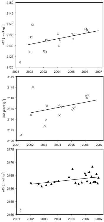
Fig. 4. Salinity normalized carbon concentration over the period
2002–2006 in (a) the surface water during the winter months uary to March, (b) the mixed layer during the winter months Jan-uary to March, and (c) the deep water (four times a year in 2002– 2004, and once a month from 2005 and onwards). The surface CT
samples are normalized to a salinity of 35.1, while the deep water samples are normalized to a salinity of 34.91. Equations, number of data points, R2, and significance level for the different regression lines are for (a) y=1.28·x–431, 15, 0.22, and 92%; for (b) y=1.25·x– 361, 14, 0.13, and 80%; and for (c) y=0.57·x+1026, 26, 0.19, and 98%.
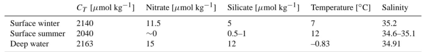
Table 1. Mean values of CT, nitrate, silicate, temperature, and salinity at OWSM.
CT [µmol kg−1] Nitrate [µmol kg−1] Silicate [µmol kg−1] Temperature [◦C] Salinity
Surface winter 2140 11.5 5 7 35.2
Surface summer 2040 ∼0 0.5–1 12 34.6–35.1
Deep water 2163 15 12 –0.83 34.91
80 µmol kg−1 from winter to summer compared to a CT
drop of about 100 µmol kg−1from winter to summer in pre-vious years. A similar picture is seen for the salinity nor-malized CT (nCT=CT·S/35.1; not shown), which indicates
that this feature is not caused by a change in salinity. The feature is mainly explained by a colder surface temperature during summer 2005 compared to the previous summers (see Figs. 2a and 3a). During 2005 the surface temperature was about 2◦C colder than previous years, and this corresponds to a CT increase of about 16 µmol kg−1 (Lewis and
Wal-lace, 1998). Also surface silicate values were less depleted during summer 2005 and 2006 compared to previous sum-mers. The reason for this might be connected to sub-optimal diatom growth or to heavy grazing on diatoms resulting in a lower phytoplankton biomass (Rey, 2004).
To determine the interannual trend in the inorganic carbon content of surface water, the winter surface (10 m) nCT
con-centration during the years 2002 to 2006 is plotted in Fig. 4a. Winter is defined as the months January to March, and a re-gression line is drawn through the points. The figure shows two things; first, within the same winter the mixed layer in general increases from January towards March, which in-creases the inorganic carbon concentration in the surface layer. Second, and most interesting when it comes to vari-ations from year to year, the slope of the regression line in-dicates an annual nCT increase of 1.3±0.7 µmol kg−1yr−1
(with a significance level of 92%). An annual increase of not salinity normalized CT values of 1.5±0.5 µmol kg−1yr−1
was also determined (not shown), which indicates that less than a tenth of the observed annual increase in surface CT is
due to salinity changes. The slope is equivalent to a pCO2 in-crease of 2.6±1.2 µatm yr−1assuming a constant alkalinity of 2320 µmol kg−1 (Lewis and Wallace, 1998). The win-ter season was chosen to eliminate any inwin-terannual variations due to change in primary production.
The robustness of the interannual signal was investigated by examining the inorganic carbon content in the winter (Jan-uary to March) mixed layer over the years, since the winter is the time of the year when the mixed layer is deepest and cold-est (Nilsen and Falck, 2006). Further, the salinity normalized CT content during the winter months were calculated by
inte-grating nCT throughout the mixed layer (Fig. 4b). The slope
of the regression line indicates an increase in the mixed layer nCT content of 1.2±0.9 µmol kg−1 yr−1, equivalent to an
annual pCO2increase of 2.4±1.6 µatm yr−1if one assumes
a constant alkalinity of 2320 µmol kg−1 (Lewis and Wal-lace, 1998); i.e. lower than the increase in oceanic pCO2. According to Tans and Conway (2005) and T. Conway (per-sonal communication) the annual atmospheric CO2increase at OWSM was 2.1±0.2 µatm yr−1 for the period between 2001 and 2005, and 1.63±0.03 µatm yr−1for the period be-tween 1982 to 2005; i.e. less compared to the oceanic pCO2 increase.
At intermediate depths of 800, 1000, and 1500 m we ob-serve annual increases in nCT of 1.4, 0.8 and 0.9 µmol
kg−1yr−1, respectively. Further, the water at 2000 m depth (Fig. 4c) also shows an interannual CT signal, and here the
nCT is observed to increase by 0.57±0.24 µmol kg−1 yr−1
(significance level of 97%). This might be connected to the changes seen in the deep water at OWSM during the last decades (Østerhus and Gammelsrød, 1999) and will be dis-cussed further in Chapter 5.
4 Determining changes in anthropogenic carbon
During the last decades there have been numerous attempts to determine the anthropogenic part of the inorganic carbon ex-change between the atmosphere and the ocean (e.g. Brewer, 1978; Wallace, 1995; Gruber et al., 1996; Sabine et al., 1999). In this work we have used the extended multi linear regression (eMLR) method documented in Friis et al. (2005) and based on the multivariate time-series method used in Wallace (1995) and Brewer et al. (1995), to determine changes in the anthropogenic carbon content of the water.
This method is based on the assumptions that the spatial CT distribution in a given region can be described by a
lin-ear multi-parameter model and that, over the time period of the study, there are no temporal changes in the correla-tion between CT and the independent parameters used in the
method. In the real world, CT is perturbed both by
natu-ral variability and anthropogenic input, but it is assumed that when predictive parameters such as salinity, nutrients, AOU (apparent oxygen utilization), or alkalinity are taken into ac-count this can adjust for the natural variations.
The rationale is to use a recent data set from one region; in this case OWSM data from 2005, and compare it with a historical data set from the same region; i.e. data from the TTO-NAS expedition in 1981. CT values from the two time
parameters; salinity, nitrate, silicate, and potential temper-ature, from the respective time periods:
CtT ,pred=at+btSt+ctNO3t+dtSiO2t +etθt (1)
where a, b, c, d, and e are regression coefficients specific for the particular dataset, and t refers to the TTO or OWSM data. The change of anthropogenic carbon in the water col-umn over the time span is then determined by subtracting the time specific equations from each other:
1CantT =(at 2−at 1) + (bt 2−bt 1)St 2+(ct 2−ct 1) NOt 23 +(dt 2−dt 1)SiOt 22 +(et 2−et 1)θt 2 (2)
where t1 and t2 represents the TTO and OWSM data, re-spectively. An advantage of the eMLR approach compared to the MLR is that the measurement error of the independent parameters is minimized since this error is included in the prediction both in the recent and the historical dataset (Friis et al., 2005).
With the view of the Norwegian Sea as a diatom domi-nated area, it makes sense that silicate is one of the param-eters that should be included in the predictive term for CT.
On the other hand, parameters like phosphate and AOU were also considered in the regression, with not as good fit as with the present combination of parameters. The use of phosphate and AOU even resulted in CT residuals with a biased
varia-tion with depth, which indicates that these parameters are not independent.
Three stations with hydrographical characteristics similar to those found at OWSM were selected from leg 5 of TTO-NAS (Fig. 1). These data were chosen due to relatively sim-ilar hydrographical characteristics to those found at OWSM (see Fig. 5). Nitrate values lower than 0.5 µmol kg−1, which were the case for a few data points, have been excluded in both datasets to avoid situations with possible overconsump-tion of carbon at low nutrient levels (Falck and Anderson, 2005). Table 2 provides the main outputs of the calculation. The calculated CT residuals (CT measured– CT predicted) from
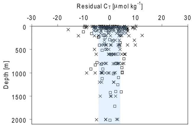
the two datasets were relatively homogenously distributed around zero throughout the water column (Fig. 6), which support the choice of independent variables for the CT
pre-diction. The highest scatter is found in the surface layer, an area of high biological activity, which suggests that the method does not fully compensate for the biology. The dis-tribution of the CT residuals is used to estimate the precision
of the eMLR method, which is determined to be ±7 µmol kg−1in the upper 200 m and ±4 µmol kg−1below 200 m.
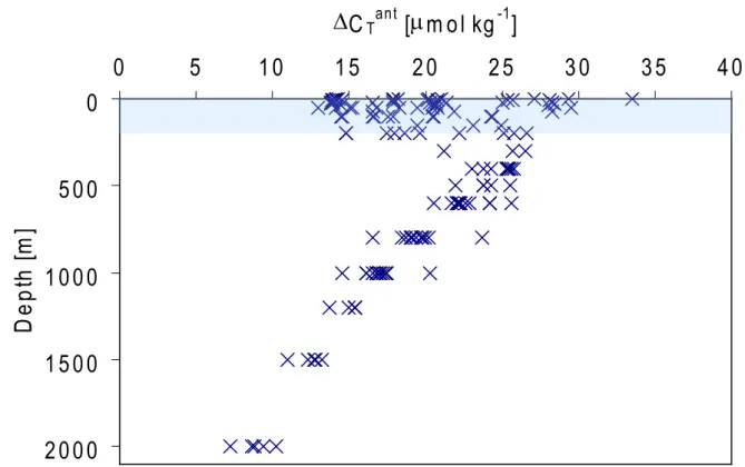
Figure 7 presents the anthropogenic increase of inorganic carbon at OWSM in the Norwegian Sea over the 24 years pe-riod from 1981 to 2005. The variation in the surface layer is large but the overall picture is that anthropogenic carbon seems to have entered the whole water column during these 24 years. The deep layer (2000 m) experienced a low anthro-pogenic carbon increase of 9 ±4 µmol kg−1, and the anthro-pogenic carbon content of the upper water mass (200–400 m)
-2 0 2 4 6 8 1 0 1 2 1 4 3 4 .8 3 4 .9 3 5 3 5 .1 3 5 .2 3 5 .3 3 5 .4 S alinity T e m p e ra tu re [ o C ] TTO 143 TTO 144 TTO 145 OW SM 2005 Surface water Deep water a -2 0 2 4 6 8 1 0 1 2 1 4 0 3 6 9 1 2 1 5 S ilic ate [µm ol kg-1 ] T h e ta [ o C ] TTO 143 TTO 144 TTO 145 OW SM 2005 ca 100 m b
Fig. 5. (a) Temperature vs. salinity and (b) theta (potential
tem-perature) vs. silicate, based on data from TTO-NAS stations 1981 (different blue symbols, see Fig. 1) and OWSM 2005 (red crosses).
increased by 25±7 µmol kg−1. These values translate to an-nual rates of about 0.4 and 1 µmol kg−1yr−1, respectively at 2000 m and 200–400 m.
The eMLR method was checked by using Eq. 2 to back-ward calculate the 1C,antT , i.e. regression constants for TTO data subtracted from regression constants for OWSM data and further multiplied with TTO data. This showed an an-thropogenic carbon increase similar to Fig. 7, which confirms the solidity of the eMLR method.
OWSM data from 2006 were also tried out in the an-thropogenic carbon change calculation, but due to unrealis-tic fluctuations and bias in the surface anthropogenic carbon values these data were not used further in the eMLR calcula-tions.
The number of anthropogenic carbon estimates in this area is scarce. Olsen et al. (2006) used a similar approach for esti-mating anthropogenic inorganic carbon content at a location west of OWSM, and they reported increases of the surface and deep waters of about 0.8 and 0.3 µmol kg−1 yr−1, re-spectively, which is slightly less than the increases reported in the present study.
Chen et al. (1990) and Anderson et al. (2000) estimated anthropogenic carbon signals for the Greenland Sea Deep
Table 2. Parameters and coefficients of Eq. 1 for the two different datasets TTO-NAS (1981) and OWSM (2005) determined from the eMLR
approach, and statistics connected to the predicted CT.
Salinity Nitrate Silicate θ
a b c d e σ R2 n
TTO-NAS –1441.67 101.55 3.31 –0.20 –6.65 4.12 0.99 85 OWSM 524.52 45.88 4.66 –2.88 –5.41 5.63 0.95 162
θ is the potential temperature.
a, b, c, d, and e are regression coefficients specific for the particular dataset.
σ , R2, and n are the standard deviation, the coefficient of determination, and the number of data points used, respectively.
0
5 0 0
1 0 0 0
1 5 0 0
2 0 0 0
-3 0
-2 0
-1 0
0
1 0
2 0
3 0
R e s id ual C
T[µm ol kg
-1]
D
e
p
th
[
m
]
Fig. 6. Residuals of CT (measured minus predicted value) as a function of depth; TTO-NAS 1981 (squares) and at OWSM 2005 (crosses).
The shaded area indicates the accuracy of the eMLR method of ±7 µmol kg−1in the upper 200 m and ±4 µmol kg−1in the deeper layers.
Water of ∼10 µmol kg−1 in 1982 and ∼15 µmol kg−1 in 1994, respectively. This corresponds to an annual increase of 0.4 µmol kg−1, which is comparable to the annual increase in anthropogenic carbon estimated for the OWSM deep wa-ter in the present study. However, it is difficult to dewa-termine any annual rate of anthropogenic change in the Greenland Sea since this depends on the strength of the deep convection which varies from year to year.
5 Discussion
The results show that over the years of this study the amount of inorganic carbon has increased in the entire water column
at OWSM, and the increase has been largest in the surface mixed layer, and least, but still significant, in the deep water. 5.1 Surface mixed layer
The surface layer (10 m) and the mixed layer nCT show
in-creases of 1.3±0.7 µmol kg−1yr−1and 1.2±0.9 µmol kg−1 yr−1, respectively, and the eMLR estimate of anthropogenic carbon verifies the observed mixed layer inorganic carbon content. The anthropogenic increase of the mixed layer (ex-cluding the surface water, where the method seems to be least accurate) is estimated to be about 25 µmol kg−1 during a period of 24 years (Fig. 7), which equals an annual CT
0
5 0 0
1 0 0 0
1 5 0 0
2 0 0 0
0
5
1 0
1 5
2 0
2 5
3 0
3 5
4 0
∆C
Tant[
µm ol kg
-1]
D
e
p
th
[
m
]
Fig. 7. Amount of anthropogenic carbon entered into the water column at OWSM from 1981 to 2005. The shaded area indicates that in the
upper waters the method is less accurate than deeper in the water column.
the eMLR method, in spite of the large standard deviation, is describing the observed situation for the water in the mixed layer.
The annual surface CT increase corresponds to a pCO2 of 2.6±1.2 µatm yr−1 (Lewis and Wallace, 1998) which is slightly higher than the rate of atmospheric CO2 increase (2.1±0.2 µatm yr−1) over the years 2001 to 2006. This is in concert with recent research (e.g. Olsen et al., 2006; Omar and Olsen, 2006) and shows that the oceanic uptake of atmo-spheric CO2in this area is decreasing. The carbon content of the Atlantic Water seems to be moving towards equilib-rium with respect to air-sea CO2exchange, and may there-fore in the future become a source of CO2to the atmosphere rather than a sink. This is intuitively in contradiction to an atmosphere with an increasing amount of CO2. However, according to Wallace (2001) this can be explained by a duced buffer capacity of the northward flowing water as a re-sult of a reduced out-gassing at lower latitudes due to higher atmospheric CO2 levels. In this way more carbon is left in the water to be transported northwards, and when the water cools on its way towards the Nordic Seas less atmospheric carbon, compared to pre-industrial times, is absorbed in the water. This is also verified by Anderson and Olsen (2002), who showed, using a simple advective model, that lower lati-tudes have the largest uptake of anthropogenic CO2from the atmosphere.
5.2 Intermediate layer
The largest increase in nCT (1.4 µmol kg−1 yr−1) is
ob-served in the intermediate layer, at 800 m depth. This water has its origin in the Greenland Sea and/or Iceland Sea (Blind-heim and Rey, 2004), where it has received its anthropogenic carbon signature in the surface water before subduction. The observed annual increase in CT at this level is compared with
the eMLR estimate, and the latter is about 19 µmol kg−1, or 0.8 µmol kg−1yr−1, which then would explain nearly 60% of the observed CT increase.
5.3 Deep layer
For the OWSM deep water, an inorganic carbon increase of 0.57±0.24 µmol kg−1yr−1is observed based on data from 2001 to 2006. This is more than the anthropogenic CT
in-crease estimated from the eMLR analysis; about 0.4 µmol kg−1yr−1, however the numbers are small and conclusions should be drawn with care.
Part of the observed deep water inorganic carbon increase might be due to natural processes. Østerhus and Gam-melsrød (1999) showed that the temperature of the Norwe-gian Sea Deep Water increased by about 0.1◦C from 1987 to 1998 and during the period of this study the temperature of the deep water has increased further by about 0.004◦C per
2 9 8 2 9 9 3 0 0 3 0 1 3 0 2 1 9 9 0 1 9 9 5 2 0 0 0 2 0 0 5 O 2 [µ m o l k g -1 ]
a
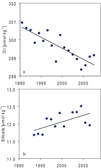
1 1 .0 1 1 .5 1 2 .0 1 2 .5 1 3 .0 1 9 9 0 1 9 9 5 2 0 0 0 2 0 0 5 S ili c a te [µ m o l k g -1 ] bFig. 8. Annual means of (a) dissolved oxygen and (b) silicate over
the years at 2000 m depth at OWSM, with regression lines. Equa-tions, number of data points, R2, and significance level for the two regression lines are for (a) y=–0.12·x+543, 18, 0.71, and 99%; and for (b) y=0.038·x–63.2, 13, 0.36, and 97%.
year. This information eliminates the observed deep water CT increase as a temperature effect, since a similar increase
in CT requires a decrease in temperature.
The general assumption is that the deep basin of the Nor-wegian Sea is fed by a mixture of deep water from the Green-land Sea, which traditionally has been colder and fresher than the deep water of the Norwegian Sea, and Arctic Ocean Deep Water, which has been warmer and saltier compared to the Greenland Sea Deep Water (e.g. Swift and Koltermann, 1988). During the 1980s the deep convection in the Green-land Sea slowed down considerably in the sense that the con-vection was not as deep as it previously was and only reached intermediate depths (Schlosser et al., 1991). This induced a change in the exchange between the deep basins in the
Arc-tic and Nordic Seas, and a larger fraction of old ArcArc-tic Ocean Deep Water would enter the deep Greenland Sea and eventual also the deep Norwegian Sea compared to previously. This was documented by Blindheim and Rey (2004) who showed that the oxygen and silicate concentrations in the deep Green-land Sea decreased and increased, respectively, over the pe-riod from 1980s to 2000. This indicated an increased inflow of old Arctic Ocean Deep Water in which more reminerali-sation of organic matter had occurred. A consequence of this was also that the deep water in the Greenland Sea and Nor-wegian Sea warmed (Blindheim and Rey, 2004; Blindheim and Østerhus, 2005).
Figure 8 shows dissolved oxygen and silicate data from the OWSM deep water, and a similar trend as in the Greenland Sea Deep Water is seen, with the regression lines showing a decrease in oxygen of about 0.12 µmol kg−1yr−1and an increase in silicate of about 0.04 µmol kg−1yr−1. To deter-mine the change in the deep inorganic carbon caused by the changes in water mass composition a Redfield ratio between carbon and oxygen (Rc:o) of 106:–138 is used (Redfield et
al., 1963), and the increase of carbon in the deep water due to decay of organic matter is determined to be about 0.09 µmol kg−1yr−1. This natural process represents about 15% of the observed carbon increase of 0.57 µmol kg−1yr−1.
The anthropogenic part of the observed deep water CT
increase might have several possible sources which will be discussed further. Olsen et al. (2006) estimated an anthro-pogenic increase in CT in the Greenland Sea surface water
ranging between 0.6 and 0.7 µmol kg−1 yr−1. The water convected in the Greenland Sea (down to 1500–1600 m in 2002; Ronski and Bud´eus, 2005) spreads along isopycnals and eventually enters the deep water circulation, a branch of which is the cyclonic circulation in the Norwegian Sea. It is reasonable to assume that this transport route might take about 5 years, assuming a deep current speed of 1 cm s−1, which is a tenth of the velocity reported by Orvik et al. (2001) for deep water at 64◦N 1.5◦E. Along the way from the Greenland Sea to OWSM the water is mixed with surrounding waters and the anthropogenic signal might be diluted, but it is difficult to estimate to which extent.
The observed deep water CT increase at OWSM might
also be explained by turning the view to the Iceland Sea. Blindheim and Rey (2004) suggest that water from the Ice-landic Sea is transported further east to join the cyclonic circulation in the deep Norwegian Sea, and this is based on the observed similar characteristics of bottom waters in the Iceland Sea and the deep Norwegian Sea. According to J´onsson (1992) the strong and positive wind-stress curl dur-ing winter in the centre of the Icelandic gyre might give rea-son to deep convection in this area, and hereby bringing an anthropogenic carbon signal down in the water column. A fraction of this newly formed Iceland Sea Deep Water enters the south-western Norwegian Sea, joins the cyclonic gyre there, and finally reaches the OWSM deep water.
Another source is found by addressing the recirculated Atlantic Water, which has its origin in the northward flow-ing Norwegian Atlantic Current where it receives its anthro-pogenic signal (about 1 µmol kg−1yr−1to the north of the Boreas Basin surface water according to Olsen et al., 2006). It is subducted in the Fram Strait, and a fraction returns southwards into the Nordic Seas as a component of the East Greenland Current (Rudels et al., 1999). Part of this water continues into the Iceland Sea and enters the East Icelandic Current (e.g. Rudels et al., 2002). On its way the recirculated water is modified due to mixing with surrounding waters and part of it might finally enter the south-western Norwegian Sea and join the cyclonic circulation of the Norwegian Sea Deep Water. The time between the sinking of the Atlantic Water and its appearance in OWSM deep water is less than 10 years based on an effective current speed of 1 cm s−1. Therefore, an anthropogenic signal might have been trans-ported towards OWSM via the Iceland Sea, resulting in the observed and estimated annual increase of deep water inor-ganic carbon.
6 Summary
Observations of inorganic carbon, nutrients, and hydrogra-phy at OWSM in the Norwegian Sea show that over years inorganic carbon has increased in the whole water column, and at a higher rate in the surface water compared to the deep water. This increase is verified by an extended multi linear regression method (eMLR). In the surface layer the carbon increase, converted to pCO2, is larger than the observed at-mospheric increase, which is in contradiction to model re-sults.
The observed deep water carbon increase is of both natu-ral and anthropogenic origin and has sevenatu-ral possible expla-nations; (a) remineralisation due to increased fraction of old Arctic Ocean Deep Water; (b) anthropogenic carbon input via the Greenland Sea surface water, the Iceland Sea surface water, and/or transported with the recirculated Atlantic Wa-ter. Remineralisation of organic matter represents about 15% of the deep water carbon increase observed at OWSM, but the contribution from the different pathways of the anthro-pogenic sources are difficult to quantify.
Acknowledgements. Financial support from the Bjerknes Centre
for Climate Research (BCCR) and the Geophysical Institute, University of Bergen, are greatly appreciated. The authors are grateful to the captains and crews of M/S Polarfront who kindly did all the water sampling, and to the shipping company Misje Rederi and the Norwegian Meteorological Institute, which gave us permission to use the ship. F. C. Svendsen kindly provided all the bottle salinity data. We also would like to thank our colleagues for fruitful discussions. This is publication no. A176 from the Bjerknes Centre for Climate Research.
Edited by: J.-P. Gattuso
References
Alvarez, M., Rios, A. F., and Perez, F. F.: Transports and budgets of total inorganic carbon in the subpolar and tem-perate North Atlantic, Global Biogeochem. Cy., 17, 1002, doi:10.1029/2002GB001881, 2003.
Anderson, L. G., Chierici, M., Fogelqvist, E., and Johannessen, T.: Flux of anthropogenic carbon into the deep Greenland Sea, J. Geophys. Res., 105(C6), 14 339–14 345, 2000.
Anderson, L. G. and Olsen, A.: Air-sea flux of anthropogenic car-bon dioxide in the North Atlantic, Geophys. Res. Lett., 29, 1835, doi:10.1029/2002GL014820, 2002.
Blindheim, J. and Rey, F.: Water-mass formation and distribution in the Nordic Seas during the 1990s, ICES J. Mar. Sci., 61, 846– 863, 2004.
Blindheim, J. and Østerhus, S.: The Nordic Seas, Main Oceano-graphic Features, in: The Nordic Seas – An integrated perspec-tive, AGU Geophysical Monograph, 158, dited by: H. Drange, T. Dokken, T. Furevik, R. Gerdes, and W. Berger, 11–37, 2005. Brewer, P. G.: Direct observation of the oceanic CO2increase,
Geo-phys. Res. Lett, 5, 997–1000, 1978.
Brewer, P. G., Glover, D. M., Goyet, C., and Shafer, D. K.: The pH of the North Atlantic Ocean: Improvements to the global model for sound absorption in seawater, J. Geophys. Res., 100, 8761– 8776, 1995.
Chen, C.-T. A. and Millero, F. J.: Gradual increase of oceanic CO2,
Nature, 277, 205–206, 1979.
Chen, C.-T. A., Jones, E. P. and Lin, K.: Wintertime total car-bon dioxide measurements in the Norwegian and Greenland Sea, Deep Sea Res., 37, 1455–1473, 1990.
Dale, T., Rey, F., and Heimdal, B.: Seasonal development of phy-toplankton at a high latitude oceanic site, Sarsia, 84, 419–435, 1999.
DOE: Handbook of methods for the analysis of the various param-eters of the carbon dioxide system in sea water, ver. 2, edited by: A. G. Dickson and C. Goyet, ORNL/CDIAC-74, 1994. Falck, E. and Anderson, L. G.: The dynamics of the carbon cycle in
the surface water of the Norwegian Sea, Mar. Chem., 94, 43–53, 2005.
Friis, K., K¨ortzinger, A., P¨atsch, J., and Wallace, D. W. R.: On the temporal increase of anthropogenic CO2in the subpolar North
Atlantic, Deep-Sea Res. Pt. I, 52, 681–698, 2005.
Gislefoss, J. S., Nydal, R., Slagstad, D., Sonninen, E., and Holm´en, K.: Carbon time series in the Norwegian Sea, Deep-Sea Res. Pt. I, 45, 433–460, 1998.
Goyet, C, Coatanoan, C., Eischeid, G., Amaoka, T., Okuda, K., Healy, R., and Tsunogai, S.: Spatial variation of total CO2and
total alkalinity in the northern Indian Ocean: A novel approach for the quantification of anthropogenic CO2in seawater, J. Mar.
Res., 57, 135–163, 1999.
Gruber, N., Sarmiento, J. L., and Stocker, T. F.: An improved method for detecting anthropogenic CO2in the oceans, Global Biogeochem. Cy., 10, 809–837, 1996.
Johnson, K. M., Wills, K. D., Butler, D. B., Johnson, W. K., and Wong, C. S.: Coulometric total carbon dioxide analysis for ma-rine studies, Mar. Chem., 44, 167–187, 1993.
J´onsson, S.: The sources of fresh water in the Iceland Sea and the mechanisms governing its interannual variability, ICES Marine Science Symposia, 195, 62–67, 1992.
defini-tion for ocean mixed layer depth, J. Geophys. Res., 105, 16 803– 16 821, 2000.
Lewis, E. and Wallace, D. W. R.: Program Developed for CO2 Sys-tem Calculations, ORNL/CDIAC-105, Carbon Dioxide Informa-tion Analysis Center, Oak Ridge NaInforma-tional Laboratory, US De-partment of Energy, Oak Ridge, Tennessee, 1998.
Mosby, H.: Water, salt and heat balance of the North Polar Sea and of the Norwegian Sea, Geophysica Norvegica, 24, 289–313, 1962.
Nilsen, J. E. Ø. and Falck, E.: Variations of Mixed Layer Properties in the Norwegian Sea for the period 1948–1999, Prog. Oceanogr., 70, 58–90, 2006.
Olsen, A., Omar, A. M., Bellerby, R. G. J., Johannessen, T., Ninne-mann, U., Brown, K. R., Olsson, K. A., Olafsson, J., Nondal, G., Kivim¨ae, C., Kringstad, S., Neill, C., and Olafsdottir, S.: Mag-nitude and Origin of the Anthropogenic CO2Increase and13C
Suess Effect in the Nordic Seas Since 1981, Global Biogeochem. Cy., 20, GB3027, doi:10.1029/2005GB002669, 2006.
Omar, A. and Olsen, A.: Reconstructing the time history of the air-sea CO2disequilibrium and its rate of change in eastern subpolar
North Atlantic, 1972–1989, Geophys. Res. Lett., 33, L04602, doi:10.1029/2005GL025425, 2006.
Orvik, K. A., Skagseth, Ø., and Mork, M.: Atlantic Inflow to the Nordic Seas: current structure and volume fluxes from moored current meters, VM-ADCP and SeaSOAR-CTD observations, 1995–99, Deep-Sea Res. Pt. I, 48, 937–957, 2001.
Redfield, A. C., Ketchum, B. H., and Richards, F. A.: The influence of organisms on the composition of seawater, in: The Sea, edited by: M. N. Hill and J. Wiley, New York, 26–77, 1963.
Rey, F.: Phytoplankton: The grass of the sea, in: The Norwegian Sea Ecosystem, ed. H.R. Skjoldal, Tapir, Trondheim, Norway, 93–132, 2004.
Ronski, S. and Bud´eus, G.: Time series of winter convec-tion in the Greenland Sea, J. Geophys. Res., 110, C04015, doi:10.1029/2004JC002318, 2005.
Rudels, B., Friederich, H. J., and Quadfasel, D.: The Arctic circum-polar boundary current, Deep-Sea Res. Pt. II, 46, 1023–1062, 1999.
Rudels, B., Fahrbach, E., Meincke, J., Bud´eus, G., and Eriksson, P.: The East Greenland Current and its contribution to the Denmark Strait overflow, ICES J. Mar. Sci., 59, 1133–1154, 2002. Sabine, C. L., Key, R. M., Johnson, K. M., Millero, F. J.,
Pois-son, A., Sarmiento, J. L., Wallace, D. W. R., and Winn, C. D.: Anthropogenic CO2inventory of the Indian Ocean, Global Bio-geochem. Cy., 13, 179–198, 1999.
Schlosser, P., B¨onisch, G., Rhein, M., and Bayer, R.: Reduction of Deepwater Formation in the Greenland Sea During the 1980s: Evidence from Tracer Data, Science, 251, 1054–1056, 1991.
Skjelvan, I., Olsen, A., Anderson, L. G., Bellerby, R. G. J., Falck, E., Kasajima, Y., Kivim¨ae, C., Omar, A., Rey, F., Olsson, K. A., Johannessen, T., and Heinze, C.: A Review of the Inorganic Carbon Cycle of the Nordic Seas and Barents Sea, in: The Nordic Seas – An integrated perspective, AGU Geophysical Monograph, 158, edited by: H. Drange, T. Dokken, T. Furevik, R. Gerdes, and W. Berger, 157–175, 2005.
Solomon, S., Qin, D., Manning, M., Alley, R. B., Berntsen, T., Bindoff, N. L., Chen, Z., Chidthaisong, A., Gregory, J. M., Hegerl, G. C., Heimann, M., Hewitson, B., Hoskins, B. J., Joos, F., Jouzel, J., Kattsov, V., Lohmann, U., Matsuno, T., Molina, M., Nicholls, N., Overpeck, J., Raga, G., Ramaswamy, V., Ren, J., Rusticucci, M. Somerville, R., Stocker, T. F., Whetton, P., Wood R. A., and Wratt, D.: Technical Summary, in: Climate Change 2007: The Physical Science Basis, Contribution of Working Group I to the Fourth Assessment Report of the Intergovernmen-tal Panel on Climate Change, edited by: Solomon, S., Qin, D., Manning, M., Chen, Z., Marquis, M., Averyt, K. B., Tignor M., and Miller, H. L., Cambridge University Press, Cambridge, UK and New York, NY, USA, 2007.
Swift, J. H. and Koltermann, K. P.: The origin of Norwegian Sea deep-waters, J. Geophys. Res., 93, 3563–3569, 1988.
Takahashi, T., Sutherland, S. C., Sweeney, C., Poisson, A., Metzl, N., Tilbrook, B., Bates, N., Wanninkhof, R., Feely, R. A., Sabine, C., Olafsson, J., and Nojiri, Y.: Global sea-air CO2flux based on
climatological surface ocean pCO2, and seasonal biological and temperature effects, Deep-Sea Res. Pt. II, 49, 1601–1622, 2002. Tanhua, T. and Wallace, D. W. R.: Consistency of TTO-NAS in-organic carbon data with modern measurements, Geophys. Res. Lett., 32, L14618, doi:10.1029/2005GL023248, 2005.
Tans, P. P. and Conway, T. J.: Monthly Atmospheric CO2
Mix-ing Ratios from the NOAA CMDL Carbon Cycle Cooperative Global Air Sampling Network, 1968-2002, in: Trends: A Com-pendium of Data on Global Change, Carbon Dioxide Informa-tion Analysis Center, Oak Ridge NaInforma-tional Laboratory, US De-partment of Energy, Oak Ridge, Tenn., U.S.A, 2005.
Wallace, D. W. R.: Monitoring global ocean carbon inventories, OOSDP Background Report No. 5, Texas A&M University, Col-lege Station, Texas, USA, pp. 54, 1995.
Wallace, D. W. R.: Storage and transport of excess CO2 in the
oceans: The JGOFS/WOCE global CO2Survey, in: Ocean
cir-culation and climate: observing and modelling the global ocean, edited by: G. Siedler, J. Church, and J. Gould, 489–521, 2001. Østerhus, S. and Gammelsrød, T.: The abyss of the Nordic Seas is
![Fig. 2. Hovm¨oller diagram of water column (a) temperature [ ◦ C] and mixed layer depth (white line), (b) salinity, (c) C T [µmol kg −1 ], (d) nitrate [µmol kg −1 ], and (e) silicate [µmol kg −1 ] during the period 2001 throughout 2006.](https://thumb-eu.123doks.com/thumbv2/123doknet/14795495.603592/4.892.170.726.136.971/hovm-diagram-column-temperature-salinity-nitrate-silicate-period.webp)