Effective elastic thickness and crustal thickness variations in west central Africa inferred from gravity data

HAL Id: insu-01356057

https://hal-insu.archives-ouvertes.fr/insu-01356057

Submitted on 24 Aug 2016

HAL is a multi-disciplinary open access

archive for the deposit and dissemination of

sci-entific research documents, whether they are

pub-lished or not. The documents may come from

teaching and research institutions in France or

abroad, or from public or private research centers.

L’archive ouverte pluridisciplinaire HAL, est

destinée au dépôt et à la diffusion de documents

scientifiques de niveau recherche, publiés ou non,

émanant des établissements d’enseignement et de

recherche français ou étrangers, des laboratoires

publics ou privés.

Effective elastic thickness and crustal thickness

variations in west central Africa inferred from gravity

data

Y. Poudjodmj Oma, J. Nnange, M Diament, C.J. Ebinger, J Fairhead

To cite this version:

Y. Poudjodmj Oma, J. Nnange, M Diament, C.J. Ebinger, J Fairhead. Effective elastic thickness

and crustal thickness variations in west central Africa inferred from gravity data. Journal of

Geo-physical Research : Solid Earth, American GeoGeo-physical Union, 1995, vol.100 (B11), pp.22047-22070.

�10.1029/95JB01149�. �insu-01356057�

JOURNAL OF GEOPHYSICAL RESEARCH, VOL. 100, NO. B 1 l, PAGES 22,047-22,070, NOVEMBER 10, 1995

Effective

elastic thickness and crustal thickness variations

in west central Africa inferred from gravity data

Y. H. Poudjom

Djomani,

1'2

J. M. Nnang½,

2'3

M. Diamcnt,

and J. D. Fairhead

2

1 C. J. Ebinger,

2

Abstract. The west central African region is characterized by various geological features: Cretaceous rifts (Benue), Tertiary domal uplift (Adamawa volcanic uplift), Tertiary-Recent volcanoes (Cameroon Volcanic Line or CVL), Tertiary sedimentary basins (Chad basins), and cratonic region (Congolese craton). In this study, we investigate the relationship between these tectonic features and the flexural rigidity of the lithosphere in Cameroon, in terms of effective elastic thickness (Te), by the use of the coherence function analysis. For that purpose, we use a new dataset of-32,000 gravity and topography points from Cameroon and the adjacent countries. The Te contour map deduced from this study shows a good relationship between the tectonic provinces and the rigidity of the lithosphere, the minima (14-20 km) are beneath the active rifted and volcanic areas (Benue, CVL, and Adamawa), and the maxima (-40 km) correspond to the Archean reworked unit in Congo. A spectral analysis of the gravity data is performed to determine the crust-mantle boundary in these tectonic provinces. The crustal thickness (Tc) contour map shows a variation from 14 km to about 45 km, consistent with other geophysical data. The lower values (14-20 km) are obtained in central Cameroon on the Adamawa uplift, and the highest values are found in southern Cameroon (Archean reworked Congolese craton). Comparing Te and Tc values shows that there is generally a positive correlation between the two parameters, with an exception in Chad where this correlation is rather negative.

Introduction

Research into the origin of large igneous provinces (LIPs) worldwide has led some scientists to propose that lithospheric structural discontinuities in part control the location of oceanic plateaus and continental flood basalt provinces [e.g., Hopper et al., 1992; Anderson, 1994]. One of these LIPs, the Cameroon Volcanic Line (CVL) extends across both oceanic and continental lithosphere, but volcanism shows no age progression [e.g., Fitton and Dunlop, 1985]. The continental part of the CVL and surrounding regions can be divided into

two domains: a mobile belt in the north and a cratonic belt in

the south, with the seismically and volcanically active CVL lying between the two (Figure 1).

The flexural rigidity (D), or equivalently, the effective elastic thickness (EET or Te), describes the manner in which a plate responds to lateral density variations applied at the surface or within the plate. Studies of T e and its variations within the oceanic plates show that T e is dependent upon the thermal structure of the plate, and studies of the more complicated continental plates also show some thermal dependence, although the temperature is not the only factor that controls T e in continents [e.g., Burov and Diament, 1995]. Thus lateral variations in T e may provide information on the location and depth extent of thermal and structural

t Laboratoire de Gravim6trie et G60dynamique, Institut de Physique

du Globe, Paris.

2Department

of Earth

Sciences,

University

of Leeds,

Leeds,

England.

Paper number 95JB01149. 0148-0227/95/95JB-01149505.00

discontinuities within the lithosphere. The objective of our study is to investigate variations in lithospheric structure beneath west central Africa, including the continental region of the CVL, and to relate these variations to Cenozoic rifting and volcanic processes.

Gravity and topography data from continental regions provide a means of mapping out variations in crustal thickness and mechanical thickness of the lithosphere. Forsyth [1985] introduced the coherence function as a robust means of estimating T e in continental regions. Unlike

admittance functions, the coherence method assumes that

topographic relief reflects both surface and subsurface density contrasts, or loads, and exploits the relationship between the Bouguer gravity and topography as a function of the wavelength. In this study, we first estimate the thickness of the crust (T c) throughout west central Africa by means of the gravity power spectra [e.g., Spector and Grant, 1970]. We then use the coherence method to examine variations in T e throughout the study region, using existing seismic data to constrain density models.

Geological Setting

The area of investigation (Figure 1) is a part of the central African mobile belt and also includes a part of the Congolese craton. The latter was created during the Liberian cycle (2800 Ma) and rejuvenated during the Ebumean (230 -1800 Ma). The entire area was affected by the Pan-African cycle (600 + 100 Ma) during which important tectonic movements occurred, giving rise to megashear zones in Africa [e.g., Ngako et al.,

1991]. One of these zones, oriented ENE-WSW, is called the Central African Shear Zone (CASZ) and extends over about 2000 km from Sudan to Cameroon [Cornacchia and Dars, 1983; Moreau et al., 1987; Ngako et al., 1991]. It is a dextral

22,048 POUDJOM DJOMANI ET AL.: ELASTIC THICKNESS IN WEST AFRICA PLATEAU 10øN 5øN • "•' BIU ß PLATEAI ADA Foumban , m Yaounde

'

CASZ : Central African Shear Zone FSZ:FoumbanShearZone

Sedimentary cover Basement Igneous rocks

/

Tertiary-Quaternary

•

Proterozoic

ii• Volcanics

•

Mesozoic

•

Panafrican

•

Younger

granites

•

Northern

margin

of

Fault

Shear

Zone t'' the

congolese

craton

Figure 1. Geological map of the study area. The northern limit of the Congolese craton is not well known to the east of the area. Volcanic centers between Mount Oku and Biu plateau are not shown. Also shown are the Precambrian and reworked faults (e.g., CASZ, Sanaga). After Cornacchia and Dars [1983] and Sanaga fault zone from Dumont [ 1986].

shear zone associated with broad mylonite belts predating the opening of the South Atlantic Ocean in Cretaceous times [e.g., Jorgensen and Bosworth, 1989]. This fault extends into Brazil as the Pernambuco polycyclic lineaments [De Almeida and Black, 1967; Martin et al., 1981; Popoff, 1988]. Parallel to this fault zone and to the south of it is the Sanaga fault zone. It is also a dextral shear running from Cameroon to Central African Republic [Dumont, 1986].

The "younger granites" of the Jos plateau in Nigeria, roughly oriented along a N-S axis, give Rb-Sr ages between 213 and 141 Ma [Rahaman et al., 1984; Vail, 1989]. Their origin is related either to the migration of the African plate over a mantle plume [e.g., Karche and Vachette, 1976] or shear movements along preexisting ENE-WSW trending faults in the Pan-African basement [e.g., Black et al., 1985].

The opening of the South Atlantic Ocean in Cretaceous times resulted in a series of basins and grabens in the study

area,

such

as the Benue

in Nigeria-Cameroon,

the Mb•re and

POUDJOM DJOMANI El' AL.: ELASTIC'THICKNESS IN WEST AFRICA 22,049 6 8 10 12 14 16 18 20 1 14 12 10 CHAD 6 8 10 12 14 16 18 20 12 10 metres Above 2000 1800 - 2000 1600 - 1800 1400 - 1600 1200 - 1400 1000 - 1200 800 - 1000 600 - 800 400 - 600 200 - 400 0- 200 Below 0 • Undef

East longitudes

Plate 1. Topographic map of west central Africa. Note the high altitudes over the Jos, Biu and Adamawa plateaus and the volcanic centers of the Cameroon Volcanic Line oriented in a N70 ø to 90 ø direction (refer to Figure 1 for location of these features). The Benue trough and the Chad sedimentary basins are characterized by altitudes less than 400 m. CAR, Central African Republic.

6 8 10 12 14 16 18 20 , 14 8 10 i ' -- i ! i .... 12 14 16 18 20 -12 '10 mGal Above 20 10 - 20 0- 10 '.T77 40- o -_:2] -•o- 40 ___-•_• -30 - -20 -40 - -30 • -50 - -40 -60 - -50 • -70 - -60 -80 - -70 -90 - -80 -100 - -90 I Below -100 :_-_•21 un,•,• East longitudes

Plate 2. Bouguer anomaly map of Cameroon and the adjacent countries computed using the data in Figure 2. The map is dominated by a long-wavelength negative Bouguer anomaly in central Cameroon corresponding to the Adamawa uplift, negative anomalies on the Congolese craton, and positive anomalies on the Benue trough (refer to Figure 1 for the location of these features).

22,050 POUDJOM DJOMANI E-'I' AL.: ELASTIC THICKNESS IN WEST AFRICA

trough is characterized by a broad positive Bouguer anomaly interpreted as crust that has been thinned and replaced by anomalous upper mantle material [e.g., Fairhead and Okereke, 1987]. The Mbere and Djerem sedimentary basins are limited to the north by the CASZ (known in Cameroon as the Foumban shear zone, or Ngaoundere rift) and characterized by conglomerates and mylonites localized along the fault zone [Ngangom, 1983]. The Chad basin is one of the African

intracontinental basins in the Pan-African reactivated

basement. Its origin is controversial: Burke [1976], and, recently, Genik [1992] suggest that the basin owes its origin to the existence of a number of peripheral uplifts and is underlain by deep rift systems formed in Early Cretaceous during the separation of Africa from South America. Cratchley et al. [1984] and Freeth [1984] suggest a Precambrian origin

for the basin.

The area is also dominated by a series of Tertiary-Recent volcanic centers that form the CVL. This 1600-km-long line straddles the west African continental margin, and extends from the Atlantic Ocean to the Biu plateau in northern Nigeria

(Figure 1). Magmatic activity has occurred on the line from 65 Ma to Present and shows no age progression [Fitton and Dunlop, 1985]. A part of the line runs eastward toward the Adamawa volcanic uplift in central Cameroon (Figure 1). Thus the line seems to be superimposed on the preexisting CASZ which cuts across the Adamawa uplift [e.g., Moreau et al., 1987' De'ruelle et al., 1991; Wilson and Guiraud, 1992]. Seismological studies revealed low upper mantle velocities, interpreted as an abnormally hot upper mantle beneath the Adamawa uplift, and a lithospheric thinning [Dorbath et al., 1986; Plomerova et al., 1993]. Several earthquakes have been registered in the area within the last 5 years, with magnitudes up to 4.8. Seismological studies show that this recent seismic activity is related to the magmatic activity of the line [Tabod

et al., 1992].

The topographic map of the study area correlates well with the tectonic provinces (Plate 1). The 130-km-wide Jos plateau is characterized by elevations above 800 m. Also elevated is the 700-m-high Biu plateau. The highest elevations occur in southwest Cameroon and correspond to the volcanic centers of

6 8 E E E 1 E E E 13N 11N 9N 7N SN ß +

'.'...

NIGERIA

A'Llan'Lic

Ocean

o

EG

lIBON

ZAIRE

Figure 2. Gravity data distribution in Cameroon and adjacent countries. EG, Equatorial Guinea. See text for

POUDJOM DJOMANI E1 AL.: ELASTIC THICKNESS IN • AFRICA 22,051

Political boundary

Figure 3. The 33 grids used for the estimation of T e, as well as for the Moho depth. Note that the grids are overlapping on each other. All the grids are numbered in their center.

the CVL. In this area, Mount Cameroon, the only active

volcano of the line, rises to 4095 m. The Cretaceous Benue

trough is characterized by altitudes less than 200 m, and steep topographic gradients on the flanks, whereas the Tertiary sedimentary basins in Chad are at altitudes between 300 m and 500 m. The Congolese craton is characterized by altitudes between 500 m and 800 m. The study area thu. s encompasses several geological features, of different ages, length scales, and elevations, suggesting different modes of isostatic compensation and/or lithospheric structure.

Data and Grids

The data used in this study were acquired during several surveys carded out in Cameroon and adjacent countries by (1) ORSTOM (Institut Franqais de la Recherche Scientifique pour le DEveloppement en CoopEration, France) between 1960 and 1967, (2) J. D. Fairhead in 1982, (3) Nnange [1991] at IRGM (Institute of Geological and Mining Research, Cameroon) and University of Leeds (England), (4) DMA (U.S. Defense Mapping Agency), and (5) ELF Aquitaine oil company (unpublished). These data sets consist of approximately 32,000 irregularly spaced elevation points and corresponding gravitational acceleration values determined from both land and air surveys (Figure 2). Where height information was available, Hammer's [1939] method was used for terrain corrections on the data [Nnange, 1991]. All the data were tied to the IGSN71 reference system. A density reduction of 2670

kg/m

3 was

used

for the Bouguer

correction.

Latitudes

and

ele•nent algorithm [Inoue, 1986; El Abbass et al., 1990]. The total grid has 85 x 79 points (in the x and y directions, respectively), which means 1554 km x 1443 km. The same transformations were applied to the gravity and topographic data. From the total grid, we extracted 33 subgrids of gravity and corresponding topography, each 444 km x 444 km (25 x 25 points). These subgrids (Figure 3) were used to perform source depth estimations by spectral analysis of the gravity data and also to estimate the effective elastic thickness (Te) of the lithosphere.

We computed the two-dimensional (2-D) Fourier transform of the data on each subgrid using the algorithm of Singleton [1969]. This allowed us to obtain the spectral amplitudes of Bouguer gravity and topography. Prior to this transformation, the gridded data were mirrored about their eastern and southern boundaries in order to avoid edge effects. This produced data sets twice the original length and width. The longest wavelengths in the Fourier transform exceed the initial dimensions of the grids, due to mirroring, and were rejected before the inversion for T e.

Plate 2 is a new Bouguer anomaly map of Cameroon and adjacent countries. This map clearly shows the long wavelength negative Bouguer anomaly of about -120 mGal

centered on the Adamawa massif in central Cameroon. This

anomaly is oriented NE-SW near the coast following the

volcanic massifs of the CVL, and it becomes E-W in the

Adamawa region. The long-wavelength negative Bouguer anomaly beneath the Adamawa uplift can be compared to the anomalies of other African uplifts (Hoggar, Air, Darfur, and Tibesti and the Keny a dome) and is commonly interpreted as due to a low-density body in the upper mantle [Browne and Fairhead, 1983; Okereke, 1988].

Located at the western margin of the CVL, the Benue trough is characterized by NE-SW relative positive anomalies of amplitude 40 mGal. These anomalies could be compared to

those of other active rift zones in east Africa. The anomalies

northwestward of the trough are to be interpreted with care because of a lack of data in this area. The SW-NE positive

anomalies observed in Chad correlate with either the

sedimentary basins and grabens that initiated duri. ng Cretaceous times [Genik, 1992] or a basic intrusion into the basement beneath shallow sedimentary cover, which could represent a suture zone [e.g., Freeth, 1984]. We can also note the negative anomalies of the CASZ in central Africa, in a

ENE-WSW trend.

Southern Cameroon is characterized by negative anomalies (-80 mGal) which correspond to the northern part of the Congolese craton. The limit of this craton is marked by a low and regular vertical gradient of about 1 mGa!/km, which marks a change in density of crustal rocks from the north to the south [Collignon, 19•68]. On the gravity map, it is shown as E-W positive anomalies between the negative anomalies to the north (Adamawa uplift) and to the south (Congolese craton). In the next sections, we use these gravity anomalies to constrain the crustal structure and the mechanical lithospheric thickness beneath the CVL and west central Africa to investigate the possible control of the lithosphere on the location of the

CVL.

Structure of the Crust

In this part of the study, we use the 33 subt,_•_ds of Figure 3 to estimate the crustal thickness (Tc) and its variations within

22,052 POUDJOM DJOMANI ET AL.: ELASTIC THICKNESS IN WEST AFRICA

the study area, by spectral analysis of the gravity data. The same subgrids for T e estimations will be used in the second section of the paper.

Method

Spector and Grant [1970] described a statistical method to determine average depths of various magnetic layers by considering the random distribution of sources. This is achieved by a plot of the logarithm of the power of the magnetic anomalies versus the wavenumber. This method was improved and adapted for gravity data by Syberg [1972].

Given a grid of data and its corresponding 2-D Fourier transform, the 2-D power spectrum is calculated by the relation

=

+ xix,y)

where

XR(kx,

ky

) and

Xl(kx,

ky) are the real and

imaginary

_,

_,

_x,

_{ky. After}

spectrum

in concentric

rings

of constant

Ikl,

where

Ikl--(kx2+

ky2)l/2=

2•/•,

and

)• is the

wavelength.

So,

if k denotes

the

wavenumber and S(k) denotes the power spectrum, the depth to the body (h) can be estimated by

h =- Ln [S(k)l/21kl

If we plot the logarithm of the power spectrum versus the wavenumber, some straight-line segments can be identified, the slopes of which are proportional to the depth to the top of the buried body [e.g., Pal et al., 1979; Chakraborty and Argawal, 1992; Poudjom Djomani et al., 1992]. This depth is estimated by a least squares fitting of the linear segments on the data points.

Error Estimations on T c

While computing the power or radial spectrum for source depth estimations, errors due to three important points must be considered: the window size, the data spacing, and the selection of the linear segments on the plots [Dimitriadis et al., 1987]. Regan and Hinze [1976] show that for gravity fields, a window size of 6 times the source depth is required for less than 10% information loss. In our case, each grid is 444 km x 444 km, and we limit depth estimates to 74 km. Grid spacing also affects the depth estimation. According to Cianciara and Marcak [1976], the shallowest depth estimate from a power spectrum must be at least 40% of the grid spacing interval. Since our grid spacing is approximately 18.5 km, this equates to shallowest estimated depth of 7.4 km. The third source of error relates to the choice of the regression lines. In general, more than one linear segment can be seen on the plots; the high frequency components indicate noise effects, the low frequencies indicate the regional effects, and the intermediate frequencies represent the target sources. In this study, we present and discuss only the results corresponding to the depth to the crust-mantle boundary. In order to choose the proper wave band for this depth, we use seismic refraction constraints. That is, on the spectrum corresponding to the only region where some seismic

refraction results are available (in the Adamawa region), first, we define several possible linear segments and estimate the corresponding depths (Figure 4, grid 21). Then we select the wavenumber band that gives a depth closest to the Moho determined from seismic data, i.e., 23 km [Smart et al., 1985].

This

wave

band

is between

0.06 km

-1 and

0.12

km

-1 (Figure

4).

T c Map and Interpretation

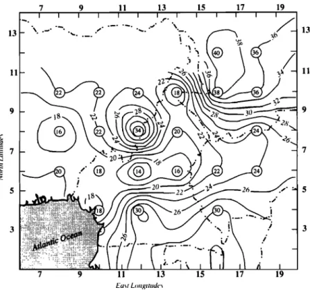
The values of Table 1 were interpolated to compute a map of T c variation within the area (Figure 6). T c varies from 14 km in the NE of the map to 45 km in the south. Also evident on the map is a thinning of the crust along an E-W trend in central Cameroon, beneath the Adamawa uplift. Some clear

trends are visible if we subdivide the area into four blocks: the northeastern, central, transition, and southern blocks.

Northeastern block (grids 5 and 6). This block correlates with the poorly understood region in Chad where little subsurface information exists (Figure 1). The regression line is well defined on both plots, and the corresponding depths (13.6 + 2 km and 14.6 + 1 km for grids 5 and 6, respectively) are the lowest values obtained in the study area. The Chad region has good data coverage, and the size of the box was shown, in the previous section, to be sufficient for the estimation of depths up to 74 km. However, we enlarged the box to 555 km x 666 km and obtained a depth of about 15

km. So, our result here is well constrained. The thickness of a

normal cratonic crust is commonly more than 30 km [e.g., Mourgues, 1983; Sollet et al., 1982; Hadiouche and Jobeft,

1988]. Thus it seems that in this area, the crust-mantle

boundary is masked by a more pronounced intracrustal density

contrast which is determined here. This area needs to be

investigated by additional geophysical methods to confirm

our results.

Central block (grids 15 to 24). This region corresponds to the Adamawa uplift in central Cameroon. The average crustal thickness determined here is between 18 and 23 km. In order to test the reliability of our result in this area, we selected a larger box, 444 km x 888 kin. The slope of the regression line in the selected wave band gives an estimate of 23 + 2 km for the average crustal thickness. These results

show that the crust is thinned in this area relative to the

surrounding, in agreement with seismic refraction studies which show that T c varies from 23 km in the north of the Adamawa uplift to 33 km in the south [Stuart et al., 1985]. On the other hand, petrologic studies carried out on mantle xenoliths suggest that the crust-mantle boundary beneath the Adamawa uplift is not deeper than 25 km [Girod et al., 1984]. The main result here is that the central block (Adamawa uplift) is characterized by a thinning of the crust.

Transition block (grids 7, 8, 9, 10, 11, 13, 14, and 19). This corresponds to all the areas where the crustal

POUDJOM DJOMANI El AL.: ELASTIC THICKNESS IN WEST AbiCA 22,053

Grid 16

Grid 21

7-10:23.4

km

7-12:17.5

lcm

8-14:15.7

lcm

-8

[ '

Grid 22

4 I

-6 1

Figure 4. Selection of the wave bands for the estimation of the average crust-mantle boundary and error estimations: example of grids 16, 21, and 22 corresponding to the Adamawa uplift. For each plot, the first set of points selected give the average crust-mantle boundary. The other sets of points are selected to show the possible variation of the limits of the wavenumber band and the corresponding errors on the depth.

thickness varies from 24 to 33 km. These areas are localized

to the north, the southeast, and south of the Adamawa uplift. To the northwest, the Jurassic Jos granitic plateau in Nigeria is characterized by a 27 + 5 km thick crust. Southward, in the Benue rift, the average crustal thickness is between 15 and 33 km. The 15-km-thick crust belongs to the central lower

Benue, while the 33 km thickness is for the western lower

Benue. A value similar to the latter is found along the northwestern margin of the Adamawa uplift and corresponds to the Gongola rift (a branch of the Benue trough). Previous

gravity studies of the Benue trough show that the amount of crustal extension is about 90 km perpendicular to the axis of the trough [Fairhead and Okereke, 1987, 1990]. Eastward, beneath the Yola rift, T c is about 25 km. These results suggest

that the crust is thinned beneath the Yola rift, north of the

Adamawa uplift. Fairhead and Okereke [1987] performed a three-dimensional inversion of gravity data, taking into account the seismological constraints [Stuart et al., 1985]. This inversion reveals that the average crustal thickness is 20, 23 and 30 km for the lower Benue, the Yola, and the Gongola

22,054 POUDJOM DJOMANI E1 AL.: ELASTIC THICKNESS IN WEST AFRICA Gridl Grid2 O- 0 Tc = 17.8_+1 km

-4-

•

-bø.•O

o.os o.,o o.,s o.•o o.•

-2-

-4-

-6-

Tc = 30.2-t-1 km

oo

-b•.6o

'o.05 'o. io 'o.

i5 'o.•o 'oi•5

E o J Grid3 -2 Tc = 16.2+1 km

-6- "• øo

•.•o -o.05

•o.

i o -o.

i s" o.•o

Grid5 Tc = 15.6.•2 km O- o o c -4 o o o --6! . ,

o.oo o.o5 o. io o. i5 o.•o 0.25

Grid4 -2- -4-

•60 '

0.'65 'o.•o 'o. i5 'o.•o 'o.•s

Grid6 co Tc = 14.6;I;1 km o o o -4- '• C O

•?•o o.os o. io o.,5 o.•o o.•5

Grid7 Grid8 2 Tc = 25.7+4 km 0 o o o c c

•.00 0.05 0.10 0.15 0.20 0.25

-bO.;o

.

.

Wovenumber (1/kin)

Figure 5. Plots of the logarithm of the gravity power spectrum versus the wavenumber, for the 33 grids. For

each

grid the slope

of the selected

regression

line gives

the value

of T c which

is indicated

at the upper

right

POUDJOM DJOMANI E1 AL.: ELASTIC THICKNESS IN WEST AFRICA 22,055 Grid9 Grid10

O-C• 1½

= •.6::1:.8

km

-•

<o o o

-•6.•0 0.05 0.10 0.15 0.20

Oo

ø Tc = 24.4.•5

km

>'

-•760 o.0s o,o o.,• o.•o o.•

> cn Grid13 a'• 4 o _..I 2 Tc = 33.7.-1:6 km o

•)8.•0 0.05 0.10 0.15 0.20 0.25

•.oo-o.os o.•o o.•s o.•o o.•s

Grid14 Tc = 14.9.-!:.1 km 0

08.00

0.05 0.10 0.15 0.20 0.25

Wovenumber (1/l•m •

22,056 ,POUDJOM DJOMANI ET AL.: ELASTIC THICKNESS IN WEKr AFI•CA Grid17 Grid18 Tc = 11.4-t-1 km o 0 oo o

-2- •o

•6o o.0• 'o.

io 'o.i• 'o.•o

•0.•

O- -4- oo Tc = 16.7-1-4 km o o o o o o

'38.00

'o.05 o.•o o. i5 'o.:•o

'0.2.-

Grid19 4

:3 i

Tc

= 31.7:1:8

km

->' 'b"!o

o.o•

o.

io o.• 0.20

-o.•

c• Grid21 • 4 0 o Tc = 22.5+4 km o 0 oo -4

6

o o

08.00

o.o• o.

io o.i• o.•o o.:•

Grid20

o

2 0 Tc = 22.6+3 km

o c•

-2 oo

-•86o

•0.0• 'o.,o o.,• o.•o 'o.•

Grid22

-2

Tc = 20.5+3 km

Oo

•.•o o.o• o.•o o.•s o.•o o.a•

Grid23 Grid24 o 2 Tc = 21.2.•8 km 0 oO o o 6 c o 0.00 0.05 0.10 0.15 0.20 0.25 -2 -4 O 2 Tc = 22+7 km c 0 0 o o -2 o

o•.•o

.

.

Wovenumber

.POUDJOM

DJOMANI

EI AL.:

ELASTIC

THI•SS IN WEST

AFRICA

-b?(•o

o.b• 'o. io '

o o o. i5 o.•o o.•5 2. 00 Tc = 29.7ñ1 km O- o _•. o --4' o o

ß o 'o.65 'o. io 'o.i5 'o.•o 'o.•. •

22,057 Grid27 E tO 0- Q. • -2- Tc = 524-4 km o o o o o •. 8 • -• o.oo 0.05 O. lO 0. iS 0.20 0.25 ,.... c• Grid29 [j• 2 o o -2 c O, Tc = 59:1=3 km 4 o o

6

• o o o

•o o.o• o. io o.• o.zo o.z•

41

2t

o0 Tc

= 40.-1:5

km

ø1%

-4

0

•)8.•o

0.05 o.•o 0.•5 o.•o

Grid30 o Tc = 47+10 km 2 o o 0 -2 0.00 0.05 0.10 0.15 0.20 0.25 Grid31 -2 -4 -6 c o o Tc = 45;I;8 km o c C ..8 I 0.00 0.05 0.10 0.15 0.20 0.25 Grid32 Tc = 5i+10 km -2 6 ,'3. 8

o.oo 0.05 o.•o o.• o.•o ø.z5

Wavenumber (1/km)

22,058 POUDJOM DJOMANI ET AL.: ELASTIC'THICKNESS IN WEST AFRICA

Grid33

Tc -

45.8ñ5

km

0.65 o. io 'o.i5 'o.o 'o.z5

Wvenumber (1/kin)

Figure 5. (continued)

riffs, respectively. According to these estimates and in the

view of our results, the crust is thinner in the lower than in the

upper Benue rift.

To the south of the Adamawa uplift, T c increases to 26 km. This value is consistent with seismic data which suggest that

the crust becomes thicker as one moves southwards of the

uplift [Stuart et al., 1985]. This area appears to be a transition

zone between the "Pan African" and the "cratonic" crust here

after presented.

Southern block (grids 25 to 33). T c estimates are more than 30 km and could be as high as 50+ 10 km in the northern part of the Congolese craton. A larger grid (333 km x 666 km) produces a T c of about 29 km, which is less than the previous 50 km. This could be due to the data distribution, since the larger grid also includes some areas with very few data. The results show that in the Congolese craton area the

crust is thicker than beneath the mobile belts and rifted

regions to the north.

Mechanical Behavior of the Lithosphere

Observed coherence

The method used to estimate the flexural rigidity (D), or, equivalently the effective elastic thickness (Te)of the lithosphere, is the coherence function analysis [e.g., Forsyth, 1985]. This method exploits the wavelength dependence between gravity and topography. Flexural models of isostatic compensation for continental lithosphere assume that a thin elastic plate overlying a fluid asthenosphere is deflected by surface (e.g., topographic) and subsurface (e.g., Moho) loads. The amplitude and wavelength of the deflection of the plate thus depend on the flexural rigidity and distribution of the loads. For example, the classical Airy model (local compensation) corresponds to a flexural model where the plate has no rigidity. If the plate has a nonzero rigidity (regional compensation), at short wavelengths, surface and subsurface loads are supported by the rigidity of the lithosphere and the plate is not deflected. As a consequence, the gravity and

topography are incoherent and the coherence is close to 0. At long wavelengths, the plate is deflected by surface loads, and loading from below leads to the formation of topographic reliefs. Therefore gravity and topography are coherent and the coherence is close to 1. The steep curves at the transitional wavelength where loads are partially supported by plate strength and by flexure give an estimate of the flexural rigidity of the lithosphere (Figure 7). The T e and the flexural rigidity of a plate are related by

D = ETe

3 / [12(1-

v2)],

(1)

The observed coherence is computed, in the frequency domain, by [Forsyth, 1985]:

yo2(k)

= Cs

2 (k) / [EH(k)

EG(k)I

(2)

where

Cs

2 (k) is the

square

of the

cross

spectrum

of gravity

and

topography,

EH(k)

= <H(k)

H*(k)>

is the

average

spectrum

of

topography,

EG(k

) = <G(k)G*(k)>

the

average

spectrum

of

gravity, asterisk is the complex conjugation, and k=lkl the

two-dimensional

wavenumber

is

equal

to

(kx

2 + ky2)

1/2,

k

x and

ky are wavenumbers

in the

x and

y directions,

respectively.

In

1966]

T

2 = (nTo

2 - 1)/(n-

1)

(3)

Grid Selected Wavebands 'rc, km 1 7to 12 17.8_+ 1 2 7 to 10 30.2 _+ 1 3 9 to 13 16.2 _+ 1 4 8to 11 20.7 _+4 5 8to 14 13.6_+2 6 8to 13 14.6_+ 1 7 8 to 11 25.7 + 4 8 8to 11 28.8+6 9 6 to 9 33.6 _+ 8 10 6 to 10 28.0 _+ 5 11 6 to 10 24.4 _+ 3 12 8 to 11 25.7 _+ 1 13 6 to 10 33.7 _+ 6 14 9 to 15 14.9 _+ 1 15 9 to 13 18.5 _+ 2 16 7 to 10 23.4 _+ 6 17 9 to 14 11.4 _+ 1 18 5to8 16.7 _+ 4 19 6 to 9 31.7 _+ 8 20 6 to 10 22.6 _+ 3 21 9 to 12 22.5 + 4 22 10 to 12 20.5 + 3 23 8 to 11 21.2 _+ 8 24 8 to 11 22.0 _+ 7 25 8 to 10 35.0 _+ 10 26 6 to 10 29.7 _+ 1 27 4 to 8 32.0 _+ 4 28 7 to 10 40.0 _+ 5 29 4 to 8 59.0 _+ 3 30 8 to 10 47.0 _+ 10 31 6 to 9 45.0 _+ 8 32 6 to 10 51.0 + 10 33 5 to 10 45.8 -+ 5

POUDJOM

DJOMANI

E1 AL.: ELASTIC

THICKNESS

IN WEST

AFRICA

22,059

3o•

x

/

22

/ ?'"

'•"

%

2

2

•

W•

, ;••••._••

Figure

6. Average

crustal

thickness

contour

map

of the

study

area

obtained

by interpolation

of the

values

in

Table 1. Contour

interval

is 2 km. Note the correlation

with tectonic

provinces

(Figure

1). The Adamawa

uplift

(center

of the

map)

and

the

Benue

trough

(to the

west

of the

Adamawa)

are

characterized

by a crustal

thinning

(T

c = 22-33

km). The

Congolese

craton

in southern

Cameroon

has

a thicker

crust

(T

c >45

km).

small

number

of points

(n) and

the

coherence

(To

2) is small,

then

y2 could

be negative.

The standard

errors

on the

coherence

AT

2 = (1-

To

2) (2To2/n)

112

The method

explained

here

was

thus

applied

to each

of the

33 subgrids

to compute

the observed

coherence.

The size

of

the grids

was small

enough

such

that the Te does

not vary

Density Model and Inversion for D

We inverted the observed coherence using the method of

Forsyth

[1985],

briefly

summarized

here. We assume

that

interfaces

producing

surface

topography

(H) and

relief

at the

Moho (W). We then

chose

a simple

two-layer

density

rnodel

for all the 33 subgrids

(Table 2). This model takes

into

components

resulting

from loading

on the two interfaces

[Forsyth,

1985]. The separation

of the components

of relief

Dk

4 U(k)

+ Prng

U(k)

= Q(k)

(5)

where D is the flexural rigidity, U(k) is the amplitude of the

plate

deflection,

Pm

the mantle

density,

g is the gravitational

Using

(5), expressions

are derived

for each

component

of relief

(topographic

loading,

loading

on the Moho) [Forsyth,

1985;

unique

and

occurs

for

Dk

4 • O.

At wavenumbers

where

Dk

4 = O,

surface and subsurface loads are indistinguishable because all loads are locally compensated.

The amplitudes

of relief

obtained

from

the further

equations

gravity

is obtained

by upward

continuation

of the relief

on the

:= < I-ItWt

+

/

<wt:

+ Wb2>

(6)

where H is the surface topography, W is the relief at the Moho,

and

subscripts

t and

b stand

for top (or surface

topography)

and

bottom

(or base

of the crust)

loads,

respectively.

Equation

(6)

is simplified

by assuming

that

surface

and

subsurface

loads

are

independent

processes,

which

means

that the cross

products

HtWt,

HbW

t, etc.,

in the

expressions

for the

spectra

E H, E G,

and

C

s are

cancelled

in the

formula

for

)02

. In this

case,

the

flexural

rigidity

can

be determined

uniquely

[Forsyth,

1985].

For the 33 grids,

we first assume

a flexural

rigidity

and

solve

for H t, H b, W

t, and

W

b. After

that,

we estirnate

the

predicted

coherence

using

(6) for a range

of flexural

rigidities.

22,060 POUDJOM DJOMANI E1 AL.: ELASTIC THICKNESS IN WEST AFRICA 1.0 0.8 0.6 0.4 0.2 0.0 -0.2 -0.4 0.01

Wavelength (kin)

I Te

=

40+,5/-2

km

•;,- ;= ---;

0.8

!

ß .i,

•=;•

22+4/-2

km

0.0

Wovenumber (1/kin)

Figure

7. Comparison

between

observed

coherence

(the triangles)

and

predicted

coherence

(circles)

corresponding

to the

best

fitting

models

for the

large

box

of Chad

area

(grid

Chad)

and

each

of the

33 grids

of

POUDJOM DJOMANI E-'I AL.: ELASTIC THICKNESS IN WEST AFRICA 22,061 c Grid9

.

• • Te

=

24=1=2

km

0.6

0.2

o.o

-0.2

Wavelength (,kin)

1.01'

' . , ...

•..

0.8

'i

= 18+2/-1

km

Wovenumber (1/kin)

22,062 POUDJOM DJOMANI ET AL.: ELASTIC THICKNESS IN WEST AFRICA 0.8 0.6 0.4 0.2 0.0 -0.2 -0.4 0.01

Wavelengfh (km)

•

100 •

. •

100 •

1.0

1-0t

• ' _ • ...

• . ,

ø.•

I

-. •

o.o

-0.2

t

•

Te

= 14;!;2

km

I• Te

--

18+2/-4

km

•5

= 1 6d;2

krn

0.0

t

10•[

• _ . • 100 •

0.2

T •'

o.o

-

•-c

• •

Wavenumber (1/km)

POUDJOM DJOMANI ET AL.: ELASTIC THICKNESS IN WEST AFRICA 22,063

Wavelength (km)

1.0 •,

Te = 18+1/-3 km

0.6

0.4

0ø2

o.o

=

• , , •

100 •

•

0.8

Te = 40+8/-10 km

0.8

Te = 40+10/-12 krr

0.4 C•

0.4

0.2

.•

0.2

Wovenumber (1/km)

22,064 POUDJOM DJOMANI ET AL.: ELASTIC THICKNESS IN WEST AFRICA 1.0 0.8 0.6 0.4 0.2 0.0 -0.2 -0.4 0.01 Grid33 ? , , • 100 • •

Wavelength

)Grid

Chad

Wovenumber

Crustal

and

mantle

densities

of 2670

kg/m

3 and

3300

kg/m

3,

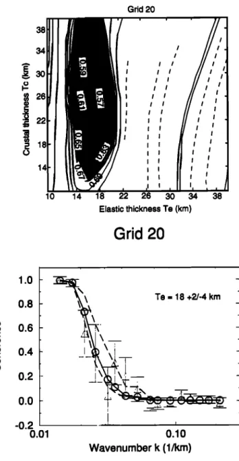
respectively, were assumed for each subregion. As an independent check on our T c estimates, we varied the crustal thickness from 10 to 40 km in each region. The best fitting elastic plate thickness for each subregion is obtained by minimising the residuals between the observed and predicted coherence. After a series of tests on grid 21 (the Adamawa uplift) where constraints on the Moho depth exist from seismic refraction data [Stuart et al., 1985], we estimated the residuals by a one-norm misfit method [e.g., Parker and McNutt, 1980]. It is important to note that the misfit error estimated in this case is higher than that reported in earlier studies [e.g., Bechtel et al., 1987]. Table 2 shows a listing of the physical parameters used to estimate the observed and predicted coherence for all the subregions.

Description of Coherence Models

The observed coherence and the best fit model of computed coherence for the 33 subgrids are shown in Figure 7. These plots allow comparison between elastic plate thickness beneath active and inactive volcanic areas, sedimentary basins and cratonic subregions. For all the grids, the coherence is close to zero at short wavelengths and gradually approaches 1 at long wavelengths where the plate is weak and deflected by surface and/or subsurface loads. At short wavelengths, the plate is strong enough to support topographic loads with no corresponding Bouguer gravity anomalies. The transition from low to high coherence occurs within a narrow wave band, with large error bars caused by wavenumber averaging in fall- Table 2. Physical Parameters Used for the Estimation of the

Observed and Predicted Coherence

Parameters Definitions Value Z m or T c Moho depth, depth to

subsurface load

Pc average crustal density

Pm upper manfie density

g gravity acceleration

G gravitational constant

E Young's modulus v Poisson's ratio

T e effective elastic thickness

D flexural rigidity 10-40 km 2670 kg m -3 3300 kg m -3 9.8 m s -2 6.67 x 10'tim • kg-ts '2 1 x 10 • N m '2 0.25 inverted E Te • [12(1-v2)] 4

off wave bands. As discussed below, the transition may be more broad and show scatter, indicating that the region considered is not uniformly rigid (e.g., Figure 7, grid 7). In that case, the resulting coherence represents an average of subregions with different flexural rigidities weighted by the product of the powers of gravity and topography. Comparing the observed and predicted coherence allows us to determine the flexural rigidity and thus the effective elastic thickness; evidently, the transitional wave band is shifted to longer wavelengths with increasing flexural rigidity [Forsyth, 1985]. The coherence models for grids 1, 2, 3, and 4 have to be interpreted with care because of a lack of data in these areas. Thus, while computing an elastic thickness map, these values are rejected. For grids 30, 31, 32, and 33, the coherence is not well constrained and the values are also rejected. The T e values obtained for each region and the corresponding root-mean- square (rms) errors are listed on Table 3.

Error Estimations of Te

Several methods can be used to estimate the errors on T e values. The common way is to find the minimum and maximum values of T e that fit the same number of points in the fall-off wave band, as the best fitting coherence model [e.g., Ebinger et al., 1989]. In this study, we used a different approach. For each grid, T e and T c are varied within a range of values, and the best fitting model corresponds to the (T e , T c) couple with the smallest rms error which measures the residual between the observed and predicted coherence. The results show that the rms errors lie between 0.55 and 1.83 (Table 3). The lower value corresponds to grid 20 located at the Benue trough axis, while the highest error is obtained for grid 6, the eastern part of Chad basin. Since both parameters are varied, we can draw, for each grid, arms error contour map for T c versus T e. After we have selected the best fitting model (Te), the shaded region in each rms error contour drawing sets the upper and lower confidence limits for T e (Figure 8). The minimum rms residual is increased by no more than 0.12 to give the rms contour for the limits to T e. This approach is illustrated in Figure 8, and the minimum and maximum T e curves for the three selected grids (20, 2,6 and 5) are also shown. For the first contour map (Figure 8a, grid 20), the best fitting model gives a T e value of 18 km (with T c = 28 km), the minimum is 14 km and the maximum is 20 km. Thus the T e value for this grid is 18 +2/-4 km. Figure 8b (grid 26) shows that the best fitting model corresponds to a T e of 30 km (T c =