THEORETICAL EVOLUTION OF OPTICAL STRONG LINES ACROSS COSMIC TIME

HAL Id: hal-02994121

https://hal.archives-ouvertes.fr/hal-02994121

Submitted on 7 Nov 2020

HAL is a multi-disciplinary open access

archive for the deposit and dissemination of

sci-entific research documents, whether they are

pub-lished or not. The documents may come from

teaching and research institutions in France or

abroad, or from public or private research centers.

L’archive ouverte pluridisciplinaire HAL, est

destinée au dépôt et à la diffusion de documents

scientifiques de niveau recherche, publiés ou non,

émanant des établissements d’enseignement et de

recherche français ou étrangers, des laboratoires

publics ou privés.

STRONG LINES ACROSS COSMIC TIME

Lisa J. Kewley, Michael A. Dopita, Claus Leitherer, Romeel Davé, Yuan

Tiantian, M Allen, Brent Groves, Ralph Sutherland

To cite this version:

Lisa J. Kewley, Michael A. Dopita, Claus Leitherer, Romeel Davé, Yuan Tiantian, et al..

THEORET-ICAL EVOLUTION OF OPTTHEORET-ICAL STRONG LINES ACROSS COSMIC TIME. The Astrophysical

Journal, American Astronomical Society, 2013, 774 (2), pp.100. �10.1088/0004-637X/774/2/100�.

�hal-02994121�

THEORETICAL EVOLUTION OF OPTICAL STRONG LINES ACROSS COSMIC TIME

Lisa J. Kewley

Australian National University and University of Hawaii

Michael A. Dopita

Australian National University and King Abdulaziz University

Claus Leitherer STScI Romeel Dav´e University of Arizona Tiantian Yuan University of Hawaii Mark Allen University of Strasbourg Brent Groves Leiden University and Ralph Sutherland

Australian National University Draft version April 26, 2013

ABSTRACT

We use the chemical evolution predictions of cosmological hydrodynamic simulations with our latest theoretical stellar population synthesis, photoionization and shock models to predict the strong line evolution of ensembles of galaxies from z = 3 to the present day. In this paper, we focus on the brightest

optical emission-line ratios, [NII_{]/Hα and [O}III_{]/Hβ. We use the optical diagnostic}

Baldwin-Phillips-Terlevich (BPT) diagram as a tool for investigating the spectral properties of ensembles of active galaxies. We use four redshift windows chosen to exploit new near-infrared multi-object spectrographs. We predict how the BPT diagram will appear in these four redshift windows given different sets of assumptions. We show that the position of star-forming galaxies on the BPT diagram traces the ISM conditions and radiation field in galaxies at a given redshift. Galaxies containing AGN form a mixing sequence with purely star-forming galaxies. This mixing sequence may change dramatically with cosmic time, due to the metallicity sensitivity of the optical emission-lines. Furthermore, the position of the mixing sequence may probe metallicity gradients in galaxies as a function of redshift, depending on the size of the AGN narrow line region. We apply our latest slow shock models for gas shocked by galactic-scale winds. We show that at high redshift, galactic wind shocks are clearly separated from AGN in line ratio space. Instead, shocks from galactic winds mimic high metallicity starburst galaxies. We discuss our models in the context of future large near-infrared spectroscopic surveys.

Subject headings: galaxies:starburst—galaxies:abundances—galaxies:fundamental parameters

1. _INTRODUCTION

Understanding how galaxies formed and evolved is one of the primary drivers of modern astronomical research. Measuring the fundamental properties of galaxies as a function of cosmic time is now possible by combining

[email protected]

spectroscopy from the world’s largest telescopes with state-of-the-art theoretical simulations.

The collisionally excited emission-lines provide key di-agnostics of the gas-phase chemical abundance, the ization state of the gas, the dust extinction, and the ion-izing power source of the galaxy. Baldwin et al. (1981)

(com-monly referred to as the BPT diagram) can be used to classify galaxies dominated by AGN from those domi-nated by star formation. Star-forming galaxies form a tight abundance sequence on the BPT diagram (Dopita & Evans 1986; Dopita et al. 2000). The location of the

star-forming abundance sequence on the [NII_]/Hα

ver-sus [O III_{]/Hβ diagram at a given redshift probes (1)}

the spread in global metallicity of the observed star-forming galaxy population, (2) the stellar ionizing ra-diation field of the star-forming population, and (3) the conditions of the interstellar medium (ISM) surrounding

the star-forming regions. Therefore, the [NII_{]/Hα versus}

[OIII_{]/Hβ diagram can be used as a tool for}

investigat-ing the metallicity and ionizinvestigat-ing radiation field in star-forming galaxies as a function of cosmic time, indepen-dent of the large systematic errors that plague the chem-ical abundance scale (Kewley & Ellison 2008; Bresolin et al. 2009; Kudritzki et al. 2012).

Galaxies containing an Active Galactic Nucleus (AGN) are easily separated from purely star-forming galaxies us-ing the BPT diagram. The extreme ultra-violet (EUV) “hard” radiation field from the accretion disk of an AGN

ionizes the [O III_{] and [N} II_{] lines, producing larger}

[OIII_{]/Hβ and [N}II_{]/Hα line ratios than usually seen in}

star-forming galaxies. Osterbrock & Pogge (1985) and Veilleux & Osterbrock (1987, hereafter VO87) derived the first semi-empirical AGN classification schemes for the BPT diagram based on a combination of observa-tions and and photoionization models. These diagnos-tics were refined by Kewley et al. (2001b) using stellar population synthesis, photoionization and shock models. Power-law AGN models show that position and spread of the AGN region on the BPT diagram traces the metal-licity in the extended narrow-line region of AGN (Groves et al. 2004b).

Clearly, the gas-phase metallicity has a critical influ-ence on the location of both star-forming galaxies and AGN on the BPT diagram. Both theory and observa-tions indicate that the mean metallicity of star-forming galaxies rises with cosmic time (e.g., Nagamine et al. 2001; De Lucia et al. 2004; Kobulnicky & Kewley 2004; Kobayashi et al. 2007; Maiolino et al. 2008; Dav´e et al. 2011a; Yuan et al. 2012; Zahid et al. 2012). The metal-licity evolution of galaxies will therefore change the po-sition of galaxies on the BPT diagram as a function of redshift. Because optical classification of starburst and AGN is based on either empirical fits to local galaxies, or theoretical models developed for local galaxies, cur-rent BPT classification methods may not be applicable at high redshift.

Testing BPT classification methods at intermediate or high redshift has been difficult in the past. At z > 0.4,

the [N II_{] and Hα lines are redshifted into the}

near-infrared. With single-slit near-infrared spectroscopy,

[NII_{]/Hα and [O}III_{]/Hβ ratios have now been observed}

for small numbers of individual galaxies at high redshift (Teplitz et al. 2000; Finkelstein et al. 2009; Hainline et al. 2009; Bian et al. 2010; Rigby et al. 2011; Yabe et al.

2012). Stacked [NII_{]/Hα and [O}III_{]/Hβ ratios of large}

numbers of galaxies have also been measured (Erb et al. 2006), and the first large NIR spectroscopic surveys are now being conducted (Trump et al. 2013, e.g.,).

The majority of galaxies at z > 0.4 show an offset

to-wards larger [N II_{]/Hα and [O} III_{]/Hβ ratios compared}

with local galaxies. This offset may be caused by a higher (2×) ionization parameter in high redshift galaxies. A larger ionization parameter may be produced by high nebular electron densities, a higher rate of star formation, a top-heavy initial mass-function (IMF), a high volume filling factor, and a large escape fraction of UV photons (Brinchmann et al. 2008b). Lehnert et al. (2009) sug-gest that the offset results from high gas densities and pressures that are similar to the most intense nearby SF regions locally, but spread over scales of 10-20 kpc in high redshift galaxies. Higher electron densities and ionization parameters have been measured for several high redshift galaxies (Hainline et al. 2009; Bian et al. 2010; Liu et al. 2008), but a large electron density by itself cannot ex-plain the offset in all cases (see Rigby et al. 2011). Groves et al. (2006) use photoionization models to show that the emission-line ratios in some high redshift galaxies could be explained by a combination of starburst and AGN ac-tivity. A similar conclusion was reached by Trump et al. (2011) after combining HST spectra with Chandra X-ray data for a sample of galaxies at z ∼ 2. Concurrent star-formation and AGN activity has also been found in some high redshift lensed galaxies (Wright et al. 2010).

The astronomical community is now on the cusp of ob-taining the BPT diagnostic emission lines for large sam-ples of z > 0.4 galaxies for the first time, thanks to new near-infrared multi-object spectrographs. New near in-frared multi-object spectrographs include MOSFIRE on Keck (McLean et al. 2010), FMOS on Subaru (Kimura et al. 2010), MMIRS on Magellan (McLeod et al. 2004), and FLAMINGOS II on Gemini (Eikenberry et al. 2008). These near-infrared multi-object spectrographs will al-low the ionizing source in galaxies to be analyzed as a function of redshift in statistically significant numbers of galaxies, for the first time.

To interpret these new observations, a theoretical un-derstanding of how the key BPT features may change at high redshift is needed. Such an understanding is essential for separating samples of star-forming galaxies from AGN at high redshift, and for tracking fundamental physical properties of the active galaxy population with redshift. This theoretical understanding is now achiev-able through modern cosmological hydrodynamic simu-lations, stellar evolution and photoionization models.

In this paper, we combine the predictions of cosmolog-ical hydrodynamic simulations models with stellar evo-lution, photoionization and shock models to predict how the BPT diagram may change with redshift. In Section 2, we describe the theoretical chemical evolution predic-tions used. Our simulapredic-tions for the star-forming galaxy abundance sequence are given in Section 3. In Section 4, we model how the the line ratios of galaxies containing AGN may evolve with redshift. Section 5 gives theoreti-cal predictions of the position of the BPT diagram within specific redshift windows. We investigate contamination from shocks, and we discuss the limitations of this work. Our conclusions are presented in Section 6. Throughout this paper, we adopt the flat Λ-dominated cosmology as measured by the 7 year WMAP experiment (h = 0.72,

Ωm= 0.29; Komatsu et al. 2011).

2. _{CHEMICAL EVOLUTION OF ACTIVE GALAXIES}

We utilize the chemical evolution estimates from Dav´e et al. (2011b,a). The Dav´e et al. (2011b) models use

the GADGET-2 N-body + Smoothed Particle Hydrody-namic code (Springel et al. 2005) in a ΛCDM cosmology. This code incorporates gas cooling and heating processes, including the effects of metal line cooling (Oppenheimer & Dav´e 2006). Density-driven star formation is calcu-lated using a Schmidt law (Schmidt 1959). Chemical en-richment from Type II supernovae, Type I supernovae, and AGB stars is included. Dave et al. use a Monte Carlo approach to model galactic outflows, where the mass loss due to outflows is related to the star formation rate and a variable mass loading factor.

We use the predicted evolution in the gas-phase

chem-ical abundance for galaxies with stellar mass M∗ >

109_M

⊙ across 0 < z < 3. We parameterize the relative

change in chemical abundances, ∆(log O/H), from z = 0 to an arbitrary redshift z by a 3rd order polynomial:

∆(log O/H) = −0.0013 − 0.2287z + 0.0627z2−0.0070z3.

(1) This equation applies to star-forming galaxies with

M∗ > 109M⊙ (chosen to avoid Malmquist bias). The

1σ error about equation 1 is ±0.1 dex at z = 0, falling to ±0.05 dex at z=3.

Equation 1 assumes that there is no mass dependence

in the chemical evolution for M∗ > 109M⊙ and over

0 < z < 3. Theory suggests that more massive galaxies undergo more rapid enrichment than less massive galax-ies due to additional contributions from wind recycling (Dav´e et al. 2011a). However, we show in Yuan et al. (2012) that equation 1 fits the slope of the current

metal-licity history of galaxies for M∗ > 109M⊙ to within the

observational errors. In future, when the chemical en-richment history of galaxies as a function of stellar mass is understood, a mass term could be included in equa-tion 1.

3. _{THE STAR-FORMING ABUNDANCE SEQUENCE}

We combine stellar evolutionary synthesis models with our MAPPINGS III photoionization models to generate theoretical limits to the expected ionizing radiation field as a function of redshift. We have tested this combina-tion of stellar populacombina-tion synthesis and photoionizacombina-tion models extensively for local star forming galaxies (e.g., Kewley et al. 2001a; Levesque et al. 2010). Zero-age and

1 Myr old models are able to reproduce the [N II_]/Hα

and [OIII_{]/Hβ line ratios in the majority of star-forming}

galaxies. However, the [SII_{]/Hα and [O}I_{]/Hα line ratios}

require a harder ionizing radiation field than is available in current stellar population synthesis models (Levesque et al. 2010). This situation may be resolved when the effects of stellar rotation are incorporated into the stel-lar evolutionary tracks used by the population synthesis models. Initial investigations into the effect of stellar rotation on the ionizing radiation field at solar metallic-ity is promising (Levesque et al. 2012). Until the full set of stellar tracks with rotation become available, we

limit our analysis of BPT evolution to the [N II_]/Hα

and [O III_{]/Hβ emission-line ratios which can already}

be reproduced using current stellar population synthesis models.

3.1. _{The Local Star-forming Abundance Sequence}

The Starburst99 (SB99) models that we use are de-scribed in detail in Levesque et al. (2010) and Nicholls et al. (2012). Briefly, we apply a Salpeter IMF (Salpeter

1955) with an upper mass limit of 100 M⊙. The

choice of IMF makes negligible difference on the opti-cal emission-line ratios used in this analysis. We use the Pauldrach/Hillier model atmospheres, which em-ploy the WMBASIC wind models of Pauldrach et al. (2001) for younger ages when O stars dominate the lu-minosity (< 3 Myr), and the CMFGEN atmospheres from Hillier & Miller (1998) for later ages when Wolf-Rayet (W-R) stars dominate. These stellar atmosphere models include the effects of metal opacities. We use the Geneva group “high” mass-loss evolutionary tracks (Meynet et al. 1994). These tracks include enhanced mass-loss rates that are applicable to low-luminosity W-R stars and can reproduce the blue-to-red supergiant ra-tios observed in the Magellanic Clouds (Schaller et al. 1992; Meynet 1993). Starburst99 generates a synthetic FUV spectrum using isochrone synthesis (e.g., Charlot & Bruzual 1991), in which isochrones are fitted to the evolutionary tracks across different masses rather than discretely assigning stellar mass bins to specific tracks. We use the zero-age instantaneous burst models because these models provide the best fit to the SDSS star-forming galaxy sequence at z ∼ 0 (Dopita et al. 2013). To match the nebular metallicities of our photoionization code, we interpolate between the STARBURST99 model grids as a function of metallicity.

We use our Mappings IV photoionization code (Binette et al. 1985; Sutherland & Dopita 1993; Dopita et al. 2013) to model the interstellar medium surrounding the SB99 ionizing radiation field. We assume the solar abundance set of Asplund et al. (2005). This abundance set in-cludes revised solar abundances for key elements, includ-ing oxygen and carbon. As in Levesque et al. (2010), the α-element abundances are assumed to scale linearly with metallicity, with the exception of Helium and Nitrogen. For helium, we include the stellar yield in addition to the primordial abundance from Pagel et al. (1992). For nitrogen, we assume primary and secondary nucleosyn-thetic components as measured by Mouhcine & Lan¸con (2002) and Kennicutt et al. (2003). The resulting N/H ratio is parameterized in Groves et al. (2004a). Metals are depleted out of gas phase and onto dust grains. The dust depletion factors are given in Groves et al. (2006), and are based on Kimura et al. (2003), who examined the metal absorption along several lines of sight within the local interstellar cloud.

Mappings uses either a plane parallel or spherical ge-ometry with the ionization parameter defined at the ini-tial edge of the nebula. For a spherical geometry, an ef-fective ionization parameter q can be defined that takes into account the spherical divergence of radiation at the

Stromgren radius Rs(Str¨omgren 1939):

qef f =

QH0

4πRs2nH

(2)

where QH0 is the flux of ionizing photons above the

Lyman limit. If the thermal gas only occupies a fraction of the available volume, the ionization parameter can be defined in terms of a volume filling factor.

and can be thought of as the maximum velocity ioniza-tion front that an ionizing radiaioniza-tion field is able to drive through a nebula. This dimensional ionization parame-ter is related to the dimensionless ionization parameparame-ter U through the identity U ≡ q/c. The dimensional ioniza-tion parameter is typically −3.2 < log U < −2.9 for local

HII_{regions (Dopita et al. 2000) and star-forming}

galax-ies (Moustakas 2006; Moustakas et al. 2010). In practice, all models with a similar effective ionization parameter produce very similar spectra, assuming all other param-eters are held constant (e.g., Dopita et al. 2000).

To minimize small uncertainties produced by particu-lar geometries, we calculate spherical models in which q is determined at the inner radius. The average ionization parameter is lower than this initial value, and is depen-dent on the ionization parameter of the initial radius.

Models were run with pressure P/k = 105.5_cm−3 _K,

where k is the Boltzmann constant. In an ionized nebula,

electron temperatures are ∼ 104_{K, yielding a density of}

10 − 30 cm−3_{, typical of giant extragalactic HIIregions.}

Detailed photoionization, excitation, and recombination are calculated at increments (step size 0.03) throughout the nebula. The model completes when the hydrogen gas is fully recombined. A full description of the

mod-els, including geometry, is given in L´opez-S´anchez et al.

(2012).

Unlike the Kewley & Dopita (2002) models, our cur-rent models include a sophisticated treatment of dust, including the effects of absorption, grain charging, ra-diation pressure, and photoelectric heating of the small grains (Groves et al. 2004a). The latest version of Map-pings incorporates a Kappa temperature distribution that is a more realistic representation of the electron tem-perature distribution in a turbulent ISM than a Stefan-Boltzmann distribution (Nicholls et al. 2012).

Figure 1 (left panel) shows our model grid in com-parison to the local star-forming galaxy sequence from the Sloan Digital Sky Survey (SDSS) from Kewley et al. (2006b). The SDSS galaxies were selected within the redshift range of 0.04 < z < 0.1 to minimize aperture effects and Malmquist bias (Kewley et al. 2004).

We fit an equation of the form log[OIII]/Hβ = a

log([NII]/Hα)+b+c to our model grid, where a, b, c are con-stants. This polynomial form was chosen for consistency with previous fits to theoretical model grids, including the hard ionizing radiation field from the P`egase stellar population synthesis models (Kewley et al. 2001a; Kauff-mann et al. 2003). According to our models, the mean position of a galaxy along the local star-forming sequence is

log([OIII]

Hβ ) =

0.61

log(N II/Hα) + 0.08+ 1.1 (3)

In Figure 1 (right panel), we show the polynomial fit from equation 3. This polynomial represents the mean local star-forming abundance sequence with model

es-timated errors of ±0.1 dex in both the [N II_{]/Hα and}

[O III_{]/Hβ directions. The upper and lower bounds of}

±0.1 dex (dashed lines) encompass 91% of the SDSS

star-forming galaxies.

The [NII_{]/Hα and [O} III_{]/Hβ line ratios along}

equa-tion 3 are related to metallicity through the following equation

12 + log O/H = 8.97 − 0.32x, (4)

where x = log[OIII]/Hβ_{[N II]/Hα} and metallicity is defined on

the Kewley & Dopita (2002) metallicity scale. We note that the following analysis depends only on the relative change in metallicity along the local starburst abundance sequence (equation 3). Different metallicity diagnostics have systematic offsets in their absolute abundance scale but relative metallicity measurements are conserved to within ±0.03 dex on average (Kewley & Ellison 2008). Thanks to this conservation of relative metallicities, the relative change in position along equation 3 is indepen-dent of the metallicity calibration used.

3.2. _{Factors that affect the Star-Forming Abundance}

Sequence

Individual galaxies that lie on the BPT diagram at high redshift are likely to evolve off the BPT diagram before z = 0. Thus, an observed change in the star-forming abundance sequence will track the change in in-trinsic galaxy properties across the star forming galaxy population at different epochs.

The position of our theoretical star-forming galaxy abundance sequence is determined by: (1) the shape of the ionizing radiation field, (2) the geometrical distribu-tion of gas with respect to the ionizing sources, (3) the metallicity range, and (4) the electron density (pressure) of the gas. We discuss the effect of changing each of these quantities below.

3.2.1. _{Shape of the Ionizing Radiation Field}

The stellar ionizing radiation field may change with redshift as a result of a change in the fraction of ionizing photons produced by the young stellar population. In a pure star forming galaxy, the hardness of the ionizing radiation field is related to the slope of the IMF, the age of the stellar population and the metallicity of the galaxy. A stellar population with a shallow initial mass function produces a hard ionizing radiation field, but there is no solid evidence for a change in IMF with redshift (see Bastian et al. 2010; Greggio & Renzini 2012).

The stellar population age is directly related to the shape of the ionizing radiation field. Hard ionizing ra-diation fields can be produced at ∼ 3 − 5 Myr when the stellar population may be dominated by Wolf-Rayet stars (e.g., Schaerer 1996; Kehrig et al. 2008). Broad

HeII _{λ1640 emission has been observed in stacked}

spec-tra of Lyman Break Galaxies (Shapley et al. 2003) and in some individual high redshift gravitationally lensed galaxies (Cabanac et al. 2008; Dessauges-Zavadsky et al.

2010). The broad He II _{feature has been attributed to}

a significant contribution from O and Wolf-Rayet stars to the ionizing EUV radiation field at low metallicity (Brinchmann et al. 2008a). We note that radiative shocks

can produce a narrow, nebular He II feature (Dopita

et al. 2011; Lagos et al. 2012) which may be blended with the broad component produced in stellar atmospheres of luminous stars. Such blending could be difficult to dis-tinguish at high redshift.

A hard ionizing radiation field has been linked with low metallicity in star forming galaxies (e.g., Campbell et al. 1986; Galliano et al. 2005; Madden et al. 2006; Hunt et al.

-2.0

-1.5

-1.0

-0.5

0.0

0.5

LOG ([NII]/H

α

)

-1.0

-0.5

0.0

0.5

1.0

1.5

LOG ([OIII]/H

β

)

-2.0

-1.5

-1.0

-0.5

0.0

0.5

LOG ([NII]/H

α

)

Figure 1. The [NII]/Hα versus [OIII]/Hβ optical diagnostic diagram for the Sloan Digital Sky Survey galaxies analyzed by Kewley et al. (2006b). Left: The colored curves show our new theoretical stellar population synthesis and photoionization model grid for star-forming galaxies based on a κ electron temperature distribution. Right: The red solid curve shows the mean star-forming sequence for local galaxies. The shape of the red solid curve is defined by our theoretical photoionization models, while the position is defined by the best-fit to the SDSS galaxies. The ±0.1 dex curves (dashed lines) represent our model errors and contain 91% of the SDSS star-forming galaxies. 2010; Levesque et al. 2010). There are several potential

reasons for the correlation between metallicity and the hardness of the ionizing radiation field:

(1) High energy photons produced by metal-rich stars are absorbed by metals in the stellar atmosphere, known as metal blanketing. The preferential absorption of high energy photons yields a softer ionizing radiation field (e.g., Gonz´alez Delgado et al. 2005).

(2) The Hayashi track shifts to hotter effective temper-atures at low metallicities, enabling metal-rich massive stars to maintain a higher effective temperature com-pared with metal-poor stars of similar spectral types (Elias et al. 1985; Levesque et al. 2006).

(3) Low metallicities correspond to lower mass loss rates, allowing low metallicity stars to remain on the main sequence for longer timescales (Meynet et al. 1994; Maeder & Conti 1994).

(4) In isolated stars, rotational mixing causes heavy mass loss. This mass loss produces bluer colors in the red supergiant phase, lowering the mass limit required for a star to enter the Wolf-Rayet phase (Levesque et al. 2012). Thus, a population of rotating massive stars will contain a larger fraction of hot, massive stars to contribute ioniz-ing photons to the stellar radiation field. This rotational hardening is a function of metallicity, with more signif-icant hardening in metal-poor environments (Leitherer

2008).

(5) In binary stars, efficient mass-transfer can spin-up the rotation of the companion star, causing similar mix-ing effects as in rotatmix-ing isolated stars (de Mink et al. 2009; Eldridge & Stanway 2012). Whether a rapidly rotating star can spin down depends on stellar winds, which are weaker at low metallicities due to metal opac-ity. Rotation and binarity are not yet included in stellar population synthesis models for a range of metallicities.

A hard ionizing radiation field can also be produced by contamination from an active galactic nucleus or ra-diative shocks. Slow shocks (100-200 km/s) associated with galactic-scale winds have been observed both locally (Rich et al. 2010, 2012) and at high redshift (Yuan et al. 2012). We address these two possibilities in Section 4 and Section 5.1.

It is unclear whether high redshift star-forming galax-ies have a harder radiation field than local galaxgalax-ies at the same metallicity. If a harder ionizing radiation field

exists in high redshift galaxies, both the [OIII_{]/Hβ and}

[NII_{]/Hα line ratios will be affected. A larger fraction of}

photons with energies above the ionization potentials of

[NII_{] and [O}III_{] will raise the [N}II_{]/Hα and [O}III_]/Hβ

line ratios because there are more photons available to

ionize nitrogen and oxygen. The [O III_{] emission-line is}

ionizing radiation field than [NII_{] because the difference}

in ionization potentials is large (35eV c.f. 14.5eV). In Figure 2, we illustrate the effect of raising the hardness of the ionizing radiation field in galaxies along the local abundance sequence (orange dashed line). The harder ra-diation field moves the entire abundance sequence above and to the right on the BPT diagram. A harder ionizing radiation field could account for part (or all) of the large

[NII_{]/Hα and [O}III_{]/Hβ ratios seen at high redshift.}

-2.0 -1.5 -1.0 -0.5 0.0

0.5

LOG ([NII]/H

α

)

-1.0

-0.5

0.0

0.5

1.0

1.5

LOG ([OIII]/H

β

)

Figure 2. An illustration of the effect of varying different galaxy parameters on the star-forming galaxy abundance sequence in the [NII]/Hα versus [OIII]/Hβ diagnostic diagram. The original SDSS star-forming galaxy sequence is well-fit by the red theoretical curve. Raising the hardness of the ionizing radiation field (orange dashed line) moves the abundance sequence towards larger [NII]/Hα and [OIII]/Hβ ratios. A similar effect is seen when the electron den-sity of the gas is raised (green dot-dashed line). The relationship between ionization parameter, metallicity and the [N II]/Hα and [OIII]/Hβ line ratios is more complex. At high metallicities, rais-ing the ionization parameter causes the [NII]/Hα ratio to become smaller, while [OIII]/Hβ is largely unaffected. At low metallicities, raising the ionization parameter raises the [OIII]/Hβ ratio while [NII]/Hα is largely unaffected.

3.2.2. _{Geometrical distribution of the gas}

The geometrical distribution of the gas around the ion-izing source can be changed by shocked stellar winds.

Stellar winds clear ionized gas from the interior of an HII

region. Because highly ionized species, such as [O III_],

form preferentially at the inner radii of H II _regions,

shocked stellar winds will lower the effective ionization parameter of the nebula (Yeh & Matzner 2012).

Our theoretical photoionization models assume a uni-form medium, where the geometrical distribution of the gas is approximated by a volume filling factor. In reality,

H II _{regions may be clumpy and porous. Ultracompact}

HIIregions in the Milky Way contain a porous

interstel-lar medium (Kurtz et al. 1999; Kim & Koo 2001).

Ra-dio observations indicate that young HII _{regions in low}

metallicity galaxies also have a clumpy and porous

dis-tribution of gas (Johnson et al. 2009). A clumpy, porous medium allows some ionizing photons to escape the neb-ula without being absorbed by the interstellar gas. In this scenario, the effective ionization parameter may be lowered, depending on the escape fraction and the optical thickness of the porous medium.

Our models are calculated for radiation-bounded HII

regions. In the radiation-bounded scenario, the model

finishes when hydrogen is completely recombined. If HII

regions are density bounded (i.e. the H II _region

den-sity is sufficiently low that the stars can ionize the entire

nebula), the [OIII_{] ionization zone is likely to be largely}

unaffected, but the [N II_{] excitation and Hydrogen}

re-combination zones may be shortened. Therefore, the

[OIII_{]/Hβ ratio may be larger, while the [N}II_{]/Hα ratio}

will be similar to or smaller than observed in a

radiation-bounded nebula. Since the [O II_{] zone is shorter in a}

density-bounded nebula, the [OIII_]/[OII_{] ratio becomes}

larger. If radiation-bounded models are applied to such

nebulae, then the larger [OIII_]/[OII_{] line ratio would be}

interpreted as a high ionization parameter.

Detailed ionization parameter mapping of the HII

re-gions in nearby galaxies can constrain whether the H II

regions are radiation bounded or density bounded. A

mixture of radiation-bounded and density-bounded HII

regions have been observed in the local group (Pellegrini et al. 2012). Nakajima et al. (2012) suggest that

Lyman-α emitters at high redshift contain density-bounded HII

regions. It is unclear whether density-bounded nebulae are common in normal star-forming galaxies, either lo-cally or at high redshift.

The geometrical distribution issues described above can be considered in terms of an effective ionization pa-rameter. We discuss the effect of changing the ionization

parameter on the [NII_{]/Hα and [O}III_{]/Hβ line ratios in}

Section 3.2.5.

3.2.3. _{The Metallicity Range of Galaxies}

The spread in metallicity across a galaxy sample deter-mines the length of the star-forming abundance sequence. Galaxy samples that span a small range of metallicities occupy only a portion of the star-forming abundance se-quence. For example, interacting or merging galaxies typically have lower central metallicities due to large-scale gas infall (Kewley et al. 2006a, 2010; Rupke et al. 2010b; Ellison et al. 2010; Rich et al. 2012; Scudder et al. 2012). On the other hand, low metallicity galaxies, such as blue compact dwarfs, occupy the highest positions (lowest metallicities) on the star-forming abundance se-quence (Levesque et al. 2010).

The metallicity range of high redshift galaxies is un-known. Samples selected from rest-frame blue colors or the Lyman break may be missing a population of faint, low metallicity galaxies and a population of dusty, metal-rich star forming galaxies. Gravitationally lensed sam-ples probe fainter galaxy samsam-ples and a broader range of metallicities, within current instrumentation detection limits (see Figure 5 in Yuan et al. 2012, for a compari-son of current instrumentation detection limits for lensed and non-lensed samples).

3.2.4. _{The Electron Density}

In an isobaric density distribution, the density is de-fined in terms of the ratio of the mean ISM pressure, P ,

and mean electron temperature, Te, through ne = _TPek.

For an ionized gas, the electron temperature is ∼ 104 _K

and the density is simply determined by the ISM pres-sure.

The SDSS abundance sequence is fit by our

pho-toionization models with an electron density of ne =

10 − 102_cm−3_{, typical of local HII regions (Osterbrock}

1989). Brinchmann et al. (2008b) shows that the dis-tance away from the star-forming abundance sequence correlates strongly with electron density; SDSS

galax-ies with larger electron densitgalax-ies (ne = 102 cm−3) lie

above and to the right of the mean SDSS star-forming abundance sequence. Highly active star-forming galax-ies, such as warm infrared galaxies and luminous infrared

galaxies have dense ionized gas (102₋₁₀3_cm−3_{; Kewley}

et al. 2001b; Armus et al. 2004) and lie above and to the right of the SDSS star-forming abundance sequence (Yuan et al. 2010).

Many high redshift galaxies also have dense nebular

gas (∼ 103 _cm−3_{) (e.g. Brinchmann et al. 2008b;}

Hain-line et al. 2009; Bian et al. 2010; Rigby et al. 2011; Wuyts et al. 2012a) and galaxies with high Hα surface bright-ness (Lehnert et al. 2009; Le Tiran et al. 2011). Fig-ure 2 shows the effect of raising the electron density from

ne = 10 cm−3 (solid red line) to ne = 1000 cm−3

(dot-dashed green line). Both the [O III_{]/Hβ and [N} II_]/Hα

ratios are larger at higher electron densities due to the increased rate of collisional excitation. We conclude that high electron densities could account for at least part of

the enhanced [N II_{]/Hα and [O}III_{]/Hβ ratios observed}

in current samples of high redshift galaxies.

3.2.5. _{Ionization Parameter}

Much previous research into the differences between high redshift and local galaxy emission-line ratios has focused on the ionization parameter (Brinchmann et al. 2008b; Liu et al. 2008; Hainline et al. 2009). The ion-ization parameter is a useful tool for comparisons among

H II _{regions or galaxies because it can be readily}

mea-sured using the ratio of high ionization to low

ioniza-tion species of the same atom (such as [O III_]/[O II_]).

However, it is important to understand the fundamental physical properties that govern the ionization parameter. The ionization parameter is determined by the hydrogen ionizing photon flux, and the pressure of the interstellar medium.

The number of hydrogen ionizing photons per unit area can be changed by either scaling the ionizing radiation field (i.e. raising or lowering the luminosity of the stel-lar population) or by modifying the shape (hardness) of the ionizing radiation field. Because the ionization parameter, electron density and radiation field hardness are interrelated, isolating the cause(s) of a shift towards

larger [N II_{]/Hα and/or [O} III_{]/Hβ ratios at high}

red-shift is non-trivial. Furthermore, different geometrical gas distributions can mimic a higher or lower observed ionization parameter. Several of these processes may contribute to the observed ionization parameter in star-forming galaxies.

Local galaxies with high measured or inferred ion-ization parameters include Wolf-Rayet galaxies (Brinch-mann et al. 2008b), strong Hα emitter galaxies (Shim & Chary 2012), and low metallicity galaxies (Kewley et al.

2007). In Wolf-Rayet galaxies, the high ionization pa-rameter is caused by the shape of the ionizing radiation field produced in Wolf-Rayet atmospheres with line

blan-keting (Gonz´alez Delgado et al. 2002). Strong Hα

emit-ting galaxies may have high ionization parameters due to a high ISM pressure (Brinchmann et al. 2008b; Shim & Chary 2012), and/or low metallicity.

The ionization field can be scaled by raising the star

formation rate of a stellar population. High redshift

galaxies typically have larger star formation rates than local galaxies (Shapley et al. 2005; Hainline et al. 2009). Hainline et al. (2009) suggest that these larger star for-mation rates may lead to a larger reservoir of ionizing photons, leading to a higher ionization parameter.

Alternatively, a large ionization parameter may be a natural consequence of a low metallicity environment. The shape of the ionizing radiation field is a strong function of time since the most recent burst of star

formation. The shape of the ionizing radiation field

is also determined by the fraction of ionizing photons that are either absorbed by the stellar atmospheres and surrounding gas, and conversely, the fraction of ionizing photons that escape the nebula without being absorbed by ISM. These effects combine to produce a correlation between ionization parameter and metallicity (Dopita & Evans 1986; Dopita et al. 2000; Kewley & Dopita

2002). Dopita et al. (2006) show theoretically that

the ionization parameter inversely correlates with the

metallicity of an HII_{region, Z, according to q ∝ Z}−0.8_.

The reason for this correlation is twofold;

(1) At high metallicity, the stellar wind opacity is larger. This large opacity absorbs a greater fraction of the ionizing photons, reducing the ionization parameter

in the surrounding HII_region.

(2) At high metallicity, stellar atmospheres scatter the photons emitted from the photosphere more efficiently. This scattering efficiently converts luminous energy flux into mechanical energy flux at the base of the stellar wind. The reduced luminous energy flux available to

ionize the surrounding HII _{region is observed as a lower}

ionization parameter.

Many high redshift galaxies have high ionization pa-rameters (−2.9 < log U < −2.0 Pettini et al. 2001; Lemoine & Pelletier 2003; Maiolino et al. 2008; Hain-line et al. 2009; Erb et al. 2010; Richard et al. 2011; Wuyts et al. 2012a). Nakajima et al. (2012) compare the ionization parameter and metallicity (as traced by

the [O III_]/[O II_{] vs R23 line ratios) for a large sample}

of high redshift galaxies, including Lyman Break, lensed, and Lyman-α emitting galaxies. Their comparison shows that the majority of high redshift galaxies have simi-lar ionization parameters to local galaxies at the same metallicity. Thus, the high ionization parameters at high redshift may simply be a natural consequence of a low metallicity environment.

The effect of ionization parameter on the [N II]/Hα

and [OIII_{]/Hβ ratios depends on the metallicity regime.}

Figure 1 (left panel) shows that at low metallicities

(log([N II_{]/Hα)< −0.9), a larger ionization parameter}

will raise the [O III]/Hβ ratio, while the [N II]/Hα

ra-tio remains constant within ±0.2 dex. At high

metallici-ties (log([NII_{]/Hα)> −0.7, a larger ionization parameter}

roughly constant (to within ±0.1 dex). This effect is il-lustrated in Figure 2. For the metallicities of most high redshift galaxies (log(O/H) + 12 < 8.6; Erb et al. 2006; Wuyts et al. 2012b; Yuan et al. 2012), a high

ioniza-tion parameter will raise the [OIII_{]/Hβ ratio such that}

high redshift galaxies will lie above the local abundance sequence, as observed. Therefore, a high ionization

pa-rameter can account for part of the large [OIII_{]/Hβ and}

[NII_{]/Hα ratios observed in high redshift galaxies.}

3.3. _{The High Redshift Star-forming Abundance}

Sequence

Although a hard ionizing radiation field is linked with low metallicity, it is unclear whether hard ionizing ra-diation fields are a feature of high redshift star-forming galaxies. Figure 2 shows that the combination of a larger ionization parameter at low metallicity and a higher elec-tron density may mimic the effects of a harder ionizing ra-diation field. Rest-frame UV spectroscopy of high metal-licity galaxies at z > 2 is needed to determine whether

the large [N II_{]/Hα and [O} III_{]/Hβ ratios seen in high}

redshift galaxies are caused by a higher electron den-sity and ionization parameter or the combined effects of a higher electron density, ionization parameter, and a harder EUV ionizing radiation field.

Further, selection biases may be limiting the current range of electron densities and ionization parameters

ob-served at high redshift. The combination of surface

brightness dimming and current observational sensitiv-ities limits high redshift samples to galaxies with high emission-line surface brightness. This limit biases sam-ples towards galaxies with high star formation rates

(SFR> 4M⊙/yr), and more intense star formation.

Lo-cal starburst galaxies are characterized by higher

pres-sures than normal H II _{regions (Kewley et al. 2001b).}

High pressures of 106 _{< P/k < 10}7 _{implies gas}

densi-ties of 100 − 1000 cm−3_{. A greater fraction of starburst}

galaxies in high redshift samples would produce larger

[N II_{]/Hα and [O} III_{]/Hβ ratios when compared with}

local samples of normal star-forming galaxies.

Gravitationally lensed samples can probe an order of magnitude fainter in star formation rate (SFR >

0.4M⊙/yr; Richard et al. 2011). Consequently,

gravita-tionally lensed samples cover a larger range of [NII_]/Hα

and [O III_{]/Hβ ratios than non-lensed samples}

(Hain-line et al. 2009; Richard et al. 2011; Wuyts et al. 2012a). However, current lensed samples still do not sample the full range of star formation rates seen in the global spectra of local normal star forming galaxies ( SFR

> 0.01 M⊙/yr Kewley et al. 2002). A statistically

signif-icant sample of high redshift galaxies that covers a broad range of metallicity and stellar mass is required to

deter-mine the full range of [N II_{]/Hα and [O} III_{]/Hβ ratios}

at high redshift. Until such samples are available, we as-sume a lower limit and an upper limit to the star forming abundance sequence at high redshift (z ∼ 3).

3.3.1. _{Lower Limit Abundance Sequence (Normal SF} conditions)

Our lower limit abundance sequence is calculated as-suming that galaxies at a given redshift have the same shape EUV radiation field, the same range of electron densities, and the same relationship between metallicity

and ionization parameter as local star-forming galaxies. In this very conservative scenario, the star-forming abun-dance sequence is given by equation 3. Chemical evolu-tion moves galaxies down along the star-forming galaxy

sequence towards smaller [O III_{]/Hβ ratios and larger}

[NII_{]/Hα ratios.}

3.3.2. _{Upper Limit Abundance Sequence (Extreme SF} conditions)

We use PEGASE 2 models (Fioc & Rocca-Volmerange 1999) to provide the upper limit to the ionizing radiation field at z = 3. These models provide the hardest radia-tion field because the models use the Clegg et al. (1992) planetary nebula nucleus (PNN) atmospheres for stars with high effective temperatures (T > 50, 000K). Clearly, the ionizing spectrum of active star-forming galaxies is dominated by the emission from the atmospheres of mas-sive stars, not planetary nebulae. However, we use the PNN atmospheres as a substitute for massive star stellar atmospheres, in the absence of the full suite of stellar atmospheres with the effects of stellar rotation. The PE-GASE 2 models use the Padova tracks (Bressan et al. 1993) and the OPAL opacities (Iglesias et al. 1992). The application of PEGASE 2 with our Mappings III code is described in detail in Kewley et al. (2001a).

If we assume that the hard radiation field sets the up-per limit at z = 3 for star-forming galaxies, then the evo-lution of the star-forming abundance sequence between 0 < z < 3 follows

log([OIII]/Hβ) = 1.1 + 0.03z

+ 0.61

log([NII]/Hα) + 0.08 − 0.1833z.(5)

This upper limit is consistent with the limit that we derive from a combination of a larger ionization

param-eter (−2.9 < log U) and larger electron density (Ne ∼

1000 cm−3_{) for metallicities below log(O/H) + 12∼ 8.8.}

According to our models, the metallicity of a galaxy at redshift z on the star-forming abundance sequence given by equation 5 is

12 + log O/H = 8.97 + 0.0663z −

log(O3N 2)(0.32 − 0.025z) (6)

where O3N 2 = [OIII]/Hβ/[NII]/Hα.

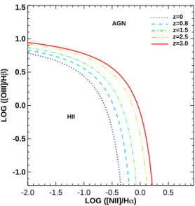
In Figure 3, we show the evolution of the upper limit star-forming abundance sequence with redshift given by

equation 5. Figure 3 should not be used over small

redshift intervals with small samples to test the evolu-tion of the galaxy populaevolu-tion because the model errors (±0.1 dex) and spread in ionization parameter log(U ), (±0.1 dex) at a given redshift are larger than the pre-dicted evolution of the sequence for an ensemble of galax-ies across each redshift interval.

3.3.3. _{Abundance Sequence Shape}

The metallicity range (or spread) of the star-forming population determines the length of the abundance se-quence. In cosmological hydrodynamic simulations, the evolution of the lower metallicity bound is dominated by chemical enrichment of the most metal poor galaxies

-2.0 -1.5 -1.0 -0.5 0.0 0.5 LOG ([NII]/Hα) -1.0 -0.5 0.0 0.5 1.0 1.5 LOG ([OIII]/H β ) z=0 z=0.8 z=1.5 z=2.5 z=3.0 HII AGN

Figure 3. The BPT diagram showing the theoretical lower limit (z = 0; blue dot-dashed line) and upper limit star-forming abun-dance sequence as a function of redshift (z = 0.8, 1.5, 2.5, 3.0; dashed, dot-dashed, triple dot-dashed and solid lines, respectively). in the galaxy population. The upper metallicity bound may be influenced by gas inflows from the intergalactic medium such that the upper metallicity bound might fall with redshift (Nagamine et al. 2001).

Again, we assume that at least some galaxies at z ∼ 3 have reached the level of enrichment of galaxies in the local universe, and we assume that the mean metallicity of the galaxy population evolves according to equation 1. The scatter of galaxies about the abundance sequence is dominated by the range in ionization parameters and electron densities in the galaxy population at a given redshift. How the spread in these properties changes with redshift is unknown. For simplicity, we assume that the spread in these properties about the mean is constant with redshift and is ±0.1 dex.

4. _{THE MIXING SEQUENCE}

Local active galaxies form two branches on the BPT diagram. While pure star-forming galaxies lie along the abundance sequence, galaxies with a contribution from a non-thermal radiation field form a sequence that extends towards the pure AGN region of the BPT diagram (i.e.

towards large [NII_{]/Hα and [O}III_{]/Hβ ratios). This}

se-quence can be produced by either a mixture of gas ionized by hot stars and gas ionized by an AGN (Groves et al. 2004b), or a mixture of gas ionized by hot stars and gas ionized by radiative shocks (Kewley et al. 2001a; Allen et al. 2008). We therefore refer to this sequence as the mixing sequence, where mixing refers to the mixture of a soft photoionizing radiation field from star-formation and a hard non-thermal radiation field from either AGN or shocks. In this section, we focus on starburst-AGN mixing. We investigate starburst-shock mixing in Sec-tion 5.1.

4.1. _{AGN Models}

The [N II_{]/Hα and [O} III_{]/Hβ line ratios of a galaxy}

purely ionized by an AGN are influenced by the metal-licity of the surrounding narrow-line region, the shape

of the AGN ionizing radiation field (characterized by a power-law), and the ionization parameter. We use the Mappings III dusty, radiation pressure dominated mod-els of Groves et al. (2004a).

These models use the same abundance set and deple-tion factors as our starburst models (Secdeple-tion 3.1). The ionizing spectrum is based on a power-law,

Fµ∝µα (7)

where the frequency µ is defined over 5eV < µ < 1000eV with four values of the power-law index α (−1.2, −1.4, −1.7, −2.0).

The shape of the ionizing radiation field may change with metallicity; a smaller fraction of metals and dust may change the AGN torus structure and potentially

alter the accretion disk. Unfortunately, the effect of

metallicity on the AGN ionizing radiation field is un-known. For simplicity, we assume the same ionizing spec-tral shape for all metallicities.

In isobaric radiation-pressure dominated models, the local density varies continually throughout the models. In this case, the hydrogen density is defined as the

den-sity of the [SII_{] emission zone, which is located close to}

the ionization fronts in the Narrow Line Region (NLR). In this zone, we assume that the electron density is

nH = 103cm−3.

The total radiative flux entering the narrow line re-gion cloud is determined by the ionization parameter,

UN L defined at the inner edge of the nebula. The

ion-ization parameter range is 0.0 < log(UN L) < −4.0 with

intervals of −0.3, −0.6, and −0.1 dex. The NLR models are truncated at a column density of log[N(H I)] = 21, consistent with observations of NLR clouds (Crenshaw et al. 2003).

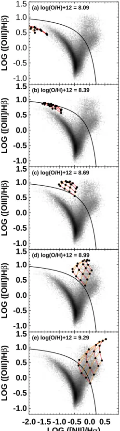
In Figure 4, we show the position of the dusty radiation-pressure dominated AGN models as a func-tion of metallicity on the BPT diagram. The posifunc-tion of the AGN models changes substantially with metallic-ity. At low metallicity, the AGN models move towards

lower [NII_{]/Hα ratios and the spread in [O}III_{]/Hβ ratios}

becomes smaller. The reason for this effect is twofold; (1) at low metallicity, nitrogen shifts from a secondary nucle-osynthetic element to a primary nuclenucle-osynthetic element, and (2) the rise in electron temperature offsets the fall in oxygen abundance, yielding a roughly constant mean

[OIII_{]/Hβ ratio as a function of metallicity.}

Figure 4 indicates that it will be impossible to dis-tinguish low metallicity galaxies containing AGN (i.e. metallicities log(O/H) + 12. 8.4) from low-metallicity star-forming galaxies using the BPT diagram.

A sample of AGN galaxies at a given NLR metallicity may span a range of ionization parameter and power-law indices. We therefore use the full suite of ionization pa-rameter and power-law indices to define our 100% AGN region on the BPT diagram. We have tested these pho-toionization models for local galaxies containing AGN; the models produce remarkable agreement with the ob-served position of AGN on the BPT diagram (Allen et al. 1998; Groves et al. 2004b; Kewley et al. 2006b).

4.2. _{AGN Metallicity}

Figure 4 indicates that AGN reside in metal-rich gas in the local universe (9.0 < log(O/H) + 12 < 9.3; KD02

-1.0

-0.5

0.0

0.5

1.0

1.5

LOG ([OIII]/H

β

)

-1.0

-0.5

0.0

0.5

1.0

1.5

LOG ([OIII]/H

β

)

-1.0

-0.5

0.0

0.5

1.0

1.5

LOG ([OIII]/H

β

)

-1.0

-0.5

0.0

0.5

1.0

1.5

LOG ([OIII]/H

β

)

-2.0 -1.5 -1.0 -0.5 0.0 0.5

LOG ([NII]/H

α

)

-1.0

-0.5

0.0

0.5

1.0

1.5

LOG ([OIII]/H

β

)

Figure 4. The (Groves et al. 2004a) dusty radiation pressure dom-inated photoionization models for AGN as a function of metallic-ity. Lines of constant ionization parameter (orange) and constant power-law index (red) are shown. For comparison, the SDSS sam-ple from (Kewley et al. 2006b) is shown.

scale). Indeed, low metallicity AGN are extremely rare in local galaxies (Groves et al. 2006). The star form-ing abundance sequence and the AGN region on the BPT diagram are linked together by a “mixing sequence” which can be modelled by a combination of starburst and power-law AGN photoionization models (e.g., Groves

et al. 2004b). The overlap region between the

star-forming abundance sequence and the AGN mixing se-quence provides an additional constraint on the metal-licity of local galaxies containing AGN. The local SDSS mixing sequence extends from only the most metal-rich star-forming galaxies (9.0 < log(O/H) + 12 < 9.2) to the AGN region. It is not clear whether AGN are only found in the most metal rich galaxies at higher redshift.

The combination of metallicity gradients and surface brightness dimming may affect the observed metallicity of galaxies along the mixing sequence. The narrow-line region surrounding an AGN is typically 1-5 kpc (Ben-nert et al. 2006), smaller than the typical radius sam-pled by global spectra of local pure star-forming galaxies (∼ 8 kpc on average; Kewley et al. 2004). Therefore, in galaxies with very steep metallicity gradients, the AGN narrow-line region may be more enriched than the ex-tended star-forming regions which probe a larger radius, on average. For example, a steep metallicity gradient

(−0.15 dex kpc−1_{) can produce a 0.2 dex metallicity}

dif-ference from spectra measured within circular apertures of 1 kpc and 5 kpc. On the other hand, a flat metal-licity gradient would give the same metalmetal-licity for the star-forming gas and the NLR, regardless of the size of the star-forming and narrow-line regions. Flat metallic-ity gradients can be produced by large-scale gas flows triggered by galaxy interactions (Kewley et al. 2006a, 2010; Rupke et al. 2010b; Rich et al. 2012). Theory in-dicates that metallicity gradients systematically flatten after first pericenter and flatten again during final coa-lescence (Rupke et al. 2010a; Torrey et al. 2012). The metallicity gradient can be steepened by a late nuclear starburst, providing that outflows have not already re-moved a substantial fraction of the nuclear star-forming gas (Torrey et al. in prep).

We note that local disk galaxies with typical gradients

(−0.04 ± 0.09 dex kpc−1 _{Zaritsky et al. 1994; van Zee}

et al. 1998; Rupke et al. 2010a) are unlikely to produce a large difference in the NLR and star forming regions. Local early-type galaxies have even shallower gradients (Henry & Worthey 1999).

Current observations of metallicity gradients at high redshift are limited by small numbers and low angular resolution observations. Metallicity gradients in some high redshift lensed isolated star-forming galaxies appear to be significantly steeper than local galaxies (Yuan et al. 2011; Jones et al. 2013), but in other high redshift galax-ies, the gradients appear to be flat or inverted (Cresci et al. 2010; Swinbank et al. 2012; Queyrel et al. 2012). The steepest gradients were obtained by observing grav-itationally lensed galaxies with integral field spectro-graphs with laser-guided adaptive optics (Jones et al. 2010; Yuan et al. 2011; Jones et al. 2013). Observational issues such as poor angular resolution (> 0.1”F W HM ) or low S/N can lead to weak line smearing which sys-tematically flattens or inverts metallicity gradients that are intrinsically steep (Yuan et al. 2013). In the absence of robust observational or theoretical constraints on the

cosmic evolution of the metallicity gradient in galaxies, we consider two extreme cases:

• Case 1: Metal-rich NLRThe AGN narrow line

region at z = 3 has reached the level of enrichment seen in the narrow line region of local galaxies. This extreme case implies that galaxies at high redshift have a steeper metallicity gradient on average than observed in local galaxies. In this scenario, the metallicity gradient of galaxies would flatten with time until z = 0.

• Case 2: Metal-poor NLRThe AGN narrow line

region at z = 3 is at the same average metallicity as the surrounding star-forming gas. This extreme case implies a flat metallicity gradient on average at high redshift. If the average galaxy metallicity gradient is flat at high redshift, the gradient steep-ens with time until z = 0. .

We interpolate between the model grids in Figure 4 to

derive the range of possible [NII_{]/Hα and [O}III_]/Hβ

ra-tios for the 100% AGN region at each redshift. The AGN model metallicity is simply the local average metallicity (log(O/H) + 12∼ 9.0) for Case 1. For Case 2, the aver-age AGN model metallicity is determined by the redshift through equation 1. The spread of the 100% AGN region on the BPT diagram for both cases is determined by the full range of ionization parameters and power-law indices in our model grid at a given AGN model metallicity.

We derive starburst-AGN mixing sequences for each redshift using our AGN and starburst models. For both cases, we assume that AGN reside in the most metal-rich galaxies at any epoch, as observed locally. We assume that the fraction of the starburst sequence that inter-sects the AGN mixing sequence covers the top 0.2 dex in metallicity. If this assumptiondoes not hold at high redshift, then we would expect to see galaxies to the left

of our mixing sequence (i.e. towards lower [NII_{]/Hα line}

ratios than spanned by the mixing sequence). We fit the mixing sequences with a 2nd or 3rd order least-square polynomial:

y = a + bx + cx2+ dx3 (8)

where y = log [OIII]/Hβ and x = log [NII]/Hα. The constants a − d are given for each mixing line bound-ary at each redshift in Table 1, along with the range of

[N II_{]/Hα and [O} III_{]/Hβ values over which the mixing}

sequences are defined. The four scenarios tabulated in Table 1 are described in detail in Section 5.

5. _{THE COSMIC BPT DIAGRAM}

With our theoretical predictions for the star-forming abundance sequence and the AGN mixing sequence, we can predict how the the BPT diagram might appear at different redshifts. We have two extreme cases for the star-forming galaxies and two extreme cases for the AGN NLR metallicity, which we briefly summarize below.

Star forming galaxies at high redshift (z = 3) may have ISM conditions and/or an ionizing radiation field that are the same as local galaxies (normal ISM conditions) or that are more extreme than local galaxies (extreme ISM conditions). Extreme conditions in star-forming galaxies can be produced by either a larger ionization parameter

and a more dense interstellar medium, and/or a harder ionizing radiation field.

The AGN narrow line region at high redshift may have reached the level of enrichment seen in local galax-ies (metal-rich), or it may evolve similarly to the star-forming gas. In the latter case, the AGN narrow-line region at high redshift would be more metal-poor than local AGN narrow-line regions.

Combining our two sets of extreme cases gives four limiting scenarios for the position of galaxies on the BPT diagram at each redshift:

• Scenario 1: Normal ISM conditions, and

metal-rich AGN NLR at high-z.

• Scenario 2: Normal ISM conditions, and

metal-poor AGN NLR at high-z.

• Scenario 3: Extreme ISM conditions, and

metal-rich AGN NLR at high-z.

• Scenario 4: Extreme ISM conditions, and

metal-poor AGN NLR at high-z.

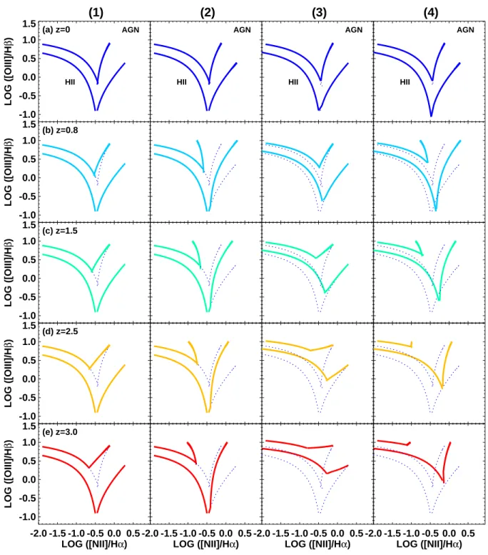
In Figure 5, we show how the abundance sequence and the mixing sequence are expected to evolve with redshift given our four limiting scenarios (columns 1-4 in Fig-ure 5). The local SDSS sequence boundaries are shown for reference (blue dashed lines). We discuss the predic-tions given by each limiting scenario individually below.

Scenario 1: In this scenario, we have assumed that the

ISM conditions (and/or the ionizing radiation field) are constant as a function of redshift, and the AGN NLR at z = 3 has already reached the level of enrichment seen in local AGN NLRs. Therefore, the only change to the po-sition of galaxies on the BPT diagram is a broadening of the mixing sequence at the intersection with the abun-dance sequence. This broadening is due to the lower mean and larger range of metallicities in star-forming galaxies at higher redshift.

Scenario 2: In this picture, we have assumed that the

ISM conditions (and/or the ionizing radiation field) are constant as a function of redshift, and that the AGN NLR metallicity evolves with time in the same way that pure star-forming galaxies evolve (equation 1). This im-plies that AGN galaxies at z = 3 would have flat metal-licity gradients that steepen with time. At high

red-shift, the mixing sequence occupies lower [N II_]/Hα

ra-tios than local galaxies due to the metallicity sensitivity

of the [NII_{]/Hα ratio. The 100% AGN region is broad in}

this scenario, spanning a large range of [NII_{]/Hα ratios}

(−1.0 <[NII_{]/Hα< 0). The breadth of the AGN region}

illustrates the effect of differing AGN power-law indices and ionization parameters at lower metallicities.

Scenario 3: Here, we have assumed that the the

ioniz-ing radiation field or the ISM conditions in star formioniz-ing galaxies become more extreme at high redshift, and that the AGN NLR at z = 3 has already reached the level of enrichment seen in local AGN NLRs (i.e. a steep metal-licity gradient at high-z). In this scenario, the position of the star-forming abundance sequence rises from z = 0

to z = 3 towards larger [OIII]/Hβ ratios, while the AGN

mixing sequence becomes shorter. At z = 3, the abun-dance sequence and AGN mixing sequence form almost a single horizontal sequence across the BPT diagram. If

Table 1

Mixing Sequence Boundariesa

Scenario 1 Scenario 2 Scenario 3 Scenario 4

SF model: normal SF model: normal SF model: extreme SF model: extreme

AGN model: Metal-rich NLR AGN model: Metal-poor NLR AGN model: Metal-rich NLR AGN model: Metal-poor NLR

z= 0 z= 0 z= 0 z= 0

lower upper lower upper lower upper lower upper

a 0.034 0.885 0.029 0.885 0.031 0.917 0.029 0.917 b 1.447 -0.792 1.340 -0.792 1.441 -0.491 1.332 -0.491 c -0.986 -6.712 -0.712 -6.712 -0.879 -6.090 -0.710 -6.090 d . . . 1.472 . . . 1.594 xr [-0.45, 0.29] [-0.45 , -0.12] [-0.45 , 0.29] [-0.45 , -0.12] [-0.50 , 0.29] [-0.44 , -0.12] [ -0.47 , 0.29] [-0.44 , -0.12] yr [-0.90 , 0.38] [ -0.20 , 0.91] [ -0.90 , 0.38] [ -0.20 , 0.91] [ -0.90 , 0.38] [ -0.10 , 0.91] [ -1.05 , 0.38] [ -0.10 , 0.91] z= 0.8 z= 0.8 z= 0.8 z= 0.8

lower upper lower upper lower upper lower upper

a 0.034 1.002 0.603 -13.734 0.025 1.032 0.567 -6.277 b 1.447 0.602 1.422 -38.844 1.429 0.882 1.728 -18.664 c -0.986 -2.078 -1.606 -25.672 -0.693 -1.382 -2.702 -11.999 d . . . 5.072 . . . 6.479 xr [ -0.45 , 0.29] [ -0.54 , -0.12] [ -0.45 , 0.30] [ -0.77 , -0.59] [ -0.37 , 0.29] [ -0.49 , -0.12] [ -0.34 , 0.30] [ -0.77 , -0.56] yr [ -0.90 , 0.38] [ 0.05 , 0.91] [ -0.90 , 1.00] [ 0.13 , 1.00] [ -0.60 , 0.38] [ 0.26 , 0.91] [ -0.85 , 1.00] [ 0.40 , 1.00] z= 1.5 z= 1.5 z= 1.5 z= 1.5

lower upper lower upper lower upper lower upper

a 0.034 1.027 0.745 -10.585 0.047 1.022 0.696 -6.293 b 1.447 0.902 1.365 -26.300 1.252 0.939 1.955 -15.695 c -0.986 -0.837 -0.233 -14.970 -0.262 0.155 -3.789 -8.433 d . . . 10.3905 . . . 18.5499 xr [ -0.45 , 0.29] [ -0.61 , -0.12] [ -0.45 , 0.17] [ -0.88 , -0.67] [ -0.35 , 0.29] [ -0.55 , -0.12] [ -0.25 , 0.17] [ -0.88 , -0.71] yr [ -0.90 , 0.38] [ 0.16 , 0.91] [ -0.90 , 1.00] [ 0.25 , 1.00] [ -0.40 , 0.38] [ 0.55 , 0.91] [ -0.60 , 1.00] [ 0.60 , 1.00] z= 2.5 z= 2.5 z= 2.5 z= 2.5

lower upper lower upper lower upper lower upper

a 0.034 1.033 0.879 -8.604 0.163 0.958 0.834 -64.678 b 1.447 0.995 1.801 -19.285 0.722 0.415 2.479 -139.855 c -0.986 -0.246 4.277 -9.706 0.160 0.212 -3.271 -74.252 d . . . 20.374 . . . 58.818 xr [ -0.45 , 0.29] [ -0.67 , -0.12] [ -0.45 , 0.07] [ -0.99 , -0.75] [ -0.30 , 0.29] [ -0.70 , -0.12] [ -0.17 , 0.07] [ -1.01 , -0.99] yr [ -0.90 , 0.38] [ 0.25 , 0.91] [ -0.90 , 1.00] [ 0.37 , 1.00] [ -0.05 , 0.38] [ 0.77 , 0.91] [ -0.20 , 1.00] [ 0.85 , 1.00] z= 3.0 z= 3.0 z= 3.0 z= 3.0

lower upper lower upper lower upper lower upper

a 0.034 1.033 0.942 -8.212 0.259 0.933 0.908 2.037 b 1.447 1.005 2.268 -17.802 0.370 0.190 2.692 1.186 c -0.986 -0.109 7.423 -8.621 0.208 0.103 -0.839 0.171 d . . . 26.057 . . . 71.964 xr [ -0.45 , 0.29] [ -0.68 , -0.12] [ -0.45 , 0.04] [ -1.03 , -0.78] [ -0.28 , 0.29] [ -0.80 , -0.12] [ -0.15 , 0.04] [ -1.12 , -1.03] yr [ -0.90 , 0.38] [ 0.30 , 0.91] [ -0.90 , 1.00] [ 0.40 , 1.00] [ 0.16 , 0.38] [ 0.85 , 0.91] [ -0.10 , 1.00] [ 0.92 , 1.00] a

Mixing line boundaries extending from the star-forming abundance sequence (0% AGN) to the AGN region (100% AGN) on the BPT diagram. The coefficients a, b, c, d are defined according to y = a + bx + cx2

+ dx3

where y = log([OIII]/Hβ) and x = log([NII]/Hα). The range of x and y values (xr, yr) over which these polynomials are valid are shown. Scenarios (1-4) correspond to the 4 limiting scenarios for our theoretical models, described in Section 5 and shown as columns in Figure 5.

this scenario exists in high redshift galaxies, classifying galaxies into star-forming and AGN using the BPT dia-gram would be extremely difficult for z ≥ 2.5.

Scenario 4: In this scenario, we have assumed that

high redshift star forming galaxies have more extreme ISM conditions and/or a harder ionizing radiation field, and that the AGN NLR metallicity evolves with time in the same way that pure-star-forming galaxies evolve (i.e. a flat metallicity gradient at high redshift). According to these predictions, the star-forming abundance sequence rises at larger redshift, while the AGN mixing sequence become substantially broader and shorter. At z = 3, it would be extremely difficult to distinguish between high metallicity star-forming galaxies and galaxies containing AGN using the BPT diagram.

Figure 5 shows that distinguishing between these four scenarios is possible at specific redshifts. Scenarios (1) and (2) could be easily distinguished with intermediate or high redshift samples (z ≥ 0.8). All four scenarios

predict substantially different abundance and mixing se-quence positions at z ≥ 2.5. Thus, observations of the rest-frame optical emission-line ratios for statistically sig-nificant samples of active galaxies at z ≥ 2.5 are likely to yield important information on the ionizing radiation field and/or the ISM conditions in star-forming galaxies, as well as the nature of metallicity gradients in galaxies containing AGN at high redshift.

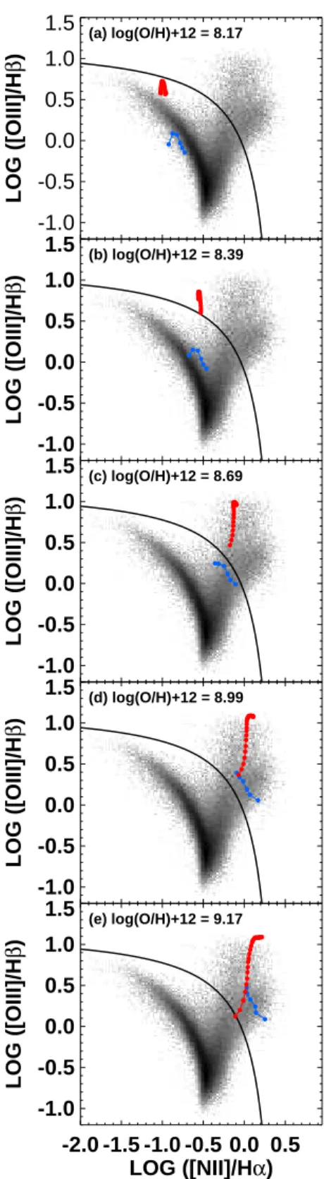
5.1. _{The Effect of Shocks}

Shocks associated with galactic winds may

substan-tially raise the [NII]/Hα emission-line ratio observed in

the global spectra of galaxies at high redshift. Radiative shocks are produced by a variety of astrophysical sources in galaxies, including starburst or AGN-driven outflows, cloud-cloud collisions from galaxy interactions, and jet-cloud collisions. In Rich et al. (2010) and Rich et al. (2011), we showed that outflows in infrared luminous galaxies can drive gas clouds into the ambient gas in the

(1)

(2)

(3)

(4)

Figure 5. The Cosmic BPT Diagram: Our theoretical predictions for the position of the star-forming abundance sequence (left curve) and the starburst-AGN mixing sequence (right curve). The primary driver for our BPT evolution model is chemical enrichment. The rows give the expected position of the two sequences as a function of redshift for four limiting model scenarios given in each column. Column (1): Normal ISM conditions, and metal-rich AGN NLR at high-z; Column (2): Normal ISM conditions, and metal-poor AGN NLR at high-z; Column (3): Extreme ISM conditions, and metal-rich AGN NLR at high-z; Column (4): Extreme ISM conditions, and metal-poor AGN NLR at high-z.