HAL Id: hal-03182960
https://hal.archives-ouvertes.fr/hal-03182960
Submitted on 27 Mar 2021
HAL is a multi-disciplinary open access
archive for the deposit and dissemination of
sci-entific research documents, whether they are
pub-lished or not. The documents may come from
teaching and research institutions in France or
abroad, or from public or private research centers.
L’archive ouverte pluridisciplinaire HAL, est
destinée au dépôt et à la diffusion de documents
scientifiques de niveau recherche, publiés ou non,
émanant des établissements d’enseignement et de
recherche français ou étrangers, des laboratoires
publics ou privés.
Surface-observed and satellite-retrieved cloudiness
compared for the 1983 ISCCP Special Study Area in
Europe
A. Henderson-Sellers, G. Seze, F. Drake, M. Desbois
To cite this version:
A. Henderson-Sellers, G. Seze, F. Drake, M. Desbois. Surface-observed and satellite-retrieved
cloudi-ness compared for the 1983 ISCCP Special Study Area in Europe. Journal of Geophysical Research,
American Geophysical Union, 1987, 92 (D4), pp.4019. �10.1029/JD092iD04p04019�. �hal-03182960�
JOURNAL OF GEOPHYSICAL RESEARCH, VOL. 92, NO. D4, PAGES 4019-4033, APRIL 20, 1987
Surface-Observed
and Satellite-Retrieved
Cloudiness
Compared for the 1983 ISCCP Special Study Area in Europe
1 G S•3ZE
2 F DRAKE,
1 AND M DESBOIS
2
A. HENDERSON-SELLERS,
.
,
.
.
A comparison has been undertaken between surface-observed total low- and high-cloud amount
and retrievals from METEOSAT radiance data made using the cluster technique of Desbois eli al.
(1982). The aim of the study was to establish whether surface-observed cloud information could
be usefully exploited to benefit satellite-based cloud retrievals. Observations from 124 surface stations at 1200 UT for the 20-day period from July 22 to August 10, 1983, were compared with retrievals made from METEOSAT radiances measured at 1130 UT. The comparisons for total and low-cloud amount are made for France and southern Britain. The high-cloud amount comparison was limited to 34 stations in southern Britain. The location and time period were selected to coincide with one of the regions designated for special study in the International Satellite Cloud
Climatology Project (ISCCP) (Schiffer, 1982). For total cloud amount, 29% of the retrievals were fully in agreement with the surface observations and 64% of differences were within •1 okra (•1 eighth of sky cover). In the case of layer cloud amounts, 64% of the low-cloud amount differences
and 50% of the high-cloud amount differences were within •1 okra, although many of these
successes (71% in the low-cloud amount) were for cases of totally clear or totally cloudy skies.
Surface observations, which offer the only source of accurate low-cloud amount evaluation in any multilayered situation, were found to identify thin cirrus which was not detected by the satellite retrieval and to detect small gaps in cloud decks and small clouds missed by the satellite retrieval. In addition, cloud retrievals in coastal locations seemed to be more successfully accomplished by surface observers than by the satellite retrieval algorithm used here, which does not take into account land-sea partition.
1. INTRODUCTION
It has been widely recognized that the radiative prop-
erties of clouds need to be better known and understood
[Global
Atmospheric
Research
Program
(GARP), 19781. To
this end a new global cloud climatology is at present being compiled under the auspices of the International SatelliteCloud Climatology
Project (ISCCP) [$chi•er, 1982; $chi•er
and Rossow,
1983, 1985]. This will be a 5-year archive,
be-
ginning in 1983, and is being compiled from satellite data. One of the stated objectives of the research component of ISCCP is "investigation of methods to infer additional cloudproperties
from satellite
observationsf
[Rossow
et al., 1985,
p. 901]. In order to achieve
such an objective
it is first es-
sential to establish which cloud properties are readily and successfully derivable from satellite data and which are lessaccessible. One approach is to compare results from a range
of different cloud retrieval algorithms. Such a comparison
(described
by Rossow
et al., [1985])
formed
the basis
for the
construction of the ISCCP algorithm. The fact that cloud fields are three-dimensional suggests an alternative, com-plementary
approach: comparison
of surface
(bottom-up)
and satellite (top-down) cloud
retrievals.
As part of the re-
search component of the ISCCP, a joint venture by United Kingdom and French scientists has focused on a comparisonof surface observations and satellite retrievals of clouds.
It must be recognized that the comparison described here
tilayered, overlapping, and dynamic cloud scene. In order to capture the fullest description of clouds, the best possi- ble approach might be the strategy adopted by the U.S. Air Force, which includes as much information as possi- ble: surface observations, satellite retrievals and aircraft re-
ports [Fye, !978]. On the other hand, this practice
leads
inevitably to heterogeneity
[e.g., Hughes
and Henderson-
Sellers,
1985]. Another way to help resolve
the dilemmas
of
insufficient data and ambiguous satellite retrievals is to ex- ploit additional information or retrieval methods only where they can improve the cloud characterization substantially. One example of this is to improve cloud cover and type eval-uation using
statistical
retrievals
for selected
scenes
[Rossow
et al., 1985]. In this paper, another question
is examined:
whether surface observations of clouds can be exploited toresolve ambiguities in satellite retrievals and to add lower- layer information unobtainable from satellites.
2. DATA 5OURCES AND METhODS or COMPARISON
2.1. Location and Timing
The location (France
and southern
Britain) and the time
period studied
(July 22 to August
10, 1983) were selected
to
coincide with one of the special study regions identified by ISCCP. Meteorologically, the 20-day period offers a range ofconditions typical of this region in the summertime. There
was an outbreak of Saharan dust from north Africa which
is not intended to be a validation exercise. Indeed the term spread over the Mediterranean Sea early in the period, while
"validation
• is hard to understand
in the context
of a mul- depression
systems
crossed
the northern
part of the region.
Beginning around ,luly 28, an anticyclone drifted in from
... the west to become established over the region, and it dom-
1Department
of
Geography,
University
of
Liverpool,
Liverpool,
inated
the
synoptic
conditions
for the
rest
of the
period.
England.
The
last
few
days
in July
saw
very
high
temperatures
over
2Laboratoire
de
M6t•orologie
Dynamiq•e,
Centre
National
de most
of Europe.
Cloud
types
were
varied,
including
ad-
la Recherche
Scientifique,
Palaiseau,
France•
vected
fog;
cumulonimbus
(especially
over
southern
France),
Copyright
1987
by the
American
Geophysical
Union.
frontal cloud,
and isolated
cirrus.
Paper
number
5D0383.
The method
of investigation
was twofold:
a straightfor-
0148-0227/87/006D-0383505.00 ward comparison of surface and satellite cloud retrievals pre.
4020 HENDERSON--SELLERS ET AL.: SURFACE AND SATELLITE CLOUDINESS FOR EUROPE IN 1983
ceded a detailed analysis of specific cases and features. Sec- tions 2 and 3 describe the data and preliminary results. In
section 4 these results are reviewed in the context of earlier
work, and proposals are made in section 5. 2.2. Surface Observatioas
Surface observations were supplied by the United Kingdom Meteorological Office and the Direction de la
Mtttorolo- gie de France. The observation stations used
were those
making round-the-clock
observations
(i.e., every
hour in the United Kingdom
and 3-hourly in France). These
stations were selected because it was believed that the ob-
servational data would be more likely to be consistent from such sources. Both the United Kingdom and France use
the okra code (eighths
of sky covered)
for reporting cloud
amount. However, in the United Kingdom, the number 9 is used to indicate sky obscured, whereas in France, the num- ber -9 is used to indicate that the sky is obscured or there isa datum missing, and the number-1 indicates a data prob-
lem. An attempt was made to exclude stations in which
these codes appeared; in the analyzed data they appear on only five separate occasions. Altogether, 124 stations were
used: 34 stations scattered over England and Wales and 90
located
in France (see Table 1).
For the French stations, only total and low-cloud amounts
were supplied, which confined the study of high-cloud
amount to the United Kingdom only. The amount of high
cloud was not supplied as such. Instead, information on the three lowest cloud layers is supplied. The layers are reported
in accordance
with the following
criteria: (1) the lowest
in-
dividual
layer of any amount;
(2) the next higher
individual
layer with an amount which is greater than or equal to 3okras; (3) the next higher individual layer with an amount
which is greater than or equal to 5 okras;
(4) if cumulonim-
bus is observed but not reported in the above categories, it is reported as a separate fourth category. Thus high cloud can fall in any or none of the first three categories, depend- ing upon the synoptic conditions. In order to obtain the high-cloud amount, any observations of a cloud at an alti- tude of 6 km or higher was considered to be a high cloud[Her Majest•t's
Stationat&t
Office
(HMSO), 1969]. The cloud
data used
in the comparison
are all midday (1200 UT) okra
cloud amounts for the period July 22 to August 10, 1983.2.3. Satellite Observations
The cloud amounts were derived from M•TEOSAT im-
of gravity and variances. Finally, each pixel of each of the 20 images is projected on the four-dimensional histogram
and is attributed to the class to which it is the nearest.
The use of variances allows separation of clouds which have similar spectral characteristics. Although classes with semi- transparent clouds or partial coverage of the pixels can be separated by the algorithm, pixels belonging to these classes have been considered as completely cloud covered. This is an important feature which has to be remembered in the following comparisons.
The area studied
here was split into five regions
(Figure
1). Although
the regions
overlap,
each station was assigned
to a particular region, as shown in Figure 1. The latitudesand longitudes of the comers of the regions are given in Table 2. The regions are larger in longitude than latitude, as the surface and atmospheric properties were thought to vary more with latitude than with longitude. There were five learning sets' one for each region.
2.4 Selection of the Comparison Areas
It was decided that an area 100 km by 100 km was the most useful for comparison purposes. Selection of this size was prompted by the identification by Barrett and Grant
[1979]
of the theoretical
maximum
radius of vision
of a sur-
face observer as 50 km and following detailed considerationof a range
of surface
observations
[e.g., Greenwood,
1985]. To
obtain the cloud amount in an area centered on each surface
station, all pixels within a box 100 km by 100 km (about
15 by 19 pixels) were attributed to one of the classes
in the
learning set for the appropriate region. Thus the percent-age coverage
of each class (cloud type) can be found, and
the total cloud amount can be calculated. The percentageto okra conversion used was
okra value = integer value of
[ (pe,ce,tage
x18•)
+ 0.5]
(1)
3. RESULTS OF INITIAL COMPARISON
3.1. Region- Wide Comparisons
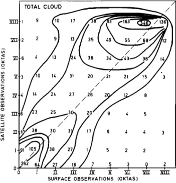
As a preliminary exercise, scattergraphs of numbers of
okra cloud retrievals made from the two platforms, surface and satellite, are shown in Figure 2. The total cloud dis-
tribution (Figure 2a) indicates
the strongly
bimodal
nature
of the retrievals. Both satellite and surface observations are
ages taken at 1130 UT each day. As the primary objective more likely to be •_6 oktas or _•1 okta than between 2 and was to establish whether surface observations could be used 5 okras. For the larger cloud amounts there is a clear ten- in selected situations to complement satellite data, only one dency for the satellite retrieval to be greater than the surface retrieval algorithm was used. The chosen algorithm, which observations by between 1 and 2 okras. However, this ten-
uses a clustering technique, is described by Desbois and Sdze dency is much less in the case of almost clear skies. In the
[1984]
and Sdze
and Desbols
[1986]
and will only be outlined case
of low-cloud
retrievals
(Figure
2b) the bimodal
feature
here. remains, although it is very much weaker, mostly because
The method combines spectral, spatial, and temporal in- there were very few occasions on which there were complete
formation. Each pixel of a chosen
image segment
is repre- low-level
overcasts.
The high-cloud
distribution
(Figure
2c)
sented
by four parameters:
two spectral ones (visible and contains
very many fewer observations,
as data are available
infrared values) and two spatial ones (local variances
corn- only for southern
Britain. The results are more noisy,
but
puted from the eight neighbors in the visible and infrared they show very characteristic features: surface observationsimages). First a four-dimensional
cumulative
histogram
is of zero okras
may correspond
to a wide range of high-cloud
built up for each segment for 10 of the 20 days. The clus- coverage by the satellite, from zero to 8 okras. The valuestering technique permits partitioning of this histogram, the are also rather scattered for the nonzero values of ground result being a separation of the histogram into classes rep- observations, with a general tendency to an overestimation
HENDERSON-SELLERS ET AL.: SURFACE AND SATELLITE CLOUDINESS FOR EU•tOPE IN 1983 4021
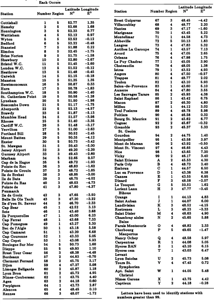
TABLE 1. Surface Stations Used With Latitude, Longitude, and the Region in Which
Each Occurs Station Latitude Longitude Number Region N ø E ø Cottishall 1 Hemsby 2 Honnington 3 Wattisham 4 Wyton 5 Bedford 6 Stansted 7 Elmdon 8 Brize Norton 9 Shawbury 10 Bristol W.C. 11 London W.C. 12 Heathrow 13 Gatwick 14 Manston 15 Herstmonceaux 16 Hurn 17 Southampton W.C. 18 St. Catherines Point 19 Lyneham 20 Boscombe Down 21 Aberporth 22 Brawdy 23 Mumbles Head 24 Rhoose 25 Cardiff W.C. 26 Yeovilton 27 Portland Bill 28 Mount Batten 29 Exeter 30 St. Mawgan 31 Jersey Airport 32 Gurnsey Airport 33 Marham 34 Cap de la Hague 35 Pointe du Roc 36 Pointe de Grouin 37 Ile de Brehat 38 Ile de Bat,. 39 Pointe du Ra,. 40 Pointe de 41 Penmarch Ile de Groix 42 Belle Ile Ole Tault 43
Ile d'yeu St. Saveur 44
Cap Bear 45 Sete 46 Ile Porquerolles 47 Cap Ferrat 48 Cap Pomegues 49 Bec de l'Aigle 50 Cap Camarat 51 Cap Couronne 52 Cap Cepet 53
Boulogne Sur Mer 54
Dieppe 55
Brest Tour Cesar 56 Bordeaux 57 Clermont Ferrand 58 Dijon 59 Limoges Bellgarde 60 Lyon Bron 61 Nimes-Couberssac 62 Agen 63 Perpignon 64 Alencon 65 Rennes 66 5 52.77 1.35 5 52.68 1.68 5 52.33 0.77 5 52.12 0.97 5 52.52 -0.12 5 52.22 -0.48 5 51.88 0.22 5 52.45 -1.75 5 51.75 -1.58 5 52.80 -2.67 5 51.45 -2.60 5 51.52 -0.12 5 51.48 -0.45 5 51.15 -0.18 5 51.35 1.35 5 50.87 O.33 5 50.78 -1.83 5 5O.9O -1.40 5 50.58 -1.28 5 51.50 -1.98 5 51.17 -1.75 5 52.13 -4.57 5 51.87 -5.13 5 51.57 -3.98 5 51.40 -3.35 5 51.48 -3.17 5 51.00 -2.63 5 50.52 -2.45 5 50.35 -4.12 5 50.73 -3.42 5 50.43 -5.00 3 49.20 -2.20 3 49.43 -2.60 5 52.65 0.57 5 49.72 -1.93 3 48.83 -1.62 3 48.72 -1.85 3 48.85 -3.00 3 48.75 -4.O2 3 48.03 -4.73 3 47.80 -4.37 3 47.65 -3.50 3 47.30 -3.22 3 46.70 -2.33 1 42.52 3.13 1 43.40 3.68 1 43.00 6.23 1 43.68 7.33 1 43.27 5.30 1 43.18 5.58 1 43.20 6.68 1 43.33 5.05 1 43.08 5.93 5 50.73 1.60 5 49.93 1.10 3 48.38 -4.48 2 44.83 -0.7O 2 45.75 3.17 4 47.27 5.08 2 45.87 1.18 2 45.72 4.95 1 43.75 4.4O 2 44.18 0.60 1 42.73 2.87 4 48.45 0.10 3 48.07 -1.72 TABLE 1. (continued) Latitude Longitude
Station Number Region N ø E ø
Brest Guipavas 67 3 48.45 -4.42 Villacoublay 68 4 48.77 2.20 Nantes 69 3 47.17 -1.60 Marignane 70 1 43.45 5.22 Montelimar 71 1 44.58 4.73 Abbeville 72 5 50.13 1.83 Langres 73 4 47.83 5.32 Antibes La Garoupe 74 1 43.57 7.13 Avord 75 4 47.05 2.65 Orleans 76 4 47.98 1.75 Le Puy Chadrac 77 1 45.05 3.90 Chateaudin 78 4 48.05 1.38 Istres 79 1 43.52 4.93 Angers 80 4 47.50 -0.57 Trappes 81 4 48.77 2.02 Toulon 82 1 43.10 5.93 Salon-de-Provence 83 1 43.60 5.10 Auxerre 84 4 47.80 3.55
Les Sauvages Tarare 85 2 45.93 4.38
Saint Raphael 86 1 43.42 6.75 Macon 87 2 46.30 4.80 Millau 88 I 44.12 3.02 Toul Posieres 89 4 48.78 5.98 Poitiers 90 4 46.58 0.32 Bourg St. Maurice 91 2 45.62 6.77 Cognac 92 2 45.67 -0.32 Grenoble 93 2 45.37 5.33 St. Geoirs Gourdon 94 2 44.75 1.40 Montpellier 95 1 43.58 3.97 Mont de Marsan 96 2 43.92 -0.50 Mont St. Vincent 97 4 46.65 4.43 Nice 98 1 43.65 7.20 Vichy 99 2 46.17 3.40 Saint Etienne A 2 45.53 4.30 Paris Orly B 4 48.73 2.40 Embrun C I 44.57 6.50 Luc en Provence D 1 43.38 6.38 Cannes E 1 43.55 6.95 Dinard F 3 48.58 -2.07 Le Touquet G 5 50.52 1.62 Lorient Lann H 3 47.77 -3.45 Bihoue Orange I I 44.13 4.83
Saint Auban •I I 44.07 6.00 Landivisiau K 3 48.52 -4.15 Rostrenen L 3 48.23 -3.33 Saint Dizier M 4 48.63 4.90 Chambray aixles N 2 45.65 5.88 Bains Parais Montsouris O 4 48.82 2.33 Cherbourg P 5 49.65 -1.47 Maupertus Nancy Ochey Q 4 48.58 5.97 Carpentras R 1 44.08 5.05 Hyeres BAN S I 43.10 6.15 Hyeres cem T 1 43.03 6.47 Levant Lyon Satolas U 2 45.73 5.08 Tours St. V 4 47.45 0.72 Symphorien Apt. Saint W 1 44.05 5.48 Christol Nimes Garons X 1 43.75 4.42 Captieux Y 2 44.18 -0.28
Letters have been used to identify stations with numbers greater than 99.
4022 HENDERSON-SELLERS ET AL.: SURFACE AND SATELLITE CLOUDINESS FOR EUROPE IN 1983
65 8•68B m 8Q9/I
67 L/.
o/.• 2H 66
80
V
78
76 84 73 •
59
'•'•'•
69
75
/.
•,,,•,
9O97
87•
92
58
99 85
A •9361
U N
91
7757
94
71
C
Y 63 88 ! RW .T96
95 6X2
79 7083
E
9B
•
64
/
46 52
49
5082
53%7D
T
5816
7/.
45,
Fig. 1. Map of northwest Europe, showing the five regions and distribution of the 124 surface stations which are identified by the numbers and letters listed in Table 1.
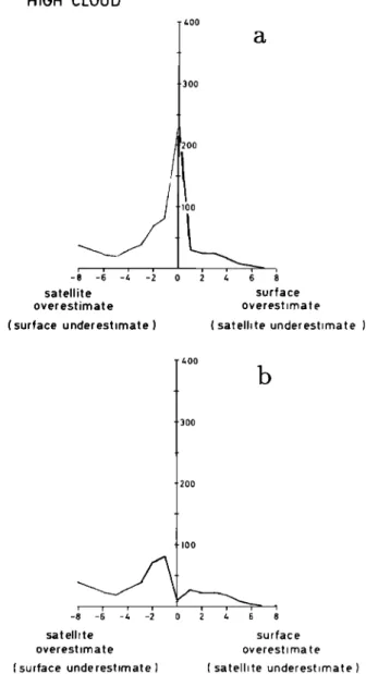
The okra differences between satellite and surface obser- vations at all locations and all times have been cumulated
into the frequency distributions shown in Figures 3a and 4a. The terminology adopted here is that a positive cloud amount difference is an apparent surface observer overes- timate and a negative cloud amount difference a satellite overestimate. These differences, of course, could be consid-
ered to be a satellite underestimate and a surface observer
underestimate, respectively. However, in this study they will initially be described in terms of overestimation. A zero represents an exact agreement between the surface-observed and satellite-retrieved cloud amount. Overall, for the 124 stations over the 20 days, the most frequent okra difference
is zero (Table 3). For total cloud, 28% of the differences
are
zero and 64% of them lie within •:1 okra. For low cloud,32% of the differences are zero and 64% lie within :/:1 okra. These results appear fairly positive, but many of these cases of good agreement are for totally clear or totally cloudy
skies. In the total cloud amount case, $$% of the zero okra
differences are due to agreement in totally clear or totally
cloudy situations. These conditions give rise to 71% of the
complete agreements in the case of low cloud. Additionally,
in the total cloud amount frequency distribution (Figure
3a), there.
is a tendency
for the satellite to overestimate,
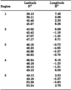
by approximately 1 okra. The low-cloud amount distribu-TABLE 2. The Latitudes and Longitudes of the Corners of the Five Regions
Shown in Figure 1
Latitude Longit ude
Region N ø E ø 1 39.13 7.45 39.11 2.08 45.49 2.33 45.57 8.36 2 43.50 8.09 43.42 -1.16 47.07 -1.25 47.17 8.71 3 46.19 -0.73 46.22 -4.95 49.96 -5.37 49.92 -0.79 4 46.24 6.16 46.19 -1.23 49.12 -1.31 49.13 6.56 5 49.13 2.52 49.16 -5.27 53.29 -5.83 53.24 2.78
HENDERSON-SELLERS ET AL.: SURFACE AND SATELLITE CLOUDINESS FOR EUROPE IN 1983 4023 TOTAL CLOUD 1 9 0 17 38 2 9 31 20 /21 21 / / 55 / / 24 27 26 8 / / 9 z, 5 25 / 30 3' 9 4 4 3 5 2 2 0 I 7 5 3 0
SURFACE OBSERVATIONS (OKTAS)
Fig. 2a. Scattergraph of total cloud amount retrievals in
okra cloud amounts for surface observers and from satellite
retrievals. All data for the whole period are shown.
LU o HIGH CLOUD 33 25 1 I 2 4 3 / / 2 5 2/2 3 /
2/
3
2 /2 2 /d
3
2
3
3
3 2 2 1 5 3 z, 3 / /222
II •
21 21 I
0 '
I
31 f'
I
I
o I 1-[ 1-n ]2' Y •[ •I3 • SURFACE OBSERVATIONS (OKTAS)Fig. 2c. As for Figure 2a, but for high cloud and using data from southern Britain only.
each day has been plotted at every surface station to pro-
tion (Figure
4a) shows
that there
is the opposite
tendency,
duce
60 maps.
The terminology
of a positive
cloud
amount
namely,
for the surface
observer
to overestimate.
These
ten- difference
being
the result
of an apparent
surface
observer
dencies
can
be seen
more
clearly
when
the totally
clear
and overestimate
was
retained.
These
maps
are very 'spotty,''
totally
cloudy
skies
agreements
have
been
removed
(Figures
suggesting
that the general
conclusions
drawn
in section
3.1.
3b and
4b). The high-cloud
frequency
diagram
(Figure
5a) may
not always
be valid.
only
applies
to the 34 British
sations
over
the 20 days.
Ap-
Considering
just the total cloud
amount
difference
maps,
parently
35%
of the
differences
are
zero
and
50%
are
within region
1 shows
the most
agreement
(i.e.,
the most
zeroes)
4-1 okra.
However,
totally
clear
and
totally
cloudy
skies
are and most
disagreements
were
of 1 okra. Regions
2 and 4,
found
to account
for 95%
of the frequency
of zero
differences
and,
inland,
region
3, tend
to have
larger
disagreements,
of-
(Figure
5b).
ten of 2 okras.
Region
5 and the coastal
part of region
3
3.2. Point-Specific
Comparisons
show
the most
disagreement,
frequently
exhibiting
disagree-
ments of 2 okras or more. Looking at synoptic charts and
The numerical difference between the surface-observed
satellite images for the 20 days, it can be seen that, over-
cloud amount and the satellite-retrieved cloud amount for
all, region 1 is the most cloud-free and region 5 is the most
/
cloudy.
However
subareas
of regions
exhibit
a wide
range
of
LOW
CLOUD
//
'agreement,"
and
whole
regions
can
differ
from
the
general-
•FIT-5 1 1 2 1 1%O
7 ired
The maps of low- and high--cloud amount differences ap-outline
above
on
individual
days.
pear similarly spotty. Often the occurrence of negative and
•TT,
6
2 6 7
4/
6 positive
quency
and magnitude
differences
was
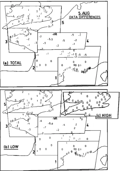
(e.g., Figure 6; August 5). On this
approximately
equal
in
both
fre-
• VT,:13
1 5 3 9 3 /9 •
3 day
the
satellite
and
surface
observers
agree
that
there
is
•-- 7
9•=..•.,•..•
'
//
little
or
no
high
cloud,
giving
rise
to
the
zeroes
in
Figure
7
• •-'1
17••..._/6
7 8 1 õ½.
The
8-okra
differences
in
the
low-cloud
retrievals
in
o
region 4 seem to coincide
with the edges
of vertically de-
• -3•
•3
1••
veloped
clouds.
The
apparent
overestimateby
the
satellite
n
-> T•, 9 9 1
• is related to the retrieval method, which does not allow for
• partial coverage of individual pixels and can thus confuse
• Ti-r"21
2•32• 25
/ /6 i
pixels
partially
covered
by
a
particular
cloud
type
with
an-
• •__•••
other
cloud
class.
• ZI.-37•43
37 21 Z.
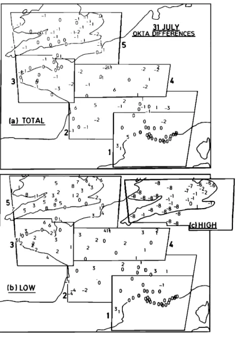
Region
5 on
July
31 (Figure
7) exhibits
the
clearest
exam-
• '•s••i•iL••
]
••/
•
Z,
9
2
azIlount8
ple
of
obscuration
can be seen
of
to be in almost
cloud
by
other
perfect agreement
layers.
The
total
cloud
(Fig-
• d •
7•k• k
are
7a)
'while
the
surface
observer
overestimates
low-cloud
/-'- 3, 3
18,60 14,,7
,x
9,[
\\k 1,3
•
9
'12
9
•aznount
(Figure 7b) and the satellite
retrieval overestimates
i
•[ rrr •
• •: v• vm
high-cloud
amount
(Figure
7•). In both
cases
the
differences
SURFACE OBSERVATIONS (OKTAS) range up to 8 oktas.
4024 HENDEI•SON-SELLE•tS ET AL.: SUB. FACE AND SATELLITE CLOUDINESS FOR EUI•OPg IN 1983 TOTAL CLOUD - 8 -6 -z, -2 0 satellite overestimate ( surface underestimate )
900
800 700 6 surface overestimate (satellite underestimate ) i i -8 -6 -z. -2 satellite overestimate ( surface underestimate -900 8OOb
700 600 5OO z, oo 2oo1
oo••.•
0 • • • • surface overestimate { satellite underestimate )Fig. 3. (a) Frequency distribution of the difference of total
cloud amount in oktu between the surface observer and satel-
lite retrieval for the 124 stations over the 20 days. (Positive
values occur when surface values are greater than satellite re-
trievalz.) (b) As for Figure 3a, except agreement in totally
clear and totally cloudy skies hu been removed from the zero-
difference column. (Positive values occur when surface values are greater than satellite retrievals.)
August 10, 1983. July 30 was one of the hottest days on record for France and is correspondingly the most cloud free
of all the 20 days in the study. Very good agreement is seen
in both the total and low-cloud amount difference maps.
There are a large number of zeroes, not just in region 1 but in regions 2 and 4 as well. On August 10 a subjective analysis of the visible and infrared photographs shows the east of
England and the Welsh borders to be covered
by low cloud
which appears to be due to a peculiarity at that particular station, the difference between the two low-cloud retrievals
is less than 2 okras.
For the stations of Wyton, Mumbles Head, Cardiff, and Exeter, detailed results are given in Table 4. The satellite retrieval includes cloud layers other than low clouds. An investigation of the retrieval for these particular stations shows that extreme edges of low clouds have sometimes been classified as higher semitransparent clouds and that some groups of pixels around coastlines, showing high variances, have been classified as partial coverage with medium clouds.
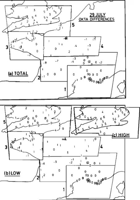
On July 28 and 29, region 5 exhibits large surface ob-
server overestimates in the total cloud amount difference
maps. On the July 29, 13 of the 32 stations show a surface
observer
overestimate
of 4 okras or more (Figure 8a). The
LOW CLOUD satellite overestimate ( surface underestimate ) 900 surface overestimate ( satellite underestimate ) ! ! 1 -8 -6 -z. -2 satellite overestimate ( surface underestimate 9OO 800
b
700 600200
100
surface overestimate( sat ellit e underestimate
or fog
but the
rest
of England
and
Wales
to be cloud
free. Fig. 4. (a) Frequency
distribution
of the
difference
of low-
On this day there was a high-pressure area stationary off cloud amount in oktu between the surface observer and satel-
the northeast coast of Britain, with a ridge extending
from lite retrieval
for the 124 stations
over the 20 days. (Positive
Scandinavia
to the Azores.
There
is no evidence
to suggest values
occur
when
surface
values
are greater
than
satellite
re-
trievals.) (b) As for Figure 4a, except agreement in totally
upper
level
cloud.
Ground
observers
and
satellite
retrievals
clear
and
totally
cloudy
skie•
has
been
removed
from
the
zero-
agree
for most
of the stations,
finding
either
clear
sky or difference
column.
(Positive
values
occur
when
surface
values
low clouds. With the exception of the 5- okra difference, are greater than satellite retrievals.)HENDERSON-SELLERS ET AL.: SURFACE AND SATELLITE CLOUDINESS FOR EUROPE IN 1983 4025
TABLE 3. Number of Occurrences of okra DifFerences* for the Types of Cloud Studied
Difference Total Observation Number of Type -8 -7 -6 -5 -4 -3 -2 -1 0 1 2 3 4 5 6 7 8 Observations Total Cloud 1 11 18 33 78 186 338 636 720 244 120 52 21 11 8 0 2 2480 (323) Low Cloud 6 6 13 21 52 õ3 103 209 818 õõ2 260 201 119 29 18 14 6 2480 (241) High Cloud 40 33 25 21 32 41 70 80 233 28 23 22 19 I 3 I 0 680 (11)
*Difference is stated in oktas.
Number in parentheses is the number of occurrences of total, low- or high-cloud differences of zero okras which were not due to clear or totally overcast conditions.
low-cloud
amount difference
maps (Figure 8b) show
surface
observer overestimates, however, they are much smaller than in the total cloud amount, typically 1 okra. Moving to the high-cloud amount difference maps, there are large surface observer overestimates, 5 okras and above on July 28 and 3okras and above
on July 29 (Figure 8c). Ignoring
zero okra
cases on July 28, the surface observer reports either 6 or 7 okras, whereas the satellite never retrieves more than 1 okra. More remarkably, on July 28, only 3 of the 32 surface ob- servers report zero okras high-cloud amount; the rest report 3 - 6 okras, with one 7-okra report. The satellite-retrieved high-cloud amount at all 32 stations is zero okras. Subjec- tive analysis of the METEOSAT visible and infrared photos suggests some low clouds covered with a tenuous layer ofcirrus.
These preliminary results indicate that when there is no cloud, the surface observer and satellite retrievals agree. On days that were cloudy, particularly when several cloud lay- ers, including cirrus, occurred, the total cloud agreement was reasonable, usually within 2 okras. In many cases, when the satellite detected a total coverage, the observer reported only 7 okras. For low cloud, however, the agreement was very poor, with the satellite underestimating by between 2 and 5 okras. This disagreement seems to be due to upper level cloud obscuring the satellite's view of the low cloud.
4. SOME POSSIBLE SOURCES OF DISCREPANCIES
The results presented above underline the basic problem inherent in all comparisons between surface and satellite observations: the upward view of the surface observer dif-
fers from the downward view of the satellite sensor. Note
how the low-cloud amount frequency
distribution (Figure
4) shows
a skew toward a satellite
underestimation
due to
the low clouds being obscured by high clouds. Similarly, thehigh-cloud
amount frequency
distribution
(Figure 5) shows
a slight skew towards a surface observer underestimation due to the high clouds being obscured by the low clouds.All the differences are not so simply resolvable. The dif-
ferences
of layer and total cloud estimates
(Figures 6, 7,
and 8) are extremely
•spotty' suggesting
a range of mecha-
nisms
causing
differences.
Also, although
Barnes
[1966]
and
Malberg
[1973]
both found that the surface
observer
tended
to overestimate the total amount of cloud compared to thesatellite, the results presented here show a tendency for the
opposite: for the satellite to overestimate total cloud amount
HIGH CLOUD
400
300
satellite surface
overestimate overestimate
(surface underestimate ) ( satellite underestimate )
4OO
b
3OO 200 lOO•
,
i
i
,
!
'1
- -6 -4 -2 0 2 4 6 8 satellite surface overestimate overestimate(surface underestimate) (satellite underestimate)
Fig. 5. (a) Frequency distribution of the difference of high-
cloud amount in okras between the surface observer and satel-
lite retrieval for the 34 British stations over the 20 days. (Posi-
tive values occur when surface values are greater than satellite
retrievals.) (b) As for Figure 5a, except agreement in totally
clear and totally cloud skies has been removed from the zero-
difference column. (Positive values occur when surface values
4026 HENDEItSON-SELLEitS ET AL.: SURFACE AND SA?gLLITE CLOUDINESS FOP,. EUROPE IN 1983
•---•_-•1.---'•
(• '-11 •'-z..
I/ OKTA
DI'--•'•ENCES
/
' , o•
]
-•
-]
-]• -10-5 -5
AL •-
00 0 0
l=
- -•
0
---
-
0
TOT
•
oo
o•
! -'
• , -71
2
o 1
(b) LOW
o
l
1 11
1_
1 0
1 o o o o oo Ol00
0
Fig. 6. (a) The difference of total cloud amount in okras between the surface observer and satellite retrieval for the 124 stations for August 5, 1983. (Positive values occur when surface values are greater than satellite retrievals.) (b) As for Figure 6a, but for low cloud. (c) As for Figure 6a, but for high cloud.
(Figures 2a and 3b). In the following
four subsections
some
possible causes of the observed discrepancies are examined.4.1. Resolution Di•erences Between Two Kinds of Measureme•s
In the satellite retrieval algorithm used here, each pixel,
representing
an area of about 50 km
2, is classified
as non-
cloudy or as covered with a particular class of cloud. For
a ground
observer,
clear and overcast
conditions
(for differ-
ent cloud types) are also easily identified
for a similar area.
This is particularly true if the area is directly above the ob- server. Observation of a directly overhead area can result in different biases, depending on the true coverage. In the caseof few small clouds
(very sparse
coverage),
the satellite
will
underestimate the coverage by detecting no cloud under a certain threshold of signal on the two radiometric channels. Conversely, over this threshold the satellite will detect a to- tal cloud coverage for the pixel, whereas the observer will report a partial coverage.Typically, in the case of low fractional coverages, the re-
suit of this resolution difference is an underestimation by
the satellite and, in the case of high fractional coverages, an overestimation by the satellite. However, this effect is some- what attenuated by the sampling area of the satellite, which contains typically in this study 15 x 19 = 285 pixels. It
remains to be seen if such large areas are also representative
of surface observations.
4.2. RepresentativeheSS of Surface Station Observations A major problem was selecting the area over which the
satellite retrievals were to be made. Clearly, it was nec-
essary to choose an area similar to that viewed by a sur-
face observer.
As discussed
above,
Barrett and Grant [1979]
identified a theoretical maximum radius of vision of a sur-
face observer as 50 km, thus suggesting an area of size 100
km by 100 km for this comparison. On the other hand,
Barnes [1966] pointed out that the optimum method for
making such an intercomparison was not obvious because of the very different areas viewed by the satellite and surface observer. Certainly, the area viewed by a surface observer isHENDERSON-SELLERS ET AL.: SURFACE AND SATELLITE CLOUDINESS FOR EUROPE IN 1983 402?
-21
•
/
J
oO__:_o,,
øoo
o
oOo,
5oO
o 3 1
o o o -1 Ooo o/oO
o oOoSa
•cIHIGH
Fig. 7. As for Figure 6, but for July 31, 1983.
determined by the height of the clouds observed, since this
determines the "celestial dome' which he views. In a het-
erogeneous cloud configuration an observer can see further in one direction than another. This problem is compounded by variations in atmospheric transmissivity and the amount
of illumination. The problems of perspective and inhomo-
geneity in area viewed led us to reconsider the choice of area
size.
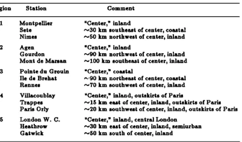
In an attempt to examine the representativeness of single- station data for an area of 100 km by 100 kin, a study of cloud reports from three surface stations in each of the five regions was undertaken. The stations concerned for each re- gion are given in Table 5. The stations were chosen for each region on the basis that they were the nearest to each other
with the most complete
set of data (i.e., avoiding
stations
for which 9 and -9 codes
had been reported). In regions
2
and 3, stations are within a 100--kin radius of each other, in regions 1 and 5 within a 50--kin radius, and in region 4 within a 20-kin radius. Note that with reference to Fig- ures 6, 7, and 8, the areas used for the satellite estimations corresponding to these stations generally have many pixelsin common: for example, 64% of the pixels for the three
stations of region 4 and 50% of the pixels for the stations
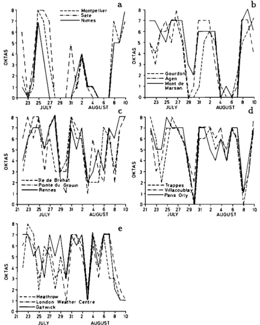
of region 5, thus reducing large differences in the satellite retrievals for these adjacent surface stations.Figures 9a - 9e are plots of 1200 UT observations for each of the three stations in the five regions for the full period. Generally, it was found, perhaps not surprisingly, that the nearer the stations were together the better the agreement; region 4 having the best overall agreement. Locational dif- ferences as well as spatial separation may cause disagree- ment. Both regions 1 and 3 contain a mixture of inland
and coastal
stations
(see Table 5) and in region
5, 50 km is
the difference between the center of London and the Sussex
countryside. Even in region 4, which has the smallest radius of station separation, differences of 2 and 3 okras can often be seen. Greater differences can be seen in other regions. For example, in region 1 on July 31, there is a discrepancy of 5 okras between Sere and the other two stations. Disagree- ment between surface observations at nearby stations can be caused by fronts moving across the region, which may result in a time lag in the increase or decrease in cloud amount be-
4028 HENDEB. SON--SELLEB. S E? AL.: SURFACE AND SATELLITE CLOUDINESS FOB. EUROPE IN 1983
TABLE 4. Satellite-- and Surface-Retrieved Low-, High-, and Total Cloud Amounts for Four Stations in l•egion 5 for August 10, 1983.
Surface Satellite Surface Satellite Surface Satellite
Station Low Low High High Total Total
Wyton 4 4 0 0 4 5
Mumbles Head 0 0 0 0 0 1 Cardiff I I 0 0 I 2 Exeter 0 0 0 0 0 I
Cloud amounts are stated in oktas.
tween
the stations
[Greenwood,
1985]. For example,
on July tion of cloud cover; the number of cases
studied
here be-
22 for the five regions, plots of all the available data showed ink too small to make significant estimations of correlationthat trends within regions were closely correlated with the coefficients as a function of the distance between stations. movement of a cold front, which passed over Paris around However, regions I and 5, with a 50-km radius around the midday. However, this type of synoptic forcing is unlikely central location, do show a reasonable consistency, which to be responsible for all the day-to-day discrepancies seen suggests that the initial choice of an area of size 100 km by in Figure 9. 100 km was satisfactory within the constraints of time and
These observations are not sufficient to identify firmly an data availability. It must be noted that the reason for the
optimal radius of representativeness of a ground observa- common 1- to 2-oktas difference between adjacent surface
HIINDE!tSON-SELLE!tS ET AL.: SURFACE AND SATELLIT• CLOUDINESS FOR EUaOP• IN 1983 4029
TABLE 5. Stations Used in Each Region to Select the Sise
of the Satellite Retrieval Area
Region Station Comment
1 Montpellier Sere Nimes 2 Agen Gourdon Mont de Marsan 3 Pointe du Grouin lie de Brehat Rennes 4 Villacoublay Trappes Paris Orly 5 London W. C. He,throw Gatwick 'Centerr inland
•30 km southeast of center, coastal ~50 km northwest of center, inland
'Center,' inland
~90 km northwest of center, inland •'•100 km southeast of center, inland 'Center,' coastal
•'90 km northeast of center, coastal •,•70 km southwest of center, inland 'Center,' inland, outskirts of Paris
~15 km east of center, inland, outskirts of Paris •,•20 km southwest of center, inland, outskirts of Paris 'Center," inland, central London
~30 km east of center, inland, semiurban •50 km south of center, inland
stations is likely to be a combination of observational un- certainty and dynamic variability in the clouds themselves. These two causes are not readily separable.
4.3. Angle o! View o! Satellite and Surface Observers
It is well known that retrieval of cloud amount from satel-
lites is subject to systematic errors whenever the viewing an-
gle •b, which the satellite subtends at the cloud, is other than
zero [e.g., Bunting
and Hardlt, 1984]. For example,
Snow
et
a/. [1985] have used photographs
from the Space Shuttle
to construct curves which show the increase in satellite-
retrieved cloud cover as a function of the viewing angle.
Cloud cover, which is 20% at a viewing angle of •b = 0 ø, increases to over 30% for •b = 50 ø.
Undoubtedly, METEOSAT is viewing the sides of cloud
at the latitudes (39 ø - 53øN) of importance
in this study.
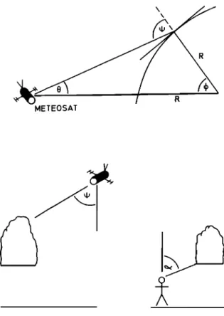
Referring to Figure 10, the angle •b, which is the satellite viewing angle from the vertical, is given by=
+
(2)
where •b is the latitude, and for METEOSAT, O is given by
0 = tan-l{
H + R cos •Rsin•
}
(3)
For a satellite height H of 36,000 km and taking the radius of the earth R = 6370 km, gives for the mean latitude of the
study area (•b = 46ø), O = 6.5 ø and hence • = 51.5
ø .
In the case of region 5 the mean latitude of the region is•b = 51ø, giving O = 7.1ø and •b = 58.1ø. Thus from
the ex•ple cited above it c• be seen that the •TEOSAT cloud retriev• is Hkely to be • overestimate, perhaps by • much • about 10 - 15• cloud •o•t.
On the other h•d, consideration is r•ely given to the fact that the s•ace obse•er •so suffers from the problem of cloud sides beco•ng importer in •s sky cover estima- tion when clouds •e either vertic•y developed or ne• to
•s horizon. The c•e of the s•ace obse•er is more &ffi-
c•t to consider, since the "e•or • in •s retriev• depen•
upon the cloud confi•ation w•ch he views (i.e., whether
the clouds •e close to the se•th or have •e•th •gles closeto 90ø). Merritt [1966] found that experienced
observers
tended to overestimate the sky cover when clouds were nearthe horizon, as compared to objective retrievals from all-sky camera photographs, but to underestimate the sky cover for clouds evenly distributed over the sky. The position of the cloud is important. A cloud overhead will look much larger
than one on the horizon as long as it is not highly verti-
cally developed
[e.g., Henderson-Sellers
eta/., 1984]. It is
possible, however, to calculate the mean viewing angle of
the observer, a, as shown in Figure 10, by assnming that
the observer
has a clear view to his horizon [HM$O, 1969]
and then integrating the viewing angle over the hemisphere,a = f•/2
/•2•.R
2 sin
I•
dl•
(4)
fo
•r/2 2•'R
2 sin • d•
On evaluation, it is found that a = 57.3 ø.
Thus excluding any considerations of atmospheric scat-
ter and absorption and assnming that a spatially homoge- neous cloud field is viewed by both the satellite and the
surface observer, it appears that at a latitude of 50.3 ø the
induced errors due to observation of cloud sides as well as the
upper or lower cloud faces are equivalent for METEOSAT and a surface observer. This latitude lies in the region stud- ied here, in fact, just north of the southern boundary of
region 5 (see Table 2).
These calculations do not, of course, demonstrate that
there will be no errors induced in the comparison between
satellite and surface retrievals of cloud amount due to the
viewing of cloud sides. However, to first order, it does seem
that the level of cloud amount overestimation will be similar for both satellite retrieval and surface observers. We there-
fore conclude tentatively that this problem is not likely to be responsible for the differences described in the preceding
sections.
4.4. Observing Practices and Bias
Another possible cause of differences between the satel- lite and the surface retrievals of cloud amount is the ability