Long-term changes and variability in a transient simulation with a chemistry-climate model employing realistic forcing

HAL Id: hal-00303900

https://hal.archives-ouvertes.fr/hal-00303900

HAL is a multi-disciplinary open access

archive for the deposit and dissemination of sci-entific research documents, whether they are pub-lished or not. The documents may come from teaching and research institutions in France or abroad, or from public or private research centers.

L’archive ouverte pluridisciplinaire HAL, est destinée au dépôt et à la diffusion de documents scientifiques de niveau recherche, publiés ou non, émanant des établissements d’enseignement et de recherche français ou étrangers, des laboratoires publics ou privés.

Long-term changes and variability in a transient

simulation with a chemistry-climate model employing

realistic forcing

M. Dameris, V. Grewe, M. Ponater, R. Deckert, V. Eyring, F. Mager, S.

Matthes, C. Schnadt, A. Stenke, B. Steil, et al.

To cite this version:

M. Dameris, V. Grewe, M. Ponater, R. Deckert, V. Eyring, et al.. Long-term changes and variability in a transient simulation with a chemistry-climate model employing realistic forcing. Atmospheric Chemistry and Physics Discussions, European Geosciences Union, 2005, 5 (2), pp.2297-2353. �hal-00303900�

ACPD

Full Screen / Esc

Print Version Interactive Discussion

EGU Atmos. Chem. Phys. Discuss., 5, 2297–2353, 2005

www.atmos-chem-phys.org/acpd/5/2297/ SRef-ID: 1680-7375/acpd/2005-5-2297 European Geosciences Union

Atmospheric Chemistry and Physics Discussions

Long-term changes and variability in a

transient simulation with a

chemistry-climate model employing

realistic forcing

M. Dameris1, V. Grewe1, M. Ponater1, R. Deckert1, V. Eyring1, F. Mager1,4,

S. Matthes1, C. Schnadt1,5, A. Stenke1, B. Steil2, C. Br ¨uhl2, and M. A. Giorgetta3

1_{Institut f ¨ur Physik der Atmosph ¨are, DLR-Oberpfaffenhofen, Wessling, Germany}

2

Max-Planck-Institut f ¨ur Chemie, Mainz, Germany

3

Max-Planck-Institut f ¨ur Meteorologie, Hamburg, Germany

4

now at: University of Cambridge, Centre for Atmospheric Science, Department of Geography, Cambridge, United Kingdom

5

now at: ETH Z ¨urich, Institut f ¨ur Atmosph ¨are und Klima, Z ¨urich, Switzerland Received: 25 January 2005 – Accepted: 3 March 2005 – Published: 14 April 2005 Correspondence to: M. Dameris (martin.dameris@dlr.de)

ACPD

Full Screen / Esc

Print Version Interactive Discussion

EGU Abstract

A transient simulation with the interactively coupled chemistry-climate model (CCM) E39/C has been carried out which covers the 40-year period between 1960 and 1999. Forcing of natural and anthropogenic origin is prescribed where the characteristics are sufficiently well known and the typical timescales are slow compared to synop-5

tic timescale so that the simulated atmospheric chemistry and climate evolves under a “slowly” varying external forcing. Based on observations, sea surface temperature (SST) and ice cover are prescribed. The increase of greenhouse gas and chlorofluro-carbon concentrations, as well as nitrogen oxide emissions is taken into account. The 11-year solar cycle is considered in the calculation of heating rates and photolysis of 10

chemical species. The three major volcanic eruptions during that time (Agung, 1963; El Chichon, 1982; Pinatubo, 1991) are considered. The quasi-biennial oscillation (QBO) is forced by linear relaxation, also known as nudging, of the equatorial zonal wind in the lower stratosphere towards observed zonal wind profiles. Beyond a reasonable repro-duction of mean parameters and long-term variability characteristics there are many 15

apparent features of episodic similarities between simulation and observation: In the years 1986 and 1988 the Antarctic ozone holes are smaller than in the other years of the respective decade. In mid-latitudes of the Southern Hemisphere ozone anomalies, especially in 1985, 1989, 1991/1992, and 1996, resemble the corresponding observa-tions. In the Northern Hemisphere, the first half of the 1990s is dynamically quiet, no 20

stratospheric warming is found for a period of at least 6 years. As observed, volcanic eruptions strongly influence dynamics and chemistry, though only for few years. Obvi-ously, planetary wave activity is strongly driven by the prescribed SST and modulated by the QBO. Preliminary evidence of realistic cause and effect relationships strongly suggest that detailed process-oriented studies will be a worthwhile endeavour.

ACPD

Full Screen / Esc

Print Version Interactive Discussion

EGU 1. Introduction

In recent years, more and more results of interactively coupled chemistry-climate models (CCMs) have become available (e.g.Rozanov et al.,2001;Austin,2002; Na-gashima et al.,2002;Pitari et al.,2002;Schnadt et al.,2002;Steil et al.,2003;Manzini et al.,2003). First of all, they have been developed to examine the feedback between 5

dynamical, physical, and chemical processes in the atmosphere, with a particular focus on the upper troposphere and stratosphere. The primary purpose of CCMs is to sup-port analyses of long-term observations and to explain recent changes and variability of the chemical composition and dynamics. Like other complex model systems, CCMs must carefully be checked with respect to their abilities and deficiencies to describe 10

present and recent atmospheric conditions before they can be applied for reliable esti-mates of future changes.

Currently, there are two concepts to perform numerical experiments with CCMs: Firstly, so-called time-slice experiments are well suited to investigate the internal vari-ability of the coupled chemistry-climate system and to indicate and estimate the sig-15

nificance of specific changes of certain parameters or processes in past, present or future climate states with respect to a reference state. Such simulations are carried out with fixed boundary conditions given for a specific year, for example, concentrations of greenhouse gases (GHGs), emissions of natural and anthropogenic source gases, sea surface temperatures (SSTs), etc., to investigate the corresponding “equilibrium 20

climate”. The comparison of time-slice simulations among each other is favourable to identify and interpret long-term temporal developments, e.g. pattern changes, in case that the assessment of statistical significance poses a problem. Secondly, transient model simulations, which involve gradual changes in GHGs and other boundary condi-tions, allow a more direct comparison with the corresponding continuous behaviour of 25

the observed atmosphere. In particular, non-persistent perturbations of the stationary or slowly varying behaviour of the real atmosphere can be included in the simulation for a more detailed model evaluation. Both strategies of model simulations lead to useful

ACPD

Full Screen / Esc

Print Version Interactive Discussion

EGU results to better understand atmospheric processes. This is demonstrated by a

con-siderable number of papers which have recently been published (e.g.Rozanov et al., 2001;Austin,2002;Nagashima et al.,2002;Pitari et al.,2002;Schnadt et al.,2002; Steil et al.,2003;Manzini et al.,2003). A number of examples of concerning strengths and weaknesses of CCMs were discussed inAustin et al.(2003) where the results of 5

different CCMs have been compared with observations and each other. The studies mentioned above have concentrated on the stratosphere, other ones have the main fo-cus on the troposphere (e.g.Wang and Prinn,1999;Johnson et al.,1999;Grewe et al., 2001a). All these CCM studies have in common that they focus on specific causes and effect relationships with respect to atmospheric chemistry and dynamics, but rarely try 10

to investigate the complete system.

It is the central objective of this paper to investigate and discuss the results of a transient simulation with a state-of-the-art CCM. While E39/C simulates tropospheric and lower stratospheric processes as components of equal importance, the focus of our analysis is on the upper troposphere and lower stratosphere. Moreover, we have tried 15

to include a comprehensive set of external forcings on variability and trends in order to allow a fair comparison with observations and to assess the capability to reproduce the development of the real atmosphere. To our knowledge, this is one of the first transient CCM simulations which, beyond trends in trace gas emissions and concentrations, also considers the observed sea surface temperature (SST) variability, the impact of large 20

volcanic eruptions, the 11-year solar cycle effect, and the quasi-biennial oscillation (QBO). They all have significant impacts on processes which determine the dynamics and chemistry of the atmosphere. The aim of this investigation is to identify and better understand the importance of external forcings on climate and chemical composition. For example, a key question is the deterministic behaviour of a non-linear model system 25

to such forcings. A detailed comparison of model results and data products derived from long-term observations is presented to advance our understanding for answering the above questions.

set-ACPD

Full Screen / Esc

Print Version Interactive Discussion

EGU up is given. Section 3 concentrates on long-term changes (trends) in observations

and model data. The variability due to prescribed forcings (i.e. volcanic eruptions, QBO, solar cycle, SSTs) are discussed in Sect. 4. The results discussed in this paper concentrate on the upper troposphere and lower stratosphere region (UTLS), which is conditioned by the model domain. The last section gives some conclusions and an 5

outlook.

2. Model description and experimental set up

2.1. The CCM ECHAM4.L39(DLR)/CHEM

In this study, the interactively coupled CCM ECHAM4.L39(DLR)/CHEM (hereafter: E39/C) is used for a transient model simulation covering the time period from 1960 10

to 1999. The model system has been applied previously for several investigations, but there results from time-slice runs were used exclusively. A basic description about E39/C is given in detail byHein et al.(2001),Grewe et al.(2001b), andSchnadt et al. (2002). In the following, the setup of E39/C is only briefly summarised.

The horizontal resolution of E39/C is T30, i.e. dynamical processes have an isotropic 15

resolution of about 670 km. The corresponding Gaussian transform latitude-longitude grid, on which the model physics, chemistry, and tracer transport are calculated, has a mash size of 3.75◦×3.75◦. In the vertical, E39/C has 39 layers from the surface up to the top layer of the model centred at 10 hPa (Land et al., 2002). The chemistry model CHEM (Steil et al.,1998) is based on a generalised improved family concept 20

which has three upgrades: 1) get rid of the general use of steady state; b)consider coupling between families by solving combined families; and c) definitions of families for transport and chemistry are different. CHEM describes relevant stratospheric and tropospheric O₃ related homogeneous chemical reactions and heterogeneous chem-istry on PSCs and sulphate aerosols, it does not include bromine chemchem-istry. The model 25

ACPD

Full Screen / Esc

Print Version Interactive Discussion

EGU reactions JPL (2000). Two heterogeneous reactions on stratospheric aerosol have

been added (ClONO₂+HCl→Cl₂+HNO₃and HOCl+HCl→Cl₂+H₂O). The transport of chlorine components has been improved by transporting both total chlorine and the partitioning of chlorine species, to minimise numerical diffusion in regions with lower vertical resolution. The net heating rates and photolysis rates in E39/C are calculated 5

using the actual three-dimensional (3-D) distributions of the radiatively active gases O₃, CH₄, N₂O, H₂O, and CFCs, and the 3-D cloud distribution. The model climatology has been extensively validated; specifically, analyses on the model’s performance in the Arctic stratosphere have been carried out (Hein et al.,2001;Austin et al.,2003).

The photolysis at solar zenith angles (SZAs) larger than 87.5◦has been implemented 10

into E39/C to account for the effects of twilight stratospheric ozone chemistry.Lamago et al. (2003) showed that the temperature, as well as ozone fields particularly in polar regions are more realistic when SZAs up to 93◦ are considered. The photolysis fre-quencies for SZA larger than 87.5◦are parameterised multiplying the photolysis rate at 87.5◦ with an exponential correction factor for SZAs up to 93◦ (for details see Lamago 15

et al., 2003).

The lightning parameterisation developed byPrice and Rind(1992), which was used in E39/C so far to account for NO_x emissions from lightning, has been replaced by an improved parameterisation developed byGrewe et al.(2001b). Grewe et al. relate the flash rate to the vertical air mass exchange within a convective cloud. A comparison of 20

flash frequencies calculated by E39/C and derived from the Optical Transient Detector (OTD) observations onboard the MicroLab satellite, showed a qualitatively and quan-titatively reasonable agreement (Kurz and Grewe,2002). The parameterisation takes into account intra-cloud and cloud to ground lightning (Price and Rind,1993) and uses effective NO_x emission profiles (Pickering et al.,1998). The annual mean emission 25

ACPD

Full Screen / Esc

Print Version Interactive Discussion

EGU 2.2. Design of the transient simulation

The transient integration of E39/C is designed to represent the development during the period from 1960 to 1999. A spin-up of ten years for stationary conditions of the late 1950s preceded the actual transient part of the experiment. The simulation aims to reproduce the effect of natural, as well as anthropogenic forcings. The natural fac-5

tors considered in the transient integration are the 11-year solar cycle, the QBO, and the chemical and direct radiative effects of the major volcanic eruptions of Agung in 1963, El Chichon in 1982, and Mt. Pinatubo in 1991. The anthropogenic influence is represented by specifying atmospheric concentrations of the most important GHGs, chlorofluorocarbons (CFCs), and nitrogen oxide emissions. However, part of the an-10

thropogenic effect is also accounted for by using an SST development prescribed from observations.

Table 1 gives an overview of the boundary conditions for the transient simulation. The SSTs are prescribed as monthly means following the global sea ice and sea sur-face temperature (HadISST1) data set provided by the UK Met Office Hadley Centre 15

(Rayner et al.,2003). These data are based on blended satellite and in situ observa-tions. A few gaps in sea ice coverage caused by interpolation to the model grid have been removed by a careful consistency check.

Both chemical and direct radiative effects of enhanced stratospheric aerosol abun-dance from large volcanic eruptions are considered. For heterogeneous reactions cov-20

ered in the chemistry module, sulphate aerosol surface area densities partly had to be approximated from observations as follows: The original data set consists of monthly and zonally averaged sulphate aerosol surface area densities (WMO, 2003). It was deduced from satellite-based extinction measurements (SAGE I, SAGE II, SAM II, and SME), as has been described in Jackman et al. (1996), using the methodology of 25

Rosenfield et al.(1997). The Agung eruption in 1963 is not covered by this data set. As a remedy, the well-documented years following the eruption of Mt. Pinatubo (1991– 1994) have been adopted and associated with the period 1963–1966 with

modifica-ACPD

Full Screen / Esc

Print Version Interactive Discussion

EGU tions based on published results to account for differences in total mass of sulphate

aerosols inside the stratosphere, in maximum height of the eruption plumes, and in the volcanoes’ geographical location (e.g.Sato et al., 1993; Andronova et al.,1999; Robock,2000). Above the maximum vertical extent of Agung’s eruption plume the an-nual mean of 1979 has been incorporated. By 1979 the total mass of stratospheric 5

sulphate aerosol had probably returned to its background value, being maintained by a permanent supply of tropospheric sulphur species (Junge et al.,1961;Mc Cormick et al., 1995). For the time periods 1960–1962 and 1968–1978 the annual mean of 1979 has been adopted, and for the period 1996–1999 the annual mean of 1995 has been used. Additionally, the data set has been interpolated linearly both from 177 to 10

16 vertical levels, and from 18 latitudes to 48 latitudes.

Eruption-related radiative heating is implemented in E39/C using pre-calculated monthly and zonally mean net heating rates. These rates were available from a previ-ous ECHAM4(T42)/L19 (L19=19 vertical layer) Pinatubo sensitivity experiment, which was forced by a realistic space-time dependent aerosol distribution (Kirchner et al., 15

1999). The original data set extends from July 1991 to April 1993. Thus, only part of the eruption-influenced time span was available, e.g. June 1991 (month of eruption) is missed. Therefore, for June 1991 the radiative forcing has been taken as 0.5×July 1991 values, and an exponential decay has been adopted in the period from May 1993 to July 1993. With regard to the Agung and El Chichon eruptions, the Pinatubo net 20

heating rates have also been used without major changes, because there were strong hints for a similar radiative heating (e.g.Labitzke, 1994). Finally, the data have been interpolated from L19 to L39 (i.e. number of vertical layers in E39/C).

The QBO is generally described by zonal wind profiles measured nearby the equator. Radiosonde data from Canton Island (1953–1967), Gan/Maledives (1967–1975) and 25

Singapore (1976–2000) have been used to develop a time series of monthly mean zonal winds at the equator (Naujokat,1986;Labitzke et al.,2002). This data set covers the lower stratosphere up to 10 hPa. It is used to assimilate the QBO in E39/C, such that the QBO is synchronised with other external inter-annual variations prescribed in

ACPD

Full Screen / Esc

Print Version Interactive Discussion

EGU this experiment. For the assimilation it is assumed that the QBO is zonally symmetric

and that it has a Gausian half width of about 12◦ latitude around the equator. The QBO is forced in E39/C by a linear relaxation of the predicted zonal wind towards the constructed QBO time series, which follows the observed zonal wind profile (Giorgetta and Bengtsson,1999). This assimilation is applied equatorwards of 20◦ latitude from 5

90 hPa up to the highest layer of the model centred at 10 hPa. The relaxation time scale has been set to 7 days within the QBO core domain. Outside of this core domain the time scale depends on latitude and pressure (Giorgetta and Bengtsson, 1999). Figure1shows the results of the assimilated monthly mean zonal winds of the E39/C run for the time period 1960 to 1999. The assimilated QBO compares well with the 10

observed phase state and the observed amplitudes of the westerlies and easterlies (Giorgetta and Bengtsson, 1999, their Fig. 1).

The influence of the 11-year solar cycle on photolysis rates is parameterised according to the intensity of the 10.7 cm radiation of the sun (data available at: http://www.drao.nrc.ca/icarus/www/daily.html). Table 2 gives the values of the extra-15

terrestrial fluxes in different spectral intervals assumed for high (i.e. these values rep-resent the year 1991) and low solar activity used at the upper boundary of E39/C. The 1991 solar maximum values are employed as reference values for the calculation of respective values for maximum solar activity of the other solar cycles which are con-sidered in the transient run, i.e. 1958, 1969, and 1980. These values are scaled with 20

the intensity of the 10.7 cm flux of the corresponding years. Photolysis rates are cal-culated in 8 spectral intervals (Landgraf and Crutzen,1998). The spectral distribution of changes in extra-terrestrial flux is based on investigations presented byLean et al. (1997). The ozone columns above the model top (i.e. centred at 10 hPa) are consid-ered by a seasonally dependent climatology which is taken from HALOE observations. 25

It must be mentioned that those climatological values are an average of 6 years only and therefore do not consider changes due to the solar cycle. The impact of solar activity changes on short-wave radiative heating rates is prescribed due to changes of the solar constant (see Table 2). Short-wave radiative heating rates are considered in

ACPD

Full Screen / Esc

Print Version Interactive Discussion

EGU two spectral intervals (Morcrette,1999;Fouquart and Bonnel,1980), respecting

contin-uum scattering, grey absorption, water vapour and uniformly mixed gases transmission functions and ozone transmission.

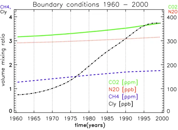
Continuously changing mixing ratios of the most relevant greenhouse gases (CO₂, N₂O, CH₄) are prescribed, CO₂for the entire model domain, the others at the Earth’s 5

surface according toHein et al. (1997) and IPCC (2001; see Fig.2). Carbon monox-ide (CO) mixing ratio is kept constant (Hein et al.,1997). Natural and anthropogenic nitrogen oxide (NO_x=NO+NO₂) emissions at the Earth’s surface, and NO_x emission from lightning and air traffic are considered. In the following a brief summary of the individual NO_xemission sources and their temporal changes is given.

10

The horizontal distribution of NO_x from industry is based onBenkovitz et al.(1996) and its temporal development has been adapted to match theIPCC(2001) values. The increase of the emission rates from 1960 to 1999 are assumed to be almost constant around 1.6%/year IPCC (1999). Anthropogenic NO_x emissions include those from surface transportation as an individual component (Matthes,2003), which contributes 15

approximately 30% to the total industry emissions (see also Matthes et al., 20051). Ship emissions have been removed from the global dataset (Benkovitz et al., 1996). Instead, a more sophisticated ship emission inventory with 1993 annual global NO_x emissions of 3.08 Tg(N) is used as the basic data set (Corbett et al.,1999). Trend es-timates of NO_x emissions from international shipping for the time period 1960 to 2000 20

have been adopted from Eyring et al. (2004)2. Based on these assumptions, the an-nual global NO_xemissions from ships for the years 1960 to 1999 amount to 1.17 Tg(N) and 3.28 Tg(N), respectively. Aircraft NO_x emissions are based on a data set repre-senting 1992 (Schmitt and Brunner,1997). Trends previous to 1992 are extrapolated

1 _{Matthes, S., Grewe, V., Sausen, R., and Roelofs, G.-J.: Global impact of road traffic}

emissions on the chemical composition of the atmosphere, Atmos. Chem. Phys. Discuss., sub-mitted, 2005.

2

Eyring, V., K ¨ohler, H. W., van Aardenne, J., and Lauer, A.: Emissions from international shipping. Part 1: The last 50 years, J. Geophys. Res., submitted, 2004.

ACPD

Full Screen / Esc

Print Version Interactive Discussion

EGU usingIPCC(1999). For the period 1992 to 1999 an exponential interpolation has been

applied. The aircraft NO_x emissions for the years 1960 to 1999 amount to 0.10 Tg(N) and 0.71 Tg(N).

Nitrogen oxide emissions from biomass burning are based onHao et al.(1990) and are revised using ASTR fire counts (David Lee, pers. comm. 2004). The trend rates 5

are roughly 0.3%/year (IPCC,1999). The global NO_xsoil emissions by micro-biological production are assumed to be constant over the four decades of the transient simula-tion. They are taken fromYienger and Levy(1995). As mentioned above, lightning NO_x emissions are calculated interactively, based on the parameterised mean mass flux in the updraft of deep convective clouds (see previous section), resulting in a mean 10

annual emission of 5.16 Tg(N). The interannual variability ranges between 4.81 and 5.42 Tg(N)/a and the seasonal cycle varies with ±14%. We anticipate that no system-atic trend of lightning NO_xemissions is found over the 40-year transient simulation.

To take into account exchange processes from the upper stratosphere, upper boundary conditions are adopted for the two families ClX and NO_y 15

at 10 hPa (ClX=HCl+ClONO₂+ClO_x, ClO_x=Cl+ClO+ClOH+2·Cl₂O₂+2·Cl₂, NO_y=NO_x+N+NO₃+2·N₂O₅+HNO₄+HNO₃). They largely determine lower strato-spheric nitrogen oxide and chlorine concentrations. Monthly mean concentrations are taken from results of the two-dimensional (2-D) middle atmosphere model of Br ¨uhl and Crutzen(1993), which also considers the effects of the 11-year solar cycle. 20

For example, the NO_y values prescribed at the model’s upper boundary fluctuate according to solar activity. Additionally, since CFCs are not explicitly transported by E39/C, they are included based on results derived from the 2-D model (depending on latitude and altitude), and serve as a source for total chlorine (Cl_y) by photolysis, within the model domain.

25

The development of CFC concentrations is prescribed in agreement with most re-cent assumptions (WMO,2003). Stratospheric Cl_y has been calculated as sum of the simulated ClO_x, ClONO₂, HCl fields, and chlorine from the prescribed CFC fields (see Fig. 2). Its temporal evolution reflects the observed development (WMO, 2003, their

ACPD

Full Screen / Esc

Print Version Interactive Discussion

EGU Figs. 1–7).

3. Long-term trends

In this section climatic variability and trends of key parameters will be presented and discussed with respect to corresponding observations.

3.1. Ozone 5

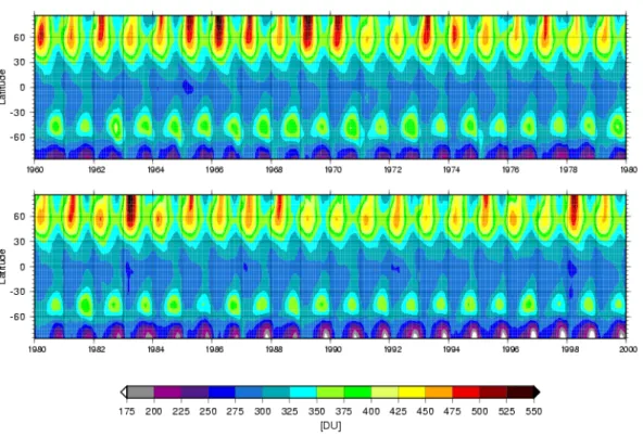
Figure3shows the development of monthly and zonal mean total ozone for the whole simulation period. It indicates the well-known features, e.g. highest ozone values in northern spring time which is highly variable from year-to-year, low ozone values in the tropics with a small seasonal cycle and little interannual variability, a relative ozone maximum in mid-latitudes of the Southern Hemisphere in late winter/early spring, and 10

a minimum ozone column above the south polar region. The ozone hole appears for the first time in the year 1982 in E39/C, which is in agreement with observations (Chubachi,1985;Farman et al.,1985). Another interesting feature is the absence of total ozone values above 475 DU in the Northern Hemisphere during the late 1980s and the first half of the 1990s. This indicates a period of at least six years without distinct 15

mid-winter warmings of the stratosphere. There is no other comparable episode in the 40-year simulation. This agrees with the evolution of the real atmosphere, where northern winters from 1989/1990 to 1996/1997 show no major stratospheric warming events (e.g.Naujokat and Pawson,1996;Naujokat et al.,1997;Pawson and Naujokat, 1999) resulting in significant springtime ozone losses during these years (e.g. Rex 20

et al.,2004).

In order to get a closer insight into regional and temporal patterns in the interannual variability of ozone changes, Fig.4shows total ozone anomalies for the whole model simulation with respect to mean values based on the years 1964 to 1980. The fea-tures discussed above can easily be identified again, especially that ozone depletion 25

ACPD

Full Screen / Esc

Print Version Interactive Discussion

EGU starts first in high latitudes of the Southern Hemisphere and that the reduction of the

ozone layer occurs later in the Northern Hemisphere and the tropical region. But there are also some additional eye-catching features: For example, as identified in observa-tions (e.g.Bojkov and Fioletov,1995), the ozone holes in the years 1986 and 1988 are clearly smaller than in the respective year before. A closer inspection of the dynamics 5

of the polar vortices in E39/C during these years indicate in both cases that the vortex is less stable and displaced from the polar region towards lower latitudes, which is very similar to the observed dynamical behaviour of the polar vortices in 1986 and 1988. There are a number of other interesting similarities in mid-latitudes of the Southern Hemisphere, i.e. modelled positive and negative ozone anomalies which nicely match 10

observations, in particular in 1985, 1989, 1991, 1992, and 1996 (see Bojkov and Fi-oletov, 1995, their Plate 1). A process related discussion about possible reasons for these consistencies with observations will be given in the next section. Looking into the tropics, there is distinct variability clearly reflecting the QBO signal; this is discussed in more detail in Sect. 4.2.

15

Before looking more closely at the long-term variability and changes (trends) cal-culated by the model, we take a look at the systematic bias of total ozone in E39/C. Figures5a and5b show 20-year mean climatological total ozone values derived from the E39/C simulation, i.e. the 1960s and 1970s, and the 1980s and 1990s. The clima-tology derived from measurements of the TOMS instrument for the years 1980 to 1999 20

is displayed in Fig.5c. A comparison of Figs.5b and 5c indicates that E39/C is able to reproduce the main features (e.g. regional distribution, seasonal cycle) in qualita-tive agreement with TOMS observations. In the Northern Hemisphere and the tropics, the model calculates total ozone values which are about 10 to 15% higher than those values derived from TOMS. These model results confirm the findings of the E39/C time-25

slice experiments (e.g.Hein et al.,2001). However, in the Southern Hemisphere the model shows an improved behaviour with respect to former studies with E39/C: The absolute total ozone values are in overall agreement with TOMS, merely the ozone hole season in E39/C lasts slightly longer and the mid-latitude ozone maximum is somewhat

ACPD

Full Screen / Esc

Print Version Interactive Discussion

EGU higher. This model improvement can partly be attributed to the fact that large SZAs are

now considered for the calculation of photolysis rates which has a clear impact on the model behaviour, in particular in the Southern Hemisphere (Lamago et al.,2003).

Figure 5d displays the simulated differences between the two E39/C climatologies affected by the ozone hole (1980–1999; Fig.5b) and the preceding era (1960–1979; 5

Fig.5a). Since the 1960s and 1970s represent a climatological mean state of an almost unperturbed episode, this climatology can be taken as a basis to derive trends from 1980 onwards. As anticipated, largest changes are found in the south polar region during spring time, where 60 DU less ozone is calculated in the second half of the transient simulation compared with the first half. This amounts to an ozone reduction 10

of about 20% per decade. Especially in the 1990s, ozone decreases steadily with more than 40% less ozone at the end of the century compared to 1980. These estimates agree well with numbers derived from observations. For example, based on TOMS-data for the years between 1978 and 1994, Mc Peters et al. (1996) estimated the ozone loss to be 20%/decade.

15

Also in the Northern Hemisphere, the trend pattern and absolute numbers agree with analyses from measurements: McPeters et al. found an ozone reduction in northern spring of about 6%/decade. The model shows a decrease of about 25 DU (Fig.5d), which relates to a trend of about 5% per decade. A small increase (i.e. less than 7 DU) in total ozone is simulated by E39/C in northern summer. It is caused by an increase 20

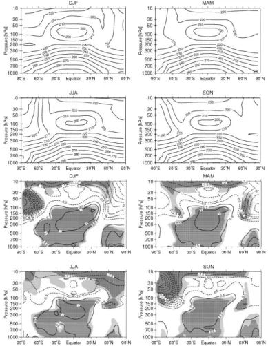
of tropospheric ozone concentration whereas at the same time no clear change is sim-ulated in the lower stratosphere (see Fig.6b). The vertical ozone distribution (Fig.6a) and its seasonal changes are very similar with results derived from E39/C time-slice experiments (e.g.Hein et al.,2001) which are in reasonable agreement with observa-tions (e.g. Fortuin and Kelder, 1998). The simulated ozone changes throughout the 25

four decades are almost everywhere statistically significant: Ozone mixing ratios have increased during equinox (MAM, SON) in the middle troposphere of the Northern Hemi-sphere by more than 10 ppbv, whereas in the lower stratoHemi-sphere a general decrease is evident, in particular in the polar Southern Hemisphere spring time (SON). The

in-ACPD

Full Screen / Esc

Print Version Interactive Discussion

EGU crease of tropospheric ozone mixing ratios are due to the increased NO_x emissions

(e.g.Grewe et al., 2001b) whereas stratospheric ozone depletion is a consequence of increased halogen loading and temperature decrease in the stratosphere due to an increased abundance of GHGs (e.g.Schnadt et al.,2002).

3.2. Temperature and zonal wind 5

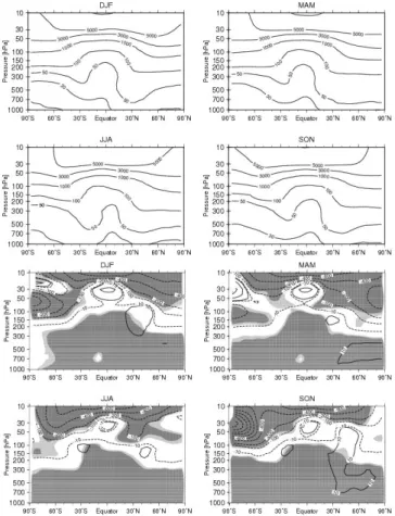
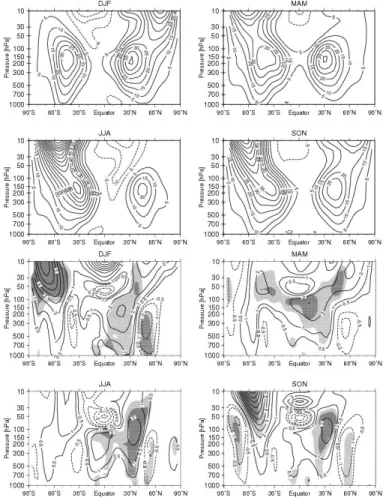
Climatologies of temperature and zonal mean wind fields for the 1960s and their changes throughout the four decades, as simulated by E39/C, are displayed in Figs.7 and8. The mean fields for the 1960s (Figs. 7a and 8a) are satisfactorily reproduced compared with NCEP re-analysis data (not shown) as well as climatological mean val-ues for the 1990s (see also Pawson et al., 2000). Sub-tropical and polar night jets 10

are clearly distinguishable, i.e. a transition zone with reduced wind speed is found in both hemispheres for all seasons. A continuous model problem arises in the Southern Hemisphere winter and spring months, where E39/C is calculating too low tempera-tures in the entire polar lower stratosphere. Therefore, the climatological mean polar vortex is too strong and stable (Fig.8a, see also Hein et al., 2001; Austin et al., 2003). 15

Another discrepancy has been identified in the zonal mean stratospheric wind fields in the summer hemispheres. The summer vortices in both hemispheres are slightly shifted towards the tropics, a wind reversal in upper model layers at higher latitudes is missed. No easterlies winds are simulated poleward of 55◦S in the Southern Hemi-sphere (DJF) and in the Northern HemiHemi-sphere (JJA), the calculated easterlies at polar 20

latitudes are too weak. The structure of temperature changes between the 1960s and 1990s (i.e. increase of tropospheric temperature, decrease of stratospheric temper-ature) partly arises from the increase in greenhouse gas concentrations, in the polar lower stratosphere it mostly reflects the decrease of ozone (Fig.7b). Strongest temper-ature decrease is seen in the Southern Hemisphere polar lower stratosphere in SON 25

(up to −10 K at 30 hPa) and DJF (up to −6 K at around 70 hPa), the time during and after the appearance of the ozone hole, which is in good agreement with assessments derived from observations (e.g.Randel and Wu,1999). A statistically significant

tem-ACPD

Full Screen / Esc

Print Version Interactive Discussion

EGU perature increase of more than 1 K is found in the (sub-)tropical upper troposphere

whereas a (non significant) cooling is calculated in the lower tropical stratosphere. The latter finding is in qualitative agreement with analyses of observations which also indi-cate a cooling trend with numbers ranging from −0.3 to −1.4 K per decade (e.g.WMO, 1999). The picture is rather unclear in the tropical tropopause region. For exam-5

ple, temperature trends derived from observations estimated at 100 hPa (WMO,1999) range from+0.3 to −0.5 K. Certainly, this is a difficult region to obtain a clear trend signal, because it is the transition layer with a warming below and a cooling above. As many other models, E39/C simulates a warming in the upper troposphere, which maximises at 250 hPa, but this is not in agreement with radiosonde temperature data 10

which indicate a cooling (e.g.Parker et al.,1997). Long-term temperature changes at middle and higher latitudes of the Northern Hemisphere middle troposphere (500 hPa) derived from E39/C (Fig.7b) varies between +0.5 K (JJA) and +1.0 K (DJF), which is less than detected at the Meteorological Observatory Hohenpeissenberg, station of the German Weather Service (MOHp; 47.8◦N, 11◦E) where an increase of+0.7±0.3 K 15

per decade has been found since 1967 (Steinbrecht et al.,1998). In general, the long-term temperature changes derived from the E39/C transient model simulation confirm recent estimates from E39/C time-slice experiments (i.e. 1980 and 1990 conditions) presented also inShine et al.(2003).

Corresponding changes of the zonal mean wind field are shown in Fig. 8b. The 20

statistically significant increase of the zonal mean wind speed of up to 6 m/s in the Southern Hemisphere lower stratosphere during spring (SON) and summer months (DJF) reflect the ozone hole formation and the corresponding decrease of polar strato-spheric temperatures. Another systematic change pattern which is obvious throughout all seasons, is found in mid-latitudes of the Northern Hemisphere (the pattern is obvi-25

ous though less distinct in the Southern Hemisphere, as well). Here, the temperature change in the upper troposphere/lower stratosphere intensifies the zonal wind due to the thermal wind equation. This results in a more intense tropospheric jet stream in DJF and MAM, and tends to shift the jet stream to lower latitudes in JJA and SON. This

ACPD

Full Screen / Esc

Print Version Interactive Discussion

EGU is accompanied by a warming of the Arctic lower troposphere and a reduction of the

horizontal temperature gradient at lower altitudes, resulting in a reduction of the zonal mean wind at around 50◦to 60◦N.

To display dynamical changes of the polar vortices during the 40 model years, an analysis of zonal mean temperature and zonal wind is presented in the style of the 5

NCEP analyses (see NCEP web-page: http://code916.gsfc.nasa.gov/Data-services/ met/). Figure 9 shows climatological mean curves of the annual cycle of the zonal wind at 60◦N and S at 30 hPa (Figs. 9a and 9c) and of the zonal mean temperature at 80◦N and S at 30 hPa (Figs.9b and 9d). The different lines represent mean values for the four decades covered by the transient simulation, the shaded area denotes the 10

minimum and maximum values reached during the 1960s of the model. Similar to the results presented inHein et al.(2001), the model again shows its ability to reproduce hemispheric differences of dynamical variability changes. While the annual cycle is well captured in both hemispheres, and the mean values in the Northern Hemisphere agree well with respective analyses derived from observations, the model has again deficien-15

cies in the Southern Hemisphere, which are related to the cold bias (see discussion above). With regards to the dynamical variability of the Northern Hemisphere during winter and spring, E39/C shows reduced interannual variability in early winter. Never-theless, E39/C is able to reproduce stratospheric warmings in mid and late winter, but the number of major events is smaller than observed. In the Northern Hemisphere the 20

climatological mean values for the four decades do not indicate systematic changes (mainly due to the high dynamical variability), which is supported by analyses of ob-servations (e.g.Labitzke and Naujokat,2000). In the Southern Hemisphere the lower stratosphere do steadily change to more stable polar vortices and colder conditions in late winter and early spring. The lifetime (persistence) of the polar vortex has been pro-25

longed by about three weeks, as the comparison of the results of the 1960s with those of the 1990s shows. This is in good agreement with an estimate presented byZhou et al. (2000) who carried out their analysis on 19 years (1979–1998) of NCEP/NCAR reanalysis data and found that the Southern Hemisphere polar vortex has lasted about

ACPD

Full Screen / Esc

Print Version Interactive Discussion

EGU two weeks longer in the 1990s than in the early 1980s.

3.3. Tropopause and water vapour

Lower stratospheric water vapour trends may give a substantial contribution to the total radiative forcing of trace gas changes in the recent past (e.g. Rosenlof et al.,2001; Forster and Shine,2002). However, time series analysis results from the few available 5

observed data (e.g.Oltmans et al.,2000;Rosenlof et al.,2001;Randel et al.,2004) of stratospheric water vapour do not produce a uniform picture of the magnitude and even the sign of a respective trend. A possible feedback chain driving stratospheric water vapour trends involves trends in tropopause height (e.g.Steinbrecht et al.,2001; San-ter et al.,2003) and related tropopause temperature, which at least in the tropics may 10

control changes in the water vapour penetration from the troposphere into the strato-sphere (Zhou et al.,2001). While in the present paper we will not investigate in detail the mechanisms responsible for long-term changes of water vapour concentrations in the lower stratosphere (a paper on this individual subject will be prepared later), we will give a brief overview of the overall trend simulated in the transient simulation.

15

The changes of the thermal tropopause pressure are given in Fig.10a. Whereas no obvious systematic changes (trends) are seen in the first two decades of the simula-tion, model results indicate a gradual change in tropopause height after about 1980. In both hemispheres, E39/C simulates a decrease (increase) of tropopause pressure (height) poleward of around 50◦. The subtropical regions show an increase (decrease) 20

of tropopause pressure (height). There appears to be no uniform trend throughout the 40-year simulation in the tropics. The major volcanic eruptions included in the transient simulation lead to a temporary increase of tropopause pressure. Changes in tropopause temperature (not shown) are directly related to the variability of the tropopause height: An increase (decrease) of tropopause height goes along with a 25

decrease (increase) of tropopause temperature. A comparison with an analysis of tropopause height changes at MOHp, 47.8◦N (Steinbrecht et al., 1998; 2001) shows a qualitative agreement, i.e. a more or less steady increase of tropopause height in

ACPD

Full Screen / Esc

Print Version Interactive Discussion

EGU February during the last 30 years. However, the model underestimates the rise in

tropopause height compared to the estimates by Steinbrecht et al. (2001). Whereas Steinbrecht et al. finds an increase of+125 m/decade for the station MOHp, E39/C cal-culates only about+80 m/decade for the corresponding model grid point. A possible explanation for the rise of tropopause height could be the warming of the troposphere 5

and the accompanying cooling of the stratosphere (Steinbrecht et al., 2001). If this would be the case, the difference between model results and observations can be ex-plained by the fact, that tropospheric warming in the model at Northern Hemisphere mid-latitudes is smaller than observed (see discussion above).

Figure 10b depicts the changes of water vapour mixing ratio at the thermal 10

tropopause during the 40 year model simulation. An uniform trend is obvious only in the subtropical region, where water vapour mixing ratios are higher in the late 1980s and the 1990s. Long-term changes are not uniform in the tropics, and neither at middle and high latitudes of both hemispheres. As discussed before, the volcanic eruptions involve characteristic signatures (see also below).

15

The general distribution of the change pattern in the lower stratosphere is equal to that at the tropopause. E39/C results, which allow a comparison with measurements of the Boulder frost point hygrometer and corresponding HALOE data discussed in Randel et al.(2004) (their Fig. 8a), are presented in Fig.11for the lower stratosphere (80 hPa). The figure shows not only the results at 40◦N, but also at 40◦S, since the 20

temporal development is very similar.

A comparison between the measurement time series of stratospheric water vapour over Boulder (Oltmans et al.,2000) and the respective model data for the period after 1979 indicates a systematic model error with respect to the absolute concentration but good agreement with respect to the observed trend during these two decades (Stenke 25

and Grewe,2004). While the simulated stratospheric water vapour distribution could be significantly improved by including methane oxidation (e.g.Hein et al.,2001), it has also been established that the Boulder trend, as well as other observed trends during the 1990s are too strong to be explained by methane oxidation alone (Rosenlof,2002).

ACPD

Full Screen / Esc

Print Version Interactive Discussion

EGU RecentlyJoshi and Shine(2003) have been proposed that part of the observed

long-term water vapour trend may be explained by the observed series of volcanic eruptions, provided that the stratospheric residence time of water vapour is in the order of 5 to 10 years and, thus, considerably longer than the residence time of the volcanic aerosols. Our model simulations do not reproduce this behaviour, as they indicate a memory of 5

little more than 4 years at about 25 km height (Fig.11).

Interestingly, E39/C simulates no positive trend in lower stratospheric water vapour mixing ratios in the years before 1980. On the contrary, a negative trend is found in the 1960s. A further discussion about possible reasons for this model behaviour is given in Sect. 4.3. Compared with the Boulder measurements one must conclude that the 10

water vapour signals of the large volcanic eruptions are overestimated in E39/C (see discussion in Sect. 4.1). In addition, a more detailed analysis of stratospheric water vapour variability and trends involving further sensitivity studies with the model system is given inStenke and Grewe(2004).

4. Variability due to external forcings

15

In this section, the model response to prescribed forcings is investigated. A guiding question for the discussion is, how deterministic the response of the non-linear at-mospheric (model) system is. We consider both abrupt perturbations (e.g. volcanic eruptions) and quasi-periodic forcings like the QBO, the 10 to 12 year solar activity cycle, and fluctuating SSTs. This is important for a better understanding of the climate 20

system to identify and quantify key parameters, which are most relevant for the descrip-tion of atmospheric variability and changes and which, therefore, must form the focus of assessments of future atmospheric changes.

ACPD

Full Screen / Esc

Print Version Interactive Discussion

EGU 4.1. Volcanic eruptions

Major volcanic eruptions strongly disturb the atmosphere, as many analyses of ob-served physical, dynamical, and chemical parameters have shown (e.g.Coffey,1996; Angell,1997a,b;Andronova et al.,1999;Robock,2000). Due to the upgraded obser-vation techniques, the documentation of effects after the eruption of Mt. Pinatubo in 5

1991 is the most comprehensive. As described in Sect. 2, the transient simulation per-formed with E39/C considers the effects of volcanoes in the chemistry, as well as in the radiation scheme of the interactive model system.

Figure 12shows a comparison of global mean temperature anomalies in the lower stratosphere derived from MSU Channel 4 (1979–2002) and equivalent temperatures 10

(derived according toSanter et al.,1999) from the E39/C transient simulation (1960– 1999). The most obvious features are the temperature increases immediately after the eruptions of Agung, El Chichon, and Mt. Pinatubo, which reach about 2 K in the simulation. The main part of the model signal originates from tropical latitudes, where maxima in the zonal mean response of more than 3 K occurs (not shown). Compared 15

to the observed lower stratosphere temperature response following the eruptions of Agung, El Chichon and Mt. Pinatubo it is evident that the model response is overesti-mated by about 1 K (see alsoWMO,1986). Kirchner et al.(1999) find a 2 K excess of their simulated temperature response (near the equator at 70 hPa, see their Fig. 5b) over observations, which they completely explain, by equal respective contributions of 20

about 1 K, from the missing QBO modulation of heating rates and missing ozone de-pletion in their model configuration. As the QBO has been nudged into our transient experiment (see Sects. 2.2 and 4.2), no inconsistency to observations occurs in this respect. Likewise, the 1 K cooling effect that observed tropical ozone depletion forces on tropical temperatures according toKirchner et al.(1999), should be included in our 25

simulation in case that the interactive chemistry-climate coupling produces the correct signal. A reduction of tropical ozone similar to the observed one is indeed evident in the simulation (Fig. 4, compare with Bojkov and Fioletov (1995)). We can not

con-ACPD

Full Screen / Esc

Print Version Interactive Discussion

EGU vincingly explain the apparent inconsistency between the conclusions ofKirchner et al.

(1999) and our results, but some possibilities are conceivable: The vertical distribu-tion of column ozone depledistribu-tion may be different in both model systems, either due to shortcomings of the chemistry-climate model or because the diagnostic method used byKirchner et al.(1999) was too simple. Similar differences may exist with respect to 5

the QBO induced heating rates. A further possibility is the different water vapour feed-back to be expected in both simulations: As the volcano-related heating of the tropical tropopause region is higher than observed in both simulations, but more distinct in the Kirchner et al. configuration, stratospheric water vapour uptake and its related radiative cooling feedback can be expected to be stronger in the simulations ofKirchner et al. 10

(1999). If this is correct, the aerosol absorption heating rates calculated by Kirchner et al. (1999) for the Mt. Pinatubo eruption and adopted in our simulations may over-estimate the actual effect after all, as they are able to balance an exaggerated water vapour radiative cooling in the original framework, but will overdo with respect to the smaller and more realistic water vapour feedback in the CCM simulation. A more spec-15

ulative reason for the overestimation of the volcano signal is the possibility of injection of moist air masses from the volcano exhaust into the stratosphere that would not be modulated by freeze drying at the tropopause. If such contribution were substantial, a mechanism of moistening and cooling the stratosphere would be absent from both the simulations ofKirchner et al.(1999) and ours.

20

The heating of the stratosphere caused by volcanic aerosol results not only in an increase of the stratospheric mean temperature of about 2 K, it also enhances the meridional circulation. The vertical ascent in the tropics is amplified by roughly 20%, which results in an uplift of the ozone profile, i.e. a vertical displacement of the ozone maximum, and a decrease of the total ozone column of approximately 5% (Stenke 25

and Grewe (2004); see also Fig.4). The additional water vapour in the tropical lower-most stratosphere is significantly enhanced, which leads to an increase of OH by 20 to 25% at 70 hPa and a significantly stronger HO_x destruction cycle. However, chem-ical timescales in the lower stratosphere are still too large compared to the dynamchem-ical

ACPD

Full Screen / Esc

Print Version Interactive Discussion

EGU timescale so that the chemical changes have only an impact on ozone in the order of

0.1% on the total column (Stenke and Grewe,2004).

In northern mid-latitudes (40◦N–50◦N) at about 50 hPa ozone concentrations are not only dynamically controlled, but also by chemistry. Relative changes of ozone produc-tion and destrucproduc-tion cycles are similar during the three volcanic episodes, except for 5

chlorine. Ozone production is reduced by 30% (Fig.13a), which is strongly determined by heterogeneous conversion (on aerosol) from N₂O₅ to HNO₃ and by the reaction NO+HO₂ followed by photolysis of NO₂ in those regions in spring. Ozone loss rates show a more complex situation. The increase in water vapour leads to a more pro-nounced HO_x destruction in the order of 50% to 100% (not shown). The NO_x cycle is 10

reduced by 20 to 40% due to a shift within the NO_ycomponents, which results from the reaction NO₂+OH→HNO₃. Ozone destruction by chlorine is doubled during the El Chi-chon period and even enhanced by a factor of 10 during the Pinatubo period compared to the non-volcanic period 1967 to 1979. In total, the enhanced ozone depletion by the HO_xcycle dominates during the Agung episode. During El Chichon, both the HO_xand 15

ClO_x cycle are of equal importance. During the Pinatubo episode the changes in the destruction cycles are clearly dominated by the ClO_xcycle. This leads to an increased ozone destruction of around 20%, 40%, and 80% during the three volcanic episodes of Agung, El Chichon, and Mt. Pinatubo, respectively (Fig.13a).

Using these changes in the production and loss rates, the effect on ozone is a re-20

duction in the order of 5% per month at 50 hPa in the period March to May, based on a simple calculation applying the ozone production and loss terms from the climate-chemistry simulation. This leads to approximately 15% ozone loss at 50 hPa during spring related to the Pinatubo perturbation, which can be revealed by comparing early winter (November) and late spring (April) ozone values at 50 hPa (Fig. 13b). Both 25

the November ozone values and the difference to the April ozone values are strongly perturbed during the post El Chichon and post Pinatubo period. Taking into account that 40% of the ozone column is affected by this process, then this reduces the ozone column by roughly 6%, which agrees with observational data (WMO,2003).

ACPD

Full Screen / Esc

Print Version Interactive Discussion

EGU The perturbation of dynamical and chemical values and parameters discussed so

far lasted only for a relatively short time period of between 1.5 and 4 years. In addi-tion, Fig.12indicates that the modelled temperature trend is in good agreement with the MSU analysis. Interestingly, similar to the changes derived from MSU data, the model results also indicate stepwise changes towards lower temperatures in the lower 5

stratosphere after the eruptions of El Chichon and Mt. Pinatubo, which is not simulated after the eruption of Agung. No temperature trend is detected in the years after El Chichon and Pinatubo, neither in MSU analysis nor in E39/C data (see alsoPawson and Naujokat,1997). Dedicated additional simulations would be necessary for a con-clusive interpretation, but a plausible explanation could be the following: The eruption 10

of Agung happened during low solar activity whereas El Chichon and Mt. Pinatubo erupted shortly after and during solar maximum, respectively. The solar cycle effect probably masks the anticipated, more or less linear negative temperature trend, which is caused by enhanced concentrations of GHGs. Slightly enhanced (reduced) temper-atures are expected in the lower stratosphere during higher (lower) solar activity due 15

to higher (lower) short-wave heating rates (e.g.Matthes et al.,2004). The calculated temperature differences (i.e. annual, global mean) between solar maximum and mini-mum in the lower stratosphere (around 15 to 25 km) are approximately 0.2 K (Matthes et al.,2003), which is the same order of magnitude that is expected from the anthro-pogenic greenhouse effect. Therefore, in the years from 1985 to 1991 and after 1996 20

with increasing solar activity, the cooling of the lower stratosphere due to increasing concentrations of GHGs might be compensated such that no temperature trend is ob-vious.

4.2. The quasi-biennial oscillation

Looking more carefully at the modelled temperature anomalies (Fig.12), in particular 25

in the years between 1965 and 1982, the QBO signal can be detected, which also contributes to the overall variability. A modulation of dynamical and chemical quanti-ties caused by the prescribed QBO is also obvious in Fig.4 in the equatorial region.

ACPD

Full Screen / Esc

Print Version Interactive Discussion

EGU Qualitatively, the QBO signal is in good agreement with a similar analysis derived from

merged satellite and ground based data (Bojkov and Fioletov, 1995; updated version until the year 2000 is at our disposal, Fioletov, pers. communication). The anomalies derived from observations and the model results are of the same order of magnitude until the 1980s (i.e. up to 6%). They are notably smaller during the 1990s in E39/C, 5

where observed fluctuations have continued with similar magnitudes. Here the mod-elled ozone varies only by about 2-3%. It seems that in E39/C the QBO signal in total ozone is partly masked by the (too) strong ozone anomalies after the volcanic erup-tions. The QBO signal in E39/C can be detected in total ozone in all latitudinal regions. For example, at mid-latitudes of the Northern Hemisphere (Fig.14), E39/C shows am-10

plitudes in total ozone of 12 DU±4 DU during winter months (JFM) which can be clearly related to the QBO. Similar results have been found in an analysis based on TOMS data (Burrows et al., 2000; see also Fig. 2.4 in EC-report, 2001). A linear regression analysis of long-term measurements of ozone at MOHp, 47.8◦N indicates QBO-related fluctua-tions of ± 10 DU (peak-to-trough ozone changes up to 20 DU) in February (Steinbrecht 15

et al.,2001). The dominant effect of the QBO in the lower stratosphere is the variation of the meridional circulation and the tropical ascent. For example, in the case of a west-erly jet (i.e. QBO east phase) the meridional circulation converges horizontally towards the jet core so that the upwelling is strongly reduced (increased) in the shear layer be-low (above) the jet. The opposite modification is found for the meridional circulation in 20

the vicinity of the easterly jet. The QBO signal in tropical upwelling explains enhanced NO_yand reduced ozone and water vapour mixing ratios, all in the range of 5% to 10% around 50 hPa. Variations of lower stratospheric ozone depletion in the tropics caused by the QBO are in the order of ±15 to 20%. Positive (negative) ozone anomalies results in enhanced (reduced) NO_x and HO_x destruction cycles. This gives a clear indication 25

that the variations of the destruction cycles are a consequence of the ozone variations and not vice versa, so that the QBO signal in column ozone is dynamically induced with some negative feedbacks from chemistry. Returning to Fig.12, quasi-biennial fluctua-tions in the global mean temperature anomalies of the lower stratosphere are visible in

ACPD

Full Screen / Esc

Print Version Interactive Discussion

EGU the E39/C data, in particular in the years between 1966 and 1982, which is a long

pe-riod without major volcanic activity. After the eruptions of El Chichon and Mt. Pinatubo a similar signature cannot be identified, neither in E39/C nor in the MSU data analysis.

4.3. The solar cycle

The impact of solar activity, in particular of the 11-year solar cycle, on climate and the 5

stratosphere has often been investigated (e.g.Haigh,1996). For example, total ozone anomalies have been estimated in the tropics (25◦N to 25◦S) for the years from 1978 to 2003 (WMO, 2003; Fig. 4-5 therein). This analysis was made on the basis of combined observations (synergistic use of ground-based and satellite data). It clearly shows strong decadal variations of total ozone in the tropics (approx. 3%), which indicates the 10

link between long-term ozone variations especially in tropical regions and the activity cycle of the sun.

Our transient simulation includes the effects of changing photolysis rates below 30 km altitude and also chemically induced ozone changes caused by prescribed time evolution of NO_y at the model top. Calculated ozone anomalies in the tropical 15

belt derived from E39/C (Fig.15) develop similarly to observations (WMO,2003), with positive anomalies around solar maximum (1981 and 1991) and negative anomalies around solar minimum (1986 and 1996). More sophisticated statistical analysis would be necessary to identify the solar cycle signal before 1978 where its presence is less but still suggested by higher ozone values around 1960 and 1969 in comparison to 20

1965. Note that the cycle between 1965 and 1976 has been less distinct, according to 10.7 cm radiation intensity records, than the other cycles included in the period. Re-calling discussions in previous sections a distinct QBO signal is immediately evident in Fig.15.

To get a better insight of the radiative impact of solar activity changes on dynamics 25

and chemistry, it is helpful to have a look at the long-term variability of ozone photol-ysis and production rates during the 40 year transient simulation. Figure 16 shows respective results of E39/C at 10, 30, and 50 hPa at lower latitudes (25◦N to 25◦S).

ACPD

Full Screen / Esc

Print Version Interactive Discussion

EGU The values calculated at 10 hPa directly reflect the prescribed changes of the

extra-terrestrial flux at the upper boundary of E39/C, which is centred at 10 hPa. The solar signal can, to some part, still be identified at 30 hPa, the picture changes further down in the lower stratosphere. At 50 hPa, the 11-year solar cycle is no longer obvious be-cause of feedback processes (e.g. interactive ozone, influence of volcanic eruptions). 5

Here, changes of ozone photolysis and production on longer time scales are identified, with minimum ozone photolysis and production rates in 1975 and higher values before and after this year. Interestingly, corresponding similar long-term changes are found in other model data sets: For example, in Sect. 3.3 it is shown that water vapour mix-ing ratios in mid-latitudes of the lower stratosphere slightly increase in the 1980s and 10

1990s, which is supported by observations at Boulder station (Oltmans et al.,2000). Model results for the 1970s indicate lowest water vapour mixing ratios without a visible trend and decreasing mixing ratios in the 1960s, whereas the values in the early 1960s are similar to those of the late 1990s. We explain these changes of water vapour mixing ratios with a corresponding behaviour of the cold-point temperature (not shown), which 15

modifies the transport of water vapour from the troposphere into the stratosphere: A decrease of the cold-point temperature is found from 1960 until the early 1970s (i.e. around 1 K) and an increase of approximately 0.5 K is calculated from the beginning 1980s to 1999. Based on the currently available model results we speculate, although we cannot definitely conclude on the basis of this analysis, that long-term changes 20

of the cold-point temperature are a consequence of solar activity fluctuations (i.e. via changes in photolysis rates, ozone production and concentration, net heating rates), although the coherence seems to be obvious.

Another parameter which has been reported to be influenced by long-term changes of solar activity is the duration of the stratospheric summer circulation at northern mid-25

and high latitudes (Offermann et al., 2004). Offermann et al. showed on the basis of meteorological analyses (e.g. NCEP, Berlin data) that the duration of summer (i.e. number of days with zonal mean east winds in 50◦ to 80◦N and 60◦ to 80◦S at 10 and 30 hPa) decreases in the 1980s and 1990s by about 10 to 20 days (depending

ACPD

Full Screen / Esc

Print Version Interactive Discussion

EGU on latitude and altitude), whereas the length of summer increases in the 1960s and

1970s with the same order of magnitude. It seems plausible that the changes found in the 1980s and 1990s may have something to do with the anthropogenic greenhouse effect and the depletion of stratospheric ozone, which both lead to a more persistent polar vortex in winter. But this explanation does not hold for the description of changes 5

found in the 1960s and 1970s. An analysis of summer duration in the E39/C transient simulation indicates a qualitatively similar behaviour as described in Offermann et al. (2004). On the basis of this result, we conclude that although solar activity is not the major driver of long-term changes of dynamical and chemical values and parameters in the lower stratosphere, it might have a stronger impact on stratospheric composition 10

and circulation as previously expected.

We are aware that the evidence of solar variability effects in the transient simulation cannot be demonstrated convincingly by the few parameters reviewed here. Probably, as experience with conventional climate models without chemistry shows (e.g. Stott et al.,2002), an ensemble of transient simulations will be necessary to establish sig-15

nificant signals. This certainly holds for studies dealing with the proposed interaction between solar cycle and QBO to modify the northern hemisphere stratospheric circu-lation (Labitzke and van Loon, 1988). However, results presented here indicate that signals in chemical parameters (like water vapour and ozone) are likely to exist. Hence it appears promising to extend our coupled CCM studies with simulations using of-20

fline chemistry (e.g.Matthes et al.,2003) to clarify the role of chemical feedbacks for dynamical changes.

4.4. Summary and discussion

It is noteworthy to which extent the temporal and spatial development of atmospheric parameters in the transient E39/C CCM simulation matches with several observed fea-25

tures. On the one hand it is not surprising that the model is able to reasonably repro-duce mean conditions and seasonal, interannual and long-term variability, since former investigations based on E39/C time-slice experiments (e.g.Hein et al.,2001;Schnadt