HAL Id: hal-00302971
https://hal.archives-ouvertes.fr/hal-00302971
Submitted on 27 Feb 2008
HAL is a multi-disciplinary open access
archive for the deposit and dissemination of
sci-entific research documents, whether they are
pub-lished or not. The documents may come from
teaching and research institutions in France or
abroad, or from public or private research centers.
L’archive ouverte pluridisciplinaire HAL, est
destinée au dépôt et à la diffusion de documents
scientifiques de niveau recherche, publiés ou non,
émanant des établissements d’enseignement et de
recherche français ou étrangers, des laboratoires
publics ou privés.
large events in the model of block structure dynamics
A. Soloviev
To cite this version:
A. Soloviev. Transformation of frequency-magnitude relation prior to large events in the model of
block structure dynamics. Nonlinear Processes in Geophysics, European Geosciences Union (EGU),
2008, 15 (1), pp.209-220. �hal-00302971�
www.nonlin-processes-geophys.net/15/209/2008/ © Author(s) 2008. This work is licensed
under a Creative Commons License.
Nonlinear Processes
in Geophysics
Transformation of frequency-magnitude relation prior to large
events in the model of block structure dynamics
A. Soloviev
International Institute of Earthquake Prediction Theory and Mathematical Geophysics, Russian Academy of Sciences, Moscow, Russia
ESP, The Abdus Salam International Centre for Theoretical Physics, Trieste, Italy
Received: 2 July 2007 – Revised: 17 September 2007 – Accepted: 21 January 2008 – Published: 27 February 2008
Abstract. The b-value change in the frequency-magnitude (FM) distribution for a synthetic earthquake catalogue ob-tained by means of the model of block structure dynamics has been studied. The catalogue is divided into time periods preceding strong earthquakes and time periods that do not precede strong earthquakes. The separate analysis of these periods shows that the b-value is smaller before strong earth-quakes. The similar phenomenon has been found also for the observed seismicity of the Southern California. The model of block structure dynamics represents a seismic region as a system of perfectly rigid blocks divided by infinitely thin plane faults. The blocks interact between themselves and with the underlying medium. The system of blocks moves as a consequence of prescribed motion of the boundary blocks and of the underlying medium. As the blocks are perfectly rigid, all deformation takes place in the fault zones and at the block base in contact with the underlying medium. Rel-ative block displacements take place along the fault zones. Block motion is defined so that the system is in a quasistatic equilibrium state. The interaction of blocks along the fault zones is viscous-elastic (“normal state”) while the ratio of the stress to the pressure remains below a certain strength level. When the critical level is exceeded in some part of a fault zone, a stress-drop (“failure”) occurs (in accordance with the dry friction model), possibly causing failure in other parts of the fault zones. These failures produce earthquakes. Immediately after the earthquake and for some time after, the affected parts of the fault zones are in a state of creep. This state differs from the normal state because of a faster growth of inelastic displacements, lasting until the stress falls below some other level. This numerical simulation gives rise a syn-thetic earthquake catalogue.
Correspondence to: A. Soloviev
1 Introduction
The study of seismicity with the statistical and phenomeno-logical analysis of observed earthquake catalogues has the disadvantage that the reliable data cover, in general, a time interval of about one hundred years or even less. This time interval is very short, in comparison with the duration of tec-tonic processes responsible of the seismic activity. Therefore the patterns of the earthquake occurrence identifiable in the catalogue may be only apparent and may not repeat in the future. This can be overcome by numerical modelling of the processes generating seismicity and analyzing obtained synthetic earthquake catalogues that cover many seismic cy-cles and allow studying the dependence of seismicity on the model parameters.
Several models based on spring-block interaction, cellular automata, scaling organization of fracture tectonics, collid-ing cascades etc. (Burridge and Knopoff, 1967; All`egre et al., 1982, 1995; Bak and Tang, 1989; Olami et al., 1992; Blanter et al., 1998; Gabrielov et al., 2000) have been de-veloped to reproduce general properties of observed seismic-ity. Other models have implemented specific mechanisms in the fault zone (e.g., Nur and Booker, 1972; Dieterich, 1972, 1994; Barenblatt, 1983; Gabrielov and Keilis-Borok, 1983; Ito and Matsuzaki, 1990; Hainzl et al., 1999; Ben-Zion and Lyakhovsky, 2006). These models reproduce certain ob-served phenomena but it is rather difficult to apply them to an actual fault system. This can be made by means of models that generate synthetic earthquake catalogues for a large het-erogeneous strike-slip fault (Ben-Zion and Rice, 1993; Z¨oller et al., 2005) and for a system of faults (e.g., Ward, 1992, 2000; Robinson and Benites, 1996, 2001; Fitzenz and Miller, 2001; Zhou, 2006).
Y
X
Lower plane
Upper plane
Dip
angle
Fault planes
Faults
Boundary blocks
a
Ribs
Vertices
Blocks
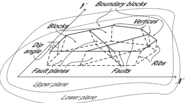
Fig. 1. On definitions used in the model of block structure
dynam-ics.
The model of the block structure dynamics (Gabrielov et al., 1990; Keilis-Borok et al., 1997; Soloviev and Ismail-Zadeh, 2003) exploits the hierarchical block structure of the lithosphere. The model is based on the assumption that blocks of the lithosphere are separated by comparatively thin, weak and less consolidated fault zones, such as lineaments and tectonic faults. In a seismotectonic process major de-formation and most earthquakes occur in such fault zones. Synthetic earthquakes are generated in the model as a result of movement of blocks creating stress in the fault zones. The model allows to reproduce the block structure of a region un-der consiun-deration and has been applied to simulate block dy-namics and seismicity of the real seismic regions (Soloviev and Ismail-Zadeh, 2003; Ismail-Zadeh et al., 2007).
A seismic region is modelled by a system of perfectly rigid blocks divided by infinitely thin plane faults. The blocks interact between themselves and with the underlying medium. The system of blocks moves as a consequence of prescribed motion of the boundary blocks and of the under-lying medium. As the blocks are perfectly rigid, all defor-mation takes place in the fault zones and at the block base in contact with the underlying medium. Relative block dis-placements take place along the fault zones. This assumption is justified by the fact that for the lithosphere the effective elastic moduli of the fault zones are significantly smaller than those within the blocks. Block motion is defined so that the system is in a quasistatic equilibrium state. The interaction of blocks along the fault zones is viscous-elastic (”normal state”) while the ratio of the stress to the pressure remains below a certain strength level. When the critical level is ex-ceeded in some part of a fault zone, a stress-drop (“failure”) occurs (in accordance with the dry friction model), possibly causing failure in other parts of the fault zones. These fail-ures produce earthquakes. Immediately after the earthquake and for some time after, the affected parts of the fault zones are in a state of creep. This state differs from the normal state because of a faster growth of inelastic displacements, lasting until the stress falls below some other level. This numerical simulation gives rise a synthetic earthquake catalogue.
The frequency-magnitude (FM) distribution (Ishimoto and Iida, 1939; Gutenberg and Richter, 1944) is described by the relation
log10N = a − bM, (1) where N is the cumulative number of earthquakes having magnitudes not less than M. The value of a in relation (1) characterises the total number of earthquakes while the value of b characterises size distribution of earthquakes. It has been shown that the value of b is not as constant and can vary in time and space. Variation of the b-value has been found for observable seismicity (e.g., Smith, 1986; Hender-son et al., 1994; Ogata and Katsura, 1993; Amelung and King, 1997; Rotwain et al., 1997; Wiemer and Wyss, 1997; Wyss et al., 2000; Wyss and Wiemer, 2000; Burroughs and Tebbens, 2002), for synthetic seismicity generated in numeri-cal models (e.g., Christensen and Olami, 1992; Narkunskaya and Shnirman, 1994; Amitrano, 2003; Zaliapin et al., 2003; Z¨oller et al., 2006) and for microfractures in laboratory sam-ples (e.g., Rotwain et al., 1997; Amitrano, 2003). Theoretical models have been developed to explain temporal fluctuations in b-value (e.g., Main et al., 1989, 1992; Henderson et al., 1992).
The purpose of the present study is to analyze the be-haviour of the b-value for the synthetic seismicity gener-ated by the model of the block structure dynamics. We try to find difference in the b-value for periods preceding the largest earthquakes and periods that do not precede such earthquakes. A simple structure consisting of 4 square blocks is used for generating the synthetic earthquake catalogue. It follows from the analysis of the synthetic catalogue that the b-value is smaller for the periods preceding the largest earthquakes. The analysis of the earthquake catalogue of the Southern California gives similar results.
2 Description of the model 2.1 Block structure geometry
A layer with thickness H , limited by two horizontal planes is considered (Fig. 1), and a block-structure is a limited and simply-connected part of this layer. Each lateral boundary of the block-structure is defined by portions of parts of planes intersecting the layer. The subdivision of the structure into blocks is performed by planes intersecting the layer. The parts of these planes which are inside the block-structure and its lateral facets are called “fault planes.”
The geometry of the block-structure is defined by the lines of intersection between the fault planes and the upper plane limiting the layer (these lines are called “faults”), and by the angles of dip of each fault plane. Three or more faults can-not have a common point on the upper plane, and a common point of two faults is called “vertex.” The direction is spec-ified for each fault and the angle of dip of the fault plane is
measured on the left of the fault. The positions of a vertex on the upper and the lower plane, limiting the layer, are con-nected by a segment (“rib”) of the line of intersection of the corresponding fault planes. The part of a fault plane between two ribs corresponding to successive vertices on the fault is called “segment.” The shape of the segment is a trapezium. The common parts of the block with the upper and lower planes are polygons, and the common part of the block with the lower plane is called “bottom.”
We assume that the block-structure is bordered by a con-fining medium, whose motion is prescribed on its continu-ous parts comprised between two ribs of the block-structure boundary. These parts of the confining medium are called “boundary blocks.”
2.2 Block movement
The movements of the boundaries of the block structure (the boundary blocks) and the medium underlying the blocks are assumed to be external force acting on the structure. The rates of these movements are considered to be horizontal and known. The movement of the underlying medium is spec-ified separately for different blocks. Dimensionless time is used in the model, and all quantities containing time are re-ferred to one unit of the dimensionless time. At each time the displacements of the blocks are determined in such a way that the structure is in a quasistatic equilibrium. All displace-ments of blocks are supposed to be infinitely small, com-pared with the block size. Therefore the geometry of the block structure does not change during the simulation and the structure does not move as a whole.
2.3 Interaction between blocks and the underlying medium The elastic force which is due to the relative displacement of the block and the underlying medium, at some point of the block bottom, is assumed to be proportional to the difference between the total relative displacement vector and the vector of slippage (inelastic displacement) at the point. This force per unit area fu= (fxu,fyu) applied to the point with
coordi-nates (X,Y ), at some time t, is defined by
fxu= Ku(x − xu− (Y − Yc)(ϕ − ϕu) − xa), (2)
fyu= Ku(y − yu+ (X − Xc)(ϕ − ϕu) − ya). (3)
where Xc, Ycare the coordinates of the geometrical centre of
the block bottom; (xu,yu) and ϕu are the translation vector
and the angle of rotation (following the general convention, the positive direction of rotation is anticlockwise), around the geometrical centre of the block bottom, for the underly-ing medium at time t; (x,y) and ϕ are the translation vector of the block and the angle of its rotation around the geomet-rical centre of its bottom at time t; (xa,ya) is the inelastic
displacement vector at the point (X,Y ) at time t .
The evolution of the inelastic displacements at the point (X,Y ) is described by the equations
dxa dt = Wuf u x, dya dt = Wuf u y. (4)
The coefficients Ku and Wu in Eqs. (2–4) may be different
for different blocks.
2.4 Interaction between the blocks along the fault planes At the time t, in some point (X,Y ) of the fault plane sepa-rating the blocks numbered i and j (the block numbered i is on the left and that numbered j is on the right of the fault) the components 1x, 1y of the relative displacement of the blocks are defined by
1x = xi− xj − (Y − Yci)ϕi+ (Y − Ycj)ϕj, (5)
1y = yi− yj+ (X − Xic)ϕi− (X − Xcj)ϕj. (6)
where Xic, Yci, Xjc, Ycj are the coordinates of the
geometri-cal centres of the block bottoms, (xi,yi), and (xj,yj) are the
translation vectors of the blocks, and ϕi, ϕj are the angles of
rotation of the blocks around the geometrical centres of their bottoms, at time t.
In accordance with the assumption that the relative block displacements take place only along the fault planes; the dis-placements along the fault plane are connected with the hor-izontal relative displacement by
1t = ex1x + ey1y, (7)
1l = 1n/cos α, where1n= ex1y − ey1x. (8)
That is the displacements along the fault plane are projected on the horizontal plane. Here 1t, 1l are the displacements
along the fault plane parallel (1t) and normal (1l) to the
fault line on the upper plane, (ex,ey) is the unit vector along
the fault line on the upper plane, α is the dip angle of the fault plane, and 1nis the horizontal displacement, normal to the
fault line on the upper plane.
The elastic force per unit area f = (ft,fl) acting along the
fault plane at the point (X,Y ) is defined by
ft = K(1t − δt), (9)
fl = K(1l− δl). (10)
Here δt, δlare inelastic displacements along the fault plane at
the point (X,Y ) at time t, parallel (δt) and normal (δl) to the
fault line on the upper plane. The evolution of the inelastic displacement at the point (X,Y ) is described by the equations
dδt
dt = Wft, dδl
dt = Wfl. (11)
The coefficients K and W in Eqs. (9–11) are, respectively, proportional to the shear modulus and inversely proportional
to the viscous coefficient of the fault zone. The values of K and W can be different for different faults.
In addition to the elastic force, there is the reaction force which is normal to the fault plane; the work done by this force is zero, because all relative movements are tangent to the fault plane. The elastic energy per unit area at the point (X,Y ) is equal to
e = (ft(1t− δt) + fl(1l− δl))/2. (12)
From Eqs. (7), (8) and (12) the horizontal component of the elastic force per unit area, normal to the fault line on the up-per plane, fncan be written as:
fn=
∂e ∂1n
= fl
cos α (13)
It follows from Eq. (13) that the total force acting at the point of the fault plane is horizontal if there is the reaction force, which is normal to the fault plane and its magnitude per unit area is equal to
p0= fltanα. (14)
We introduce the reaction force Eq. (14) and therefore there are not vertical components of forces acting on the blocks and there are not vertical displacements of blocks.
Equations (5) and (6) are valid for the boundary faults too. In this case one of the blocks separated by the fault is the boundary block. The movement of these blocks is described by their translation and rotation around the origin of coordi-nates. Therefore the coordinates of the geometrical centre of the block bottom in Eqs. (5) and (6) are zero for the boundary block. For example, if the block numbered j is a boundary block, then Xcj = Ycj=0 in Eqs. (5) and (6).
2.5 Equilibrium equations
The components of the translation vectors of the blocks and the angles of their rotation around the geometrical centres of the bottoms are found from the condition that the total force and the total moment of forces acting on each block are equal to zero. This is the condition of quasi-static equilibrium of the system and at the same time the condition of minimum energy. The forces arising from the specified movements of the underlying medium and of the boundaries of the block-structure are considered only in the equilibrium equations. In fact it is assumed that the action of all other forces (gravity, etc.) on the block-structure is balanced and does not cause displacements of the blocks.
In accordance with Eqs. (2), (3), (5–10) and (13) the de-pendence of the forces, acting on the blocks, on the trans-lation vectors of the blocks and the angles of their rotations is linear. Therefore the system of equations which describes the equilibrium is linear one and has the following form
Az = b (15)
where the components of the unknown vector z=(z1, z2, ...,
z3n) are the components of the translation vectors of the
blocks and the angles of their rotation around the geomet-rical centres of the bottoms (n is the number of blocks), i.e. z3m−2=xm, z3m−1=ym, z3m=ϕm(m is the number of the
block, m=1, 2,..., n).
The matrix A does not depend on time and its elements are defined from Eqs. (2), (3), (5–10) and (13). The moment of the forces acting on a block is calculated relative to the geometrical centre of its bottom. The expressions for the el-ements of the matrix A contain integrals over the surfaces of the fault segments and of the block bottoms. Each inte-gral is replaced by a finite sum, in accordance with the space discretization described in Sect. 2.6. The components of the vector b are defined from Eqs. (2), (3), (5–10) and (13) as well. They depend on time, explicitly, because of the move-ments of the underlying medium and of the block-structure boundaries and, implicitly, because of the inelastic displace-ments.
2.6 Scheme of simulation
Formulas given above define the stress and the evolution of the inelastic displacements at points of fault zones and of block bottoms. To carry out the numerical simulation of block structure dynamics discretization of these plane sur-faces is required. The discretization is defined by parameter
ε and applied to fault segments and block bottoms as follows.
Each fault segment is a trapezoid with bases a and b and height h=H /sinα where H is the thickness of the layer, and
α is the dip angle of the fault plane. We determine the values n1= ENTIRE (h/ε) + 1, and
n2= ENTIRE (max(a, b)/ε) + 1,
and divide the trapezoid into n1n2small trapezoids by two
groups of segments inside it; there are n1-1 segments
paral-lel to the trapezoid bases and spaced at intervals h/n1, and
n2-1 segments connecting the points spaced by intervals of
a/n2 and b/n2, respectively, on the two bases. Small
trape-zoids obtained in this way are called “cells.” The coordinates
X, Y in Eqs. (5) and (6) and the inelastic displacements δt,
δl in Eqs. (9) and (10) are supposed to be the same for all
the points of a cell and are considered average values over the cell. When introduced in Eqs. (5–10), (13), and (14), they yield the average (over the cell) of the elastic and re-action forces per unit area. The forces acting on a cell are obtained by multiplying the average forces per unit area by the area of the cell. The bottom of a block is a polygon. Prior to discretization, it is divided into trapezoids (triangles) by segments passing through its vertices and parallel to the
Y axis. The discretization of these trapezoids (triangles) is
performed in the same way as for fault segments.
The state of the block structure is considered at discrete time ti=t0+ i1t where t0is the initial time and i = 1, 2, ... .
Table 1. Notations used in the paper and values of the parameters of the model of block structure dynamics
Parameters of the model of block structure dynamics
Thickness of the layer H =20 km
Difference between the lithostatic and the hydrostatic pressure in formula (16) P =2 Kbars
Parameters for time and space discretization 1t =0.001, ε=2.5 km
Parameters of the block bottoms in Eqs. (2–4) (the same values for all blocks) Ku=1 bar/cm, Wu=0.05 cm/bars
Dip angle of a fault plane (the same value for all faults) α = 85◦
Parameters of the fault planes in Eqs. (9–11) (the same values for all faults) K=1 bar/cm, W =0.05 cm/bars, Ws=10 cm/bars
Levels of κ Eq. (16) used for the determination of earthquakes and creep (the same values for all faults) B=0.1, Hf=0.085, Hs=0.07
Parameters for determination of strong earthquakes, D- and N-periods, and b-value estimates
Magnitude cut-off that defines strong earthquakes M0
Parameters used for determination of D- and N -periods 1D, 1X
Lower magnitude threshold for b-value estimates Mt
The transition from the state at ti to the state at ti+1is made
as follows: (i) new values of the inelastic displacements xa,
ya, δt, δlare calculated from Eqs. (4) and (11); (ii) the
trans-lation vectors and the rotation angles at ti+1 are calculated
for the boundary blocks and the underlying medium; (iii) the components of b in Eq. (15) are calculated, and these equa-tions are used to define the translation vectors and the angles of rotation for the blocks.
2.7 Earthquake and creep
Earthquakes are simulated in accordance with the dry friction model. Let us introduce the quantity
κ = |f | P − p0
(16) where f=(ft,fl) is the elastic stress given by Eqs. (9) and
(10); P is assumed equal for all the faults and can be inter-preted as the difference between the lithostatic (due to grav-ity) and the hydrostatic pressure, p0, given by Eq. (14), is
the reaction force per unit area. The value of P reflects the average effective pressure in fault zones, and the difference
P −p0is the actual pressure for each cell.
Three following values of κ are assigned to each fault plane: B>Hf>Hs. If, at some time ti, the value of κ in any
cell of a fault segment reaches the level B, a failure (”earth-quake”) occurs (it is assumed that the initial conditions for the model satisfy the inequality κ<B for all cells of fault seg-ments). The failure is considered slippage during which the inelastic displacements δt and δlin this cell change abruptly
to reduce the value of κ to the level Hf. The level Hsis used
in determination of the period of the creep state as described below.
After calculating the new values of the inelastic displace-ments for all the failed cells, step (iii) of the scheme of simu-lation (Sect. 2.6) is repeated with the same values of the abso-lute displacements and rotations of the boundary blocks and the underlying medium. If after that κ>B for some cell(s) of the fault segments, the inelastic displacements are recal-culated for this cell(s), step (iii) of the scheme of simulation
is repeated and so on. When κ<B for all cells the state of the block structure at time ti+1is determined in the ordinary
way.
The cells belonging to the same fault plane, in which fail-ure occurs at the same time, form a single earthquake. The magnitude of the earthquake is calculated from
M = 0.98log10S + 3.93, (17) where S is the sum of the areas of the cells (in km2) forming
the earthquake. The constants in Eq. (17) are specified in accordance with Utsu and Seki (1954).
It is assumed that the cells in which a failure has occurred are in the creep state immediately after the earthquake. This means that the parameter Ws (Ws>W ) is used instead of W
for these cells in Eq. (11) to describe the evolution of inelastic displacements; Wsmay be different for different faults. After
each earthquake, a cell is in the creep state as long as κ>Hs,
whereas when κ< Hsthe cell returns to the normal state and
henceforth the parameter W is used in Eq. (11) for this cell.
3 Block structure under consideration and a catalogue of synthetic earthquakes
The structure under consideration and its faults on the up-per plane are shown in Fig. 2. Six faults (four of them are boundary faults) form a square with a side of 320 km divided into four smaller squares. Values of the model parameters are given in Table 1. The medium underlying all blocks of the structures does not move. The boundary movement is a translational movement at a velocity of 10 cm per unit di-mensionless time. The directions of the velocity vectors are shown in Fig. 2. The angle between the velocity vector and the proper side of the square outlining a structure is 10◦.
Numerical simulation of dynamics for the block structure under consideration was carried out for a period of 1000 di-mensionless time units starting from the initial zero condi-tion. The synthetic catalogue, which was analysed, contains earthquakes that occurred during the last 800 units of the sim-ulation. The first 200 units were not considered to exclude
1
3
4
2
a
b
Fig. 2. The structure under consideration (a) and the scheme of
its faults on the upper plane (b). The arrows show the vectors of velocities of boundaries, 1-4 are numbers of boundary sides of the structure.
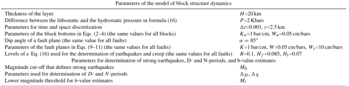
the period that is needed in the model for quasi-stabilization of the stresses after starting the simulation from the initial zero conditions. The catalogue contains 41 788 events in the magnitude interval from 4.65 to 7.58. The FM plots are given in Fig. 3. They show the number of earthquakes with magnitude M (green bars) and the number of earthquakes with magnitude not less than M brown curve (cumulative FM plot).
4 Analysis of the synthetic catalogue 4.1 Definition of D- and N -periods
We try to find difference in the behaviour of background syn-thetic seismicity during the time intervals preceding strong earthquakes (D-periods) and time intervals that do not pre-cede strong earthquakes (N -periods). Strong earthquakes are earthquakes with magnitude M>M0where M0is certain
threshold.
We consider the following definition of D- and N -periods. Let T1, T2, . . . moments of strong events (Ti+1>Ti). We use
two parameters 1D>0 and 1X≥0 and separate each interval
[Ti, Ti+1] between two consecutive strong events into three
non-intersecting intervals: D-interval, [Ti+1−1D, Ti+1);
X-interval, (Ti, Ti+1X); and N -interval, [Ti+1X, Ti+1−1D).
If Ti+1–Ti≤1D then the whole interval (Ti, Ti+1) is
con-sidered as D-interval. If 1D<Ti+1−Ti≤ 1D+1X then
the interval (Ti, Ti+1) is separated into D- and X-intervals
only without N -interval, and X-interval in this case is (Ti,
Ti+1−1D). D-period is a combination of all D-intervals
de-termined by this way and N -period is a combination of all
1 10 100 1000 10000 100000 N u m b er of ear thquak es 4 5 6 7 8 M
Fig. 3. Frequency-magnitude plots for the whole synthetic
earth-quake catalogue. Dependence of the number of earthearth-quakes on the magnitude is shown by green bars while cumulative FM plot (the number of earthquakes with magnitude not less than M) is shown by brown curve. 4 5 6 7 8 M 0.1 1 10 100 N( M ) 4 5 6 7 8 M 0.1 1 10 100 N(M )
a
b
Fig. 4. Cumulative FM plots referred to one unit of dimensionless
time constructed separately for D- and N -periods for the synthetic earthquake catalogue of the whole structure (N (M) is the number of earthquakes with magnitude not less than M): red curves concern events occurred during D-period, blue curves – during N -period.
D- and N -periods are determined with M0=7.37, 1D=1X=5 (a)
and 1D=1X=3 (b).
N -intervals. X-intervals are introduced to exclude intervals
when the background seismicity is subjected to a strong event occurred before.
The behaviour of the background synthetic seismicity is characterized using the description of the FM distribution as given in Eq. (1) for earthquakes with magnitude M<M0.
The FM distributions are obtained separately for D and N -periods. These two distributions and their description are then compared.
Table 2. Estimates of b-values of FM relations obtained separately for D- and N -periods for the whole structure, M0=7.37; uncertainty
limits of the estimated b-value are given for the confidence probability 0.95.
Parameters for determination of D- and N -periods bD(Mt) bN(Mt) bN(Mt) − bD(Mt)
Mt=5.5 1D= 1X=5 (Fig. 4a) 0.6704±0.0078 0.6854±0.0244 0.0150 1D= 1X=3 (Fig. 4b) 0.6694±0.0087 0.6731±0.0175 0.0037 Mt=6.0 1D= 1X=5 (Fig. 4a) 0.7893±0.0117 0.8951±0.0427 0.1058 1D= 1X=3 (Fig. 4b) 0.7853±0.0129 0.8416±0.0285 0.0563
4.2 Quantitative measure of the difference between FM dis-tributions
If a magnitude range M≥Mt is considered then the b-value
of FM plot in this magnitude range can be estimated as fol-lows (Aki, 1965) ˆ b(Mt) = N (Mt) ln 10 P Mi≥Mt (Mi− Mt) (18)
where N (Mt) is the number of earthquakes in the
consid-ered part of a catalogue with magnitude not less than Mt,
Mi – magnitudes of these earthquakes. Equation (18) gives
a maximum-likelihood estimate of the b-value and is used to estimate the b-values separately for D- and N -periods (bD(Mt) and bN(Mt) respectively) determined in the
cata-logue considered above. The difference between bD(Mt) and
bN(Mt) is used as a measure of the distinction between FM
distributions obtained for D- and N -periods 4.3 Analysis of the whole structure
The number of earthquakes versus the magnitude (Fig. 3) has an explicit local maximum in the magnitude range between 7.3 and 7.4. This maximum is attained at M=7.37. Accord-ingly to the definition of the magnitude in the model and geo-metrical sizes of the structure under consideration this value corresponds to an earthquake that covers completely one seg-ment of a fault plane (in the structure under consideration all segments of the fault planes have approximately the same square). This value has been preliminary taken as the magni-tude cut-off that defines strong earthquakes, i.e. M0=7.37.
Figure 4 shows cumulative FM plots constructed sepa-rately for D- and N -periods determined by using the defi-nition given above (Sect. 4.1) with 1D=1X=5 (Fig. 4a) and
1D=1X= 3 (Fig. 4b). Values of 1D and 1Xare given in
units of the dimensionless time. The number of events used for constructing the plots is referred to one unit of dimen-sionless time, i.e. the numbers of earthquakes for different magnitude ranges are divided on duration (in units of dimen-sionless time) of D- and N -periods respectively. Comparing the plots one can see difference between FM plots for D- and
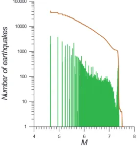
Fig. 5. Dependence of bD(6.0) (red curve) and bN(6.0) (blue curve) on M0; bD(6.0) and bN(6.0) are calculated for the synthetic earth-quake catalogue of the whole structure using Eq. (18) for D- and
N -periods respectively. D- and N -periods are determined with a
current value of M0and 1D=1X=3. Dotted curves show limits of
the confidence interval for the confidence probability 0.95.
N -periods. The plots for D-period demonstrate considerable
deficiency of events with small magnitudes in comparison with the plots for N -period. In the range of large magni-tudes (M>7.0) the incidence of the plot for N -period ob-tained with 1D=1X=5 (Fig. 4a) is appreciably greater than
that for D-period. The similar phenomenon was found for-merly for observed seismicity and in models (e.g., Narkun-skaya and Shnirman, 1994; Rotwain et al., 1997; Zaliapin et al., 2003). Results of calculation of the b-values separately for D- and N -periods (bD(Mt) and bN(Mt)) by means of
Eq. (18) with two values of Mt (5.5 and 6.0) are given in
Table 2. Uncertainty (confidence) limits of the estimated
Table 3. Estimates of b-values of FM relations obtained separately for D- and N -periods for the seismicity of the Southern California,
M0=6.4; uncertainty limits of the estimated b-value are given for the confidence probability 0.95.
Parameters for determination of D- and N -periods bD(Mt) bN(Mt) bN(Mt) − bD(Mt)
Mt=4.5
1D=1X=3 years (Fig. 9a) 1.1332±0.0569 1.4372±0.1872 0.3040
1D=1X=2 years (Fig. 9b) 1.1204±0.0615 1.3517±0.1179 0.2313
Mt=5.0
1D=1X=3 years (Fig. 9a) 1.2289±0.0933 1.5986±0.4461 0.3697
1D=1X=2 years (Fig. 9b) 1.1436±0.0929 1.5511±0.2568 0.4075
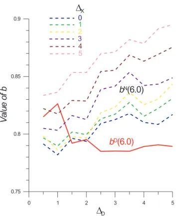
Fig. 6. Dependence of bD(6.0) (solid red curve) and bN(6.0) (dot-ted curves) on 1D and 1X; bD(6.0) and bN(6.0) are calculated
for the synthetic earthquake catalogue of the whole structure using (18) for D- and N -periods respectively. D- and N -periods are de-termined with M0=7.37 and current values of 1D and 1X. Note
that D-period and therefore bD(Mt) do not depend on 1X.
Molchan and Podgaetskaya (1973). One can see that in all cases bD(Mt)<bN(Mt) but difference bN(Mt)–bD(Mt) is
larger than the uncertainty limits of the estimated b-value only if Mt=6.0.
To check the robustness and the stability of the results with respect to parameters that determine strong earthquakes (M0)
and D- and N -periods (1D and 1X)bD(6.0) and bN(6.0)
were calculated with different values of these parameters. Figure 5 shows the dependence of bD(6.0) and bN(6.0) on
Fig. 7. Dependence of bD(6.0) (red curves) and bN(6.0) (blue curves) on M0; bD(6.0) and bN(6.0) are calculated for the
syn-thetic earthquake catalogues of the boundary fault planes 1 (a), 2 (b), 3 (c), and 4 (d) using Eq. (18) for D- and N -periods respec-tively. D- and N -periods are determined with a current value of
M0and 1D=1X=3. Dotted curves show limits of the confidence
interval for the confidence probability 0.95.
M0when 1D=1X= 3 and Fig. 6 shows their dependence on
1Dand 1Xwhen M0=7.37. Figure 6 demonstrates stability
of the result to variation of values 1Dand 1Xwhen 1D>2
but as follows from Fig. 5 the relationship bD(6.0) <bN(6.0) is valid in a narrow magnitude range about M0=7.37. The
last can be explained as follows. By definition (Sect. 2.7) the synthetic earthquakes are formed from cells belonging to the same fault plane. Behaviour of the background seismic-ity changes before a strong earthquake mainly on the same fault plane where this strong earthquake occurs. When the background seismicity of the whole structure is considered
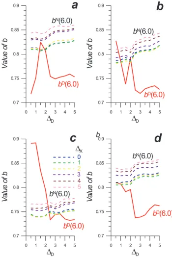
Fig. 8. Dependence of bD(6.0) (solid red curve) and bN(6.0) (dot-ted curves) on 1D and 1X; bD(6.0) and bN(6.0) are calculated
for the synthetic earthquake catalogue of the boundary fault planes 1 (a), 2 (b), 3 (c), and 4 (d) using Eq. (18) for D- and N -periods respectively. D- and N -periods are determined with M0=7.37 and
current values of 1D and 1X. Note that D-period and therefore
bD(Mt) do not depend on 1X.
periods preceding strong earthquakes for some fault planes are mixed with periods not preceding strong earthquakes for other faults and changes in the b-value before strong earth-quakes are not seen. One can avoid this by considering the fault planes separately.
4.4 Separate analysis of boundary fault planes
The strong earthquakes occur in boundary fault planes of the structure. These fault planes are marked 1–4 in Fig. 2. We considered separately catalogues of synthetic earthquakes occurred in different fault planes, and D- and N -periods were determined for each boundary fault plane accordingly to strong earthquakes occurred in it. The dependence of
bD(6.0) and bN(6.0) on M0 when 1D=1X=3 is shown
in Fig. 7 separately for different boundary fault planes.
Fig. 9. Cumulative FM plots referred to one year constructed
sepa-rately for D- and N -periods for the seismicity of the Southern Cal-ifornia, 1932–2006 (N (M) is the number of earthquakes with mag-nitude not less than M): red curves concern events occurred during
D-period, blue curves – during N -period. D- and N -periods are
de-termined with M0=6.4, 1D=1X=3 years (a) and 1D=1X=2 years
(b).
Comparing Figs. 5 and 7 one can see that for the fault planes 1 (Fig. 7a) and 2 (Fig. 7b) considered separately the magni-tude range where bD(6.0)<bN(6.0) is essentially wider than in the case of the whole structure.
Figure 8 shows the dependence of bD(6.0) and bN(6.0) on
1Dand 1Xwhen M0=7.37. One can see that if 1Dis large
enough the relationship bD(6.0)<bN(6.0) is stable with re-gard to variations of 1X. This figure does not change
princi-pally if another value of M0is selected from the range (7.20,
7.37).
5 Analyses of seismicity of the Southern California Seismicity of the Southern California has been analysed in the similar way as the synthetic seismicity obtained in the model. The data on seismicity of the Southern California have been taken from The Southern California Earthquake Data Centre (SCEDC) catalogue. It consists of hypocentral information for 1932 through the present. The information on catalogue completeness and data sources can be found at the web site (SCEDC).
Earthquakes with magnitude M≥M0=6.4 are considered
as strong events and earthquakes with 4≤M<6.4 are ana-lyzed as the background seismicity. Figure 9 shows cumula-tive FM plots referred to one year and constructed separately for D- and N -periods that were determined with 1D=1X=3
years (Fig. 9a) and 1D=1X=2 years (Fig. 9b). In the both
cases one can see difference between the plots for D and N -periods. Table 3 contains the b-values calculated separately for D- and N -periods by means of Eq. (18). As in the case of synthetic seismicity bD(Mt) is less than bN(Mt). But when
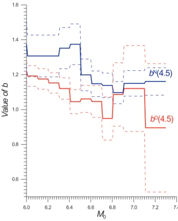
Fig. 10. Dependence of bD(4.5) (red curve) and bN(4.5) (blue curve) on M0; bD(4.5) and bN(4.5) are calculated for the
seismic-ity of the Southern California, 1932–2006 using Eq. (18) for D-and N -periods respectively. D- D-and N -periods are determined with a current value of M0and 1D=1X=2 years. Dotted curves show
limits of the confidence interval for the confidence probability 0.95.
less than the uncertainty limits of the estimated b-value, and so, Mt=4.5 has been used in the further analysis.
The dependence of bD(4.5) and bN(4.5) on the values of parameter M0, 1D, and 1X is shown in Figs. 10 and 11.
Figure 10 shows the dependence of bD(4.5) and bN(4.5) on
M0 when 1D=1X=2 years. One can see from this figure
that bD(4.5)<bN(4.5) for all M0≥6.0 but difference bN(4.5)
– bD(4.5) exceeds the uncertainty limits of the estimated b-value only in a narrow magnitude range about M0=6.4.
Fig-ure 11 shows the dependence of bD(4.5) and bN(4.5) on the
values of 1D and 1X when M0=6.4 and demonstrates
sta-bility of the result to their variation when 1D>1 year.
6 Discussion
The calculations made for the model of block structure dy-namics show that bD(6.0) decreases droningly when the magnitude cut-off for strong earthquakes M0increases from
7.2 to 7.37. This occurs both for the whole structure (Fig. 5) and for the separate fault planes (Fig. 7). In the case of the seismicity of the Southern California (Fig. 10) bD(4.5) decreases also when M0 increases from 6.0 to 6.4.
Possi-Fig. 11. Dependence of bD(4.5) (solid red curve) and bN(4.5) (dot-ted curves) on 1Dand 1X; bD(4.5) and bN(4.5) are calculated for
the seismicity of the Southern California, 1932–2006 using Eq. (18) for D- and N -periods respectively. D- and N -periods are deter-mined with M0=6.4 and current values of 1Dand 1X. Note that
D-period and therefore bD(Mt) do not depend on 1X.
ble explanation of this is that the preparation of the lager earthquakes affects more (in terms of decreasing b-value) on the background seismicity. When the largest earthquakes (M0>7.37 for the model or M0>6.4 for the seismicity of
the Southern California) are considered this dependence of
bD(Mt) on M0does not occur. But in this case the number
of strong earthquakes is small, duration of D-period is short, and the estimate of b-value is unreliable that is seen from the limits of the confidence interval of bD(Mt) given in Figs. 5
and 10.
Comparing Figs. 5 and 7 one can see that when M0<7.36
bD(6.0)> bN(6.0) for the whole structure (Fig. 5) while
bD(6.0)<bN(6.0) for the fault planes 1–3 (Fig. 7a–c). This can be explained by the fact that in the case of the whole structure the number of strong earthquakes determined with the magnitude cut-off M0<7.36 is very large, accordingly
N -period is very short, and the estimate of b-value is
unreli-able that is seen from the limits of the confidence interval of
bD(6.0) given in Fig. 5. Note that taking into account the lim-its of the confidence intervals given in Fig. 7 we can be sure that the inequality bD(6.0)<bN(6.0) exists indeed only for the fault planes 1 and 2 (Fig. 7a, b). The difference between the fault panes 1 and 2 on the one hand and the fault planes 3
and 4 on the other hand that is seen in Fig. 7 demonstrates the complexity of the model under consideration. Depending on
M0of bD(4.5) and bN(4.5) for the seismicity of the Southern
California (Fig. 10) looks like that of bD(6.0) and bN(6.0) for the separate fault planes of the block structure (Fig. 7) and bD(4.5)<bN(4.5) for the seismicity of the Southern Cal-ifornia as well as bD(6.0)<bN(6.0) for the fault planes 1–3. This likeness between the Southern California and the sepa-rate fault planes can be possibly explained by presence in the Southern California of the dominating fault structure – the San Andreas Fault.
A model has been presented by Main et al. (1989), which can explain the temporal fluctuations in the b-value and pre-dicts during a period before a large earthquake two minima in the b-value, separated by a temporary maximum. One can see the similar feature in dependence of bD(6.0) on 1Din the
cases of the whole structure (Fig. 6, minima at 1D=0.5 and
2.5 and maximum at 1D=1) and of individual fault planes. It
is rather distinct for fault plane 1 (Fig. 8a, minima at 1D=0.5
and 3 and maximum at 1D=1.5) and fault plane 2 (Fig. 8b,
minima at 1D=1.5 and 3 and maximum at 1D=2) and not
so distinct for fault plane 3 (Fig. 8c, minima at 1D=2.5 and
4.5 and maximum at 1D=3–3.5) and fault plane 4 (Fig. 8d,
minima at 1D=1.5 and 2.5 and maximum at 1D=2).
Depen-dence of bD(4.5) on 1D for the seismicity of the Southern
California (Fig. 11) has also two minima at 1D=0.5 and 1.5
years and maximum at 1D=1 year.
7 Conclusions
The phenomenon of transformation of FM plot before strong earthquakes identified here in the model of block structure dynamics and observed in the seismicity of the Southern Cal-ifornia demonstrates redistribution of sizes of earthquakes before a strong one: decreasing of the b-value means that the number of small earthquakes decreases while the num-ber of large earthquakes increases. The possibility to use this phenomenon for earthquake prediction is discussed, e.g. by Eneva and Ben-Zion (1997) who consider a parameter “mag-nitude ratio” (ratio of numbers of events in two different magnitude ranges). It is also reflected by one of functions on an earthquake flow used in earthquake prediction algorithm M8 (Keilis-Borok and Kossobokov, 1990).
The model of block structure dynamics allows to repro-duce different configurations of blocks and faults and to spec-ify various movements of the underlying medium and bound-ary blocks and some features of the fault zones that are re-flected by parameters K, W , Ws, B, Hf, and Hs. Detecting
of the transformation of FM plot before strong earthquakes in the model gives possibility to study how the manifestation of this phenomenon depends on the block structure geometry, the movements specified, and the features of the fault zones.
Acknowledgements. This work was supported by the EC Project
“Extreme events: Causes and consequences (E2-C2), Contract No 12975 (NEST).”
Edited by: H. Rust
Reviewed by: M. Baiesi and three other anonymous referees
References
Aki, K.: Maximum likelihood estimate of b in formula log N=a– b M and its confidence limits, Bull. Earthquake Res. Inst. Univ. Tokyo, 43, 237–239, 1965.
All`egre, C. J., Le Mou¨el, J.-L., and Provost, A.: Scaling rules in rock fracture and possible implications for earthquake prediction, Nature, 297, 47–49, 1982.
All`egre, C. J., Le Mou¨el, J.-L., Chau, H. D., and Narteau, C.: Scal-ing organization of fracture tectonics (SOFT) and earthquake mechanism, Phys. Earth Planet. Inter., 92, 215–233, 1995. Amelung, F. and King, G.: Earthquake scaling laws for creeping
and noncreeping faults, Geophys. Res. Lett., 24, 507–510, 1997. Amitrano, D.: Brittle-ductile transition and associated seismicity: Experimental and numerical studies and relationship with the b value, J. Geophys. Res., 108, 2044, doi:10.1029/2001JB000680, 2003.
Bak, P. and Tang, C.: Earthquakes as a self-organized critical phe-nomenon, Geophys. Res. Lett., 94, 15 635–15 637, 1989. Barenblatt, G. I, Keilis-Borok, V. I, and Monin, A. S.: Filtration
model of earthquake sequence, Transactions (Doklady) Acad. Sci. SSSR, 269, 831–834, 1983.
Ben-Zion, Y. and Rice, J. R.: Earthquake failure sequence along a cellurar fault zone in a three-dimensional elastic solid containing asperity and nonasperity regions, J. Geophys. Res., 98, 14 109– 14 131, 1993.
Ben-Zion, Y. and Lyakhovsky, V.: Analysis of aftershocks in a litho-spheric model with seismogenic zone governed by damage rhe-ology, Geophys. J. Int., 165, 197–210, 2006.
Blanter, E. M., Shnirman, M. G., and Le Mou¨el, J.-L.: Hierarchi-cal model of seismicity: SHierarchi-caling and predictability, Phys. Earth Planet. Inter., 103, 135–150, 1998.
Burridge, R. and Knopoff, L.: Model and theoretical seismicity, Bull. Seismol. Soc. Am., 57, 341–360, 1967.
Burroughs, S. M. and Tebbens, S. F.: The upper-truncated power law applied to earthquake cumulative frequency-magnitude dis-tributions: evidence for a time-independent scaling parameter, Bull. Seismol. Soc. Am., 92, 2983–2993, 2002.
Christensen, K. and Olami, Z.: Variation of the Gutenberg-Richter
b values and nontrivial temporal correlations in a spring-block
model for earthquakes, J. Geophys. Res., 97, 8729–8735, 1992. Dieterich, J. H.: Time-dependent friction as a possible mechanism
for aftershocks, J. Geophys. Res., 77, 3771–3781, 1972. Dieterich, J. H.: A constitutive law for earthquake production and
its application to earthquake clustering, J. Geophys. Res., 99, 2601–2618, 1994.
Eneva, M. and Ben-Zion, Y.: Techniques and parameters to an-alyze seismicity patterns associated with large earthquakes, J. Geophys. Res., 102, 17 785–17 795, 1997.
Fitzenz, D. D. and Miller, S. A.: A forward model for earthquake generation on interacting faults including tectonics, fluids, and stress transfer, J. Geophys. Res., 106, 26 689–26 706, 2001.
Gabrielov, A. M. and Keilis-Borok, V. I.: Patterns of stress corro-sion: Geometry of the principal stresses, Pure Appl. Geophys., 121, 477–494, 1983.
Gabrielov, A. M., Levshina, T. A., and Rotwain, I. M.: Block model of earthquake sequence, Phys. Earth and Planet. Inter., 61, 18–28, 1990.
Gabrielov, A. M., Keilis-Borok, V.I., Zaliapin, I. V., and Newman, W. I.: Critical transitions in colliding cascades, Phys. Rev. E, 62, 237–249, 2000.
Gutenberg, R. and Richter, C. F.: Frequency of earthquakes in Cal-ifornia, Bull. Seismol. Soc. Am., 34, 185–188, 1944.
Ishimoto, M. and Iida, K.: Observations on earthquakes registered with the microseismograph constructed recently, Bull. Earth-quake Res. Inst. Univ. Tokyo, 17, 443–478, 1939.
Ismail-Zadeh A., Le Mou¨el, J.-L., Soloviev, A., Tapponnier, P., and Vorovieva, I.: Numerical modeling of crustal block-and-fault dy-namics, earthquakes and slip rates in the Tibet-Himalayan region, EPSL, 258, 465–485, 2007.
Ito, K. and Matsuzaki, M.: Earthquakes as self-organized critical phenomena, J. Geophys. Res., 95, 6853–6860, 1990.
Hainzl, S., Z¨oller, G., and Kurths, J.: Similar power laws for fore- and aftershock sequences in a spring-block model for earth-quakes, J. Geophys. Res., 104, 7243–7253, 1999.
Henderson, J., Main, I., Meredith, P., and Sammonds, P.: The evo-lution of seismicity at Parkfield: observation, experiment and a fracture-mechanical interpretation, J. Struct. Geol., 14, 905–913, 1992.
Henderson, J., Main, I. G., Pearce, R. G., and Takeya, M.: Seismic-ity in north-eastern Brazil: fractal clustering and the evolution of the b value, Geophys. J. Int., 116, 217–226, 1994.
Keilis-Borok, V. I. and Kossobokov, V. G.: Premonitory activation of earthquake flow: algorithm M8, Phys. Earth Planet. Inter., 61, 73–83, 1990.
Keilis-Borok, V. I., Rotwain, I. M., and Soloviev, A. A.: Numeri-cal modeling of block structure dynamics: dependence of a syn-thetic earthquake flow on the structure separateness and bound-ary movements, J. Seismol., 1, 151–160, 1997.
Main, I. G., Meredith, P. G., and Jones, C.: A reinterpretation of the precursory seismic b-value anomaly from fracture mechan-ics, Geophys. J. Int., 96, 131–138, 1989.
Main, I. G., Meredith, P. G., and Sammonds, P. R.: Temporal vari-ations in seismic event rate and b-values from stress corrosion constitutive laws, Tectonophysics, 211, 233–246, 1992. Molchan, G. M. and Podgaetskaya, V. M.: Parameters of the global
seismicity, I, in: Computational and Statistical Methods of Seis-mic Data Interpretation, edited by: Keilis-Borok, V. I., 44–66, Nauka, Moscow, 1973.
Narkunskaya, G. S. and Shnirman, M. G.: On an algorithm of earthquake prediction, in: Computational Seismology and Geo-dynamics, Vol. 1, edited by: Chowdhury, D. K., 20–24, AGU, Washington, D.C., 1994.
Nur, A. and Booker, J. R.: Aftershocks caused by pore fluid flow?, Science, 175, 885–887, 1972.
Ogata, Y., and Katsura, K.: Analysis of temporal and spatial hetero-geneity of magnitude frequency distribution inferred from earth-quake catalogues, Geophys. J. Int., 113, 727–738, 1993.
Olami, Z., Feder, H. J. S., and Christensen, K.: Self-organized criti-cality in a continuous, nonconservative cellular automaton mod-eling earthquakes, Phys. Rev. Lett., 68, 1244–1247, 1992. Robinson, R. and Benites, R.: Synthetic seismicity models for the
Wellington region, New Zeland: Implications for temporal dis-tribution of large events, J. Geophys. Res., 101, 27 833–27 844, 1996.
Robinson, R. and Benites, R.: Upgrading a synthetic seismicity model for more realistic fault ruptures, Geophys. Res. Lett., 28, 1843–1846, 2001.
Rotwain, I., Keilis-Borok, V., and Botvina, L.: Premonitory trans-formation of steel fracturing and seismicity, Phys. Earth Planet. Inter., 101, 61–71, 1997.
SCEDC: web site http://www.data.scec.org/about/data avail.html. Smith, W. D.: Evidence for precursory changes in the
frequency-magnitude b-value, Geophys. J. Int., 86, 815–838, 1986. Soloviev, A. and Ismail-Zadeh, A.: Models of dynamics of
block-and-fault systems, in: Nonlinear Dynamics of the Lithosphere and Earthquake Prediction, edited by: Keilis-Borok, V. I. and Soloviev, A. A., 71–139, Springer-Verlag, Berlin-Heidelberg, 2003.
Utsu, T. and Seki, A.: A relation between the area of aftershock region and the energy of main shock, J. Seism. Soc. Japan, 7, 233–240, 1954.
Ward, S. N.: An application of synthetic seismicity in earthquake statistics: The Middle America Trench, J. Geophys. Res., 97, 6675–6682, 1992.
Ward, S. N.: San Francisco Bay Area earthquake simulation: A step toward a standard physical earthquake model, Bull. Seismol. Soc. Am., 90, 370–386, 2000.
Wiemer, S. and Wyss, M.: Mapping the frequency-magnitude dis-tribution in asperities: An improved technique to calculate recur-rence times?, J. Geophys. Res., 102, 15 115–15 128, 1997. Wyss, M., Schorlemmer, D., and Wiemer, S.: Mapping asperities
by minima of local recurrence time: San Jacinto-Elsinore fault zones, J. Geophys. Res., 105, 7829–7844, 2000.
Wyss, M. and Wiemer, S.: Change in the probability for earthquakes in Southern California due to the Landers magnitude 7.3 earth-quake, Science, 290, 1334–1338, 2000.
Zaliapin, I., Keilis-Borok, V., and Ghil, M.: A Boolean delay model of colliding cascades. II: Prediction of critical transitions, J. Stat. Phys., 111, 839–861, 2003.
Zhou, S., Johnston, S., Robinson, R., and Vere-Jones, D.: Tests of the precursory accelerating moment release model using a syn-thetic seismicity model for Wellington, New Zealand, J. Geo-phys. Res., 111, B05308, doi:10.1029/2005JB003720, 2006. Z¨oller, G., Hainzl, S., Holschneider, M., and Ben-Zion, Y.:
After-shocks resulting from creeping sections in a heterogeneous fault, Geophys. Res. Lett., 32, L03308, doi:10.1029/2004GL021871, 2005.
Z¨oller, G., Hainzl, S., Ben-Zion, Y., and Holschneider, M.: Earth-quake activity related to seismic cycles in a model for a hetero-geneous strike-slip fault, Tectonophysics, 423, 137–145, 2006.