Current distribution and stability criteria for superconducting cables in transient magnetic fields

PSFC/RR-97-10

Current Distribution and Stability

Criteria for Superconducting Cables in

Transient Magnetic Fields

M. Ferri May 1997

Plasma Science and Fusion Center Massachusetts Institute of Technology

Cambridge MA 02139 USA

Portions of this research were performed under appointment to the Magnetic Fusion Energy Technology Fellowship program administered by Oak Ridge Institute for Science and Education under contract number DE-AC05-760R00033 between the U.S. Department of Energy and Oak Ridge Associated Universities.

Current Distribution and Stability Criteria for

Superconducting Cables in Transient Magnetic Fields

by

Matthew Anthony Ferri

B.S., Mechanical Engineering (1989) Rice University

S.M., Nuclear Engineering (1994) and

S.M., Electrical Engineering and Computer Science (1994) Massachusetts Institute of Technology

Submitted to the Department of Nuclear Engineering in partial fulfillment of the requirements for the degree of

Doctor of Philosophy at the

MASSACHUSETTS INSTITUTE OF TECHNOLOGY June 1997

( Massachusetts Institute of Technology 1997. All rights reserved.

A uthor ... ...

Department of Nuclear Engineering May 12, 1997

Certified by ... . . .. . . . .

Jeffrey P. Freidberg Associate Director, P asma Science and Fusion Center, Thesis Supervisor Certified by...

Joseph. V. Minervini Head of PSFC Fusion Tec ology and E i eering Division, Thesis Supervisor Certified by ... C ertified~.. . . .y. ... . ... Ali Shajii Research Scientist, Plasma Science and Fusion Center, Thesis Reader Accepted by ...

Current Distribution and Stability Criteria for

Superconducting Cables in Transient Magnetic Fields

by

Matthew Anthony Ferri

Submitted to the Department of Nuclear Engineering on May 12, 1997, in partial fulfillment of the

requirements for the degree of Doctor of Philosophy

Abstract

A theoretical model of current distribution is developed to explain the performance limitations of superconducting cables in transient magnetic fields. The model self-consistently handles the coupled non-linear electromagnetic and thermal equations which govern the behavior of the cable during both normal operation and quench/re-covery events. A two-strand cable is used as an analogy to clarify critical concepts which would be mathematically intractable for larger cable geometries.

The model emphasizes the role of "circulating currents" which are induced by ramping magnetic fields in the vicinity of the low resistance cable terminations. Un-like the fine-scale eddy currents which cause inter-strand coupling losses in cabled superconductors, circulating currents can cause significantly uneven distributions of the net transport current carried by the cable. Since circulating currents have not attracted much attention in the literature, the theoretical model offers unique insights into this important determinant of magnet performance.

Characteristic length scales have been identified which differentiate cable designs into one of nine classifications. Analytic formulae characterizing current distribution for each case are presented. Further, the stability criteria for cables in transient magnetic fields is shown to be heavily dependent on cable length. These results have important implications for researchers attempting to model full-scale magnets with lab-scale experiments.

The theoretical model is shown to explain some of the more confounding results from previously conducted experiments. The "Ramp-Rate Limitation" phenomenon first encountered in the United States Demonstration Poloidal Coil (US-DPC) ex-periment is shown to be a direct result of induced current imbalances within the conductor. The model would need further refinement, however, to accurately predict

all features witnessed experimentally.

Finally, the findings of the theoretical analysis are used to propose suggestions for minimizing circulating currents in order to improve the performance of supercon-ducting cables in transient magnetic fields. Directions for future investigations are also proposed.

Thesis Supervisor: Jeffrey P. Freidberg

Title: Associate Director, Plasma Science and Fusion Center Thesis Supervisor: Joseph. V. Minervini

Acknowledgments

My years at the Plasma Fusion Center have been a tremendous learning experience. I would like to thank everyone in the Technology and Engineering Division for their good will and camaraderie during this period. My special thanks go to Prof. Jeffrey Freidberg, Dr. Joseph Minervini, and Dr. Ali Shajii for the contributions they have made to my thesis research and the interest they have taken in my personal development.

My entire family has always encouraged me to follow my own path and accomplish whichever goals I set. I would not have made it this far without their unconditional support. They have my heartfelt and lifelong gratitude.

Since my wife, Yildiz, has contributed the most to my success, she gets the biggest THANK YOU. As hard as I have worked to earn a Ph.D., she is the true prize I will be taking away from my years at M.I.T.

Portions of this research were performed under appointment to the Magnetic Fusion Energy Technology Fellowship program administered by Oak Ridge Institute for Science and Education under contract number DE-AC05-760R00033 between the U.S. Department of Energy and Oak Ridge Associated Universities.

Contents

1 Introduction

1.1 Overview. . . . . 1.2 Background . . . . 1.2.1 Basic Properties of Superconducting Materials 1.2.2 Cable-in-Conduit Conductors . . . . 1.2.3 Ramp-Rate Limitation . . . . 2 Current Distribution in CICC

2.1 Current Distribution within Composite 2.2 Distribution of Transport Current . . .

2.3 Induced Currents . . . .

2.3.1 Interstrand Coupling Currents .

2.3.2 Circulating Currents . . . . 2.4 Current Redistribution during Quench

2.5 Summary . . . . Superconductors . . . . . . . . . . . . . . . . . . . . . . . . 3 The Two-Strand Model

3.1 Simple vs. More Complicated Cables ....

3.2 Two Strand Model Geometry and Properties 3.3 Notation and Parameters ...

3.3.1 Currents ... 3.3.2 Inductances . . . . 3.3.3 Resistances . . . . 15 16 17 18 20 22 26 27 27 28 28 29 29 30 31 32 33 35 35 39 39

3.3.4 _{The Magnetic Field . . . .} 3.4 Derivation of the Two-Strand Model Equation . . . . 3.4.1 _{The Untwisting Transformation . .. . . . .} 3.4.2 _{The Two-Strand Model Differential Equation . . . .} 3.4.3 Boundary Conditions . . . . 3.5 _{Sum m ary . . . . . . . .. . . . .} 4 Current Distribution in the Superconducting Domain

4.1 _{The Superconducting Domain . . . .} 4.2 Equations for the Induced Currents in the Superconducting Domain . 4.2.1 Superposition of Transport Current . . . . 4.2.2 Multiple Length Scale Expansion . . . . 4.2.3 Derived Length Scales . . . . .. . . . . . 4.2.4 Cable Length Classification . . . . 4.2.5 Joint Classification . . . . 4.2.6 Boundary Conditions . . . . 4.3 Solutions to the Induced Current Equations . . . .

4.3.1 The Infinitely Long Cable, > £ .... ...

4.3.2 The Short Cable, f < t . . . .

4.3.3 Finite Length cables, f - D ...

4.4 Conclusion . . . . 43 44 45 46 50 52 54 55 56 57 58 63 64 65 67 68 69 77 88 99

5 Current Distribution and Stability Analysis in the Resistive Domain

for Full-Scale Magnets 104

5.1 Onset of the Resistive Domain . . . 105

5.2 Resistive Domain Model Equations . . . .. 106

5.2.1 _{Electrical Equation in the Resistive Domain . . . 106}

5.2.2 _{Temperature Equations in the Resistive Domain . . . . 109}

5.2.3 Summary of the Resistive Domain Equations . . . . 116

5.3 Numerical Procedure . . . . 118

5.3.2 _{Reduction of the Helium Temperature Equation . . . 119}

5.3.3 _{The Reduced Set of ODE's . . . 120}

5.4 Numerical Solutions in the Resistive Domain . . . 122

5.4.1 _{Definition of "Full-Scale"and "Lab-Scale Cables" . . . 123}

5.4.2 _{Specification of Full-Scale Magnets . . . . . . . 124}

5.5 _{Summary . . . .}. . .. . . . . . . . ... . . 134

6 Current Distribution and Stability in the Resistive Domain for Lab-Scale Cables ₁₃₇ 6.1 _{Derivation of Lab-Scale Cable Regime . . . 138}

6.1.1 _{Zero-D Model for Lab-Scale Cables . . . 139}

6.1.2 _{Summary of Lab-Scale Model Equations . . . 143}

6.1.3 _{Numerical Solution Technique . . . 144}

6.2 Numerical Results for Stability of Lab-scale Cables . . . 145

6.2.1 _{Hypothetical Lab-Scale Cable . . . 145}

6.2.2 _{Example of Instability . . . 147}

6.2.3 _{Example of Stability . . . 149}

6.2.4 _{Marginal Stability in Lab-Scale Cables . . . 153}

6.3 _{Linearized Resistive Domain . . . 156}

6.3.1 _{Linearized Resistive Domain Equations . . . 157}

6.3.2 _{Solving the Linearized Equations . . . . 159}

6.3.3 _{Results of the Linearized Resistive Domain Model . . . . 166}

6.4 Conclusions . . . . 167

7 Application of the Two-Strand Model to Multi-Strand Cables 171 7.1 _{The Two Sub-Cable Model . . . 171}

7.2 _{Theoretical Model of US-DPC Experiment . . . . 174}

7.2.1 _{Characterizing the US-DPC Cable . . . 175}

7.2.2 _{Model of Joints for US-DPC Cable . . . 176} Governing Equation for Current Distribution

Statistical Expectation of Flux Imbalance .

in US-DPC Model 7.2.3

7.2.4

179 186

7.2.5 _{Field Profile and Ic relation for US-DPC . . . 187}

7.3 _{Comparison to US-DPC Experimental Results . . . 187}

7.4 Conclusions from the US-DPC Example . . . 190

7.5 Theoretical Model of Lab-Scale Experiment . . . 190

7.6 Comparison to Experimental Results of the Lab-Scale Experiment . . 192

7.7 Conclusions from Lab-Scale Cable Model . . . 194

8 Conclusions ₁₉₅ 8.1 _{Current Distribution . . . 196}

8.2 _{Stability Criteria . . . 197}

8.3 _{Comparisons to Experiments . . . 198}

8.4 Future Directions . . . 199

A Inverse Laplace Transforms 201 A.1 Residue Calculus . . . 201

A.2 Solving the Finite Length, Resistive Joints Case . . . 202

B Statistical Expectation of Flux Imbalance 205 C Analytic Solution to Linearized Stability Equations 210 C.1 Solving Current and Temperature Evolution from Given Initial Con-ditions . . . 210

C .1.1 _{0 < t < t, . . . 211}

C.1.2 t, < t < t . . . . . 212

C .1.3 t > t . . . . .. 215

C.2 Solving for Initial Conditions from Specified End Result . . . 216

C.3 Approximate Solution to the Linearized Stability Model . . . 217

C.4 Scaling Considerations . . . 218 D Critical Current Model for the US-DPC Experiment 220

List of Figures

1-1 An example of a Cable-in-Conduit Conductor (CICC) shown in

cross-section . . . . 17

1-2 The critical surface plot for a commercially available Nb-Ti alloy. . . 18

1-3 Sketch of a "simply twisted" cable. . . . . 22

1-4 Sketch of a "fully transposed" cable in the form of a multiply twisted "rope." . . . . 23

1-5 Quench current vs. ramp time for the US-DPC experiment. . . . . . 24

3-1 The two-strand model geometry. . . . . 34

3-2 Idealized model of cable termination. . . . . 42

3-3 The "untwisted" two-strand model geometry and the corresponding transformation of the magnetic field. . . . . 45

3-4 Schematic of differential section of the two-strand model geometry . 47 3-5 Path of integration used to develop two-strand model equation from differential model. . . . . 47

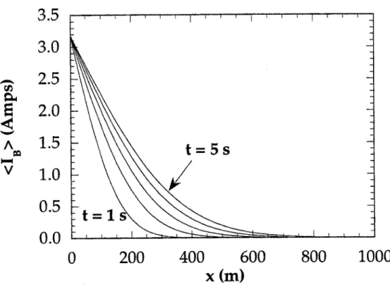
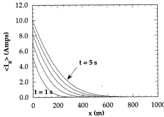
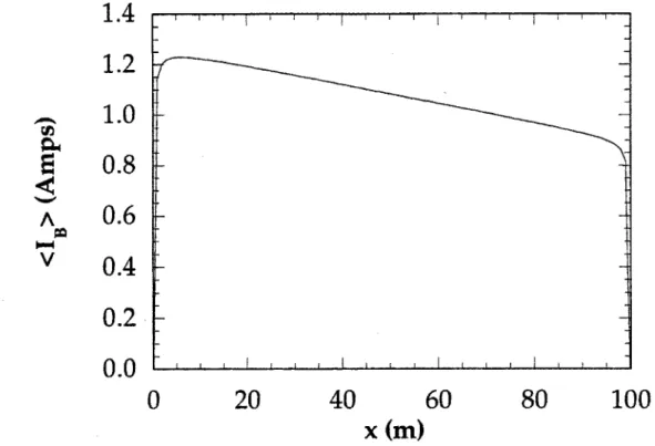
4-1 Example of circulating current in the Infinite Length, Open-Circuit Joints Regime. . . . . 72

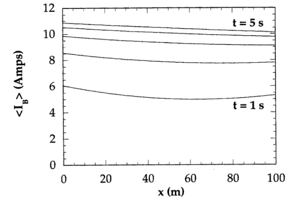
4-2 Example of circulating current in the Infinite Length, Resistive Joints R egim e. . . . . 74

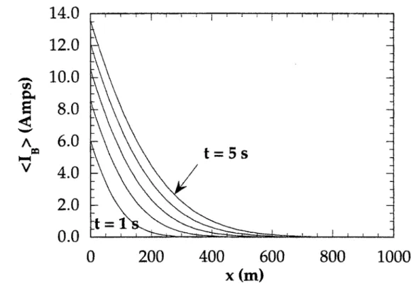
4-3 Example of circulating current in the Infinite Length, Short-Circuit Joints Regime. . . . . 76

4-4 Example of circulating current in the Short Length, Open-Circuit Joints R egim e. . . . . 81

4-5 Example of circulating current in the Short Length, Resistive Joints

Regim e. . . . . 83

4-6 Example of circulating current in the Short Length, Short-Circuit Joints Regim e. . . . . 86

4-7 Example of circulating current vs. time in the Short Length, Short-Circuit Joints Regime. . . . . 87

4-8 Example of circulating current in the Finite Length, Open-Circuit Joints Regim e. . . . . 92

4-9 Example of circulating current in the Finite Length, Short-Circuit Joints Regim e. . . . . 95

4-10 Example of circulating current in the Finite Length, Resistive Joints R egim e. . . . . 98

4-11 The 3 x 3 matrix of operating regimes. . . . . 101

5-1 Non-linear strand resistance, R, per length. . . . . 109

5-2 Cross-section of two-strand model geometry . . . . 111

5-3 The onset of the Resistive Domain occurs when the strand current profile intercepts the critical current profile at t = t. . . . . 126

5-4 Time evolution of Ii(x = £/2,t), I2(x = t/2,t), I,(x = /2,t), and IT/2(t) in the Superconducting Domain. The Resistive Domain begins att=t,... ... ... 127

5-5 Current profiles for strands one and two during the first 5 ms of the Resistive Domain. . . . . 128

5-6 Temperature profiles for strand one during the first 5 ms of the Resis-tive Dom ain. . . . . 129

5-7 Critical current profiles for strand one during the first 5 ms of the Resistive Domain. . . . . 130

5-8 Time evolution of the temperatures, T1, T2, Th at x = f/2. . . . . 130

5-9 Time evolution of the strand one current, 11, and critical current, I, at x = t/2. . . . 131

5-10 Time evolution of the strand two current, 12, and critical current, I,

at x = /2. . . . . 131 5-11 Time evolution of the combined local Joule heating in strands one and

two (i.e. R12I + IZ2I) at x = ./2. . . . . 132

6-1 The strand one current and critical current for the hypothetical cable in the Superconducting Domain. . . . . 148

6-2 The strand currents and the critical current for the hypothetical cable in the Resistive Domain. Unstable case. . . . . 148

6-3 The strand and helium temperatures for the hypothetical cable in the Resistive Domain. Unstable case. . . . . 149 6-4 The strand one current and critical current for the hypothetical cable

in the Superconducting Domain. Stable Case. . . . . 150 6-5 The strand currents and the critical current for the hypothetical cable

in the Resistive Domain. Stable Case. . . . . 151 6-6 The strand and helium temperatures for the hypothetical cable in the

Resistive Domain. Stable Case. . . . . 151 6-7 The strand one current and the critical current for the hypothetical

ca-ble as it cycles between the Superconducting Domain and the Resistive D om ain. . . . . 152 6-8 The strand and helium temperatures for the hypothetical cable as it

cycles between the Superconducting Domain and the Resistive Domain. 153

6-9 Strand temperatures for the hypothetical cable during the first blip for three cases: A, unstable; B, stable; and C, marginally stable. . . . . . 154

6-10 The marginal stability line for the hypothetical cable. . . . . 155 6-11 Analytical results for time 0 < t < t,. The solutions from Chapter 4

can be used to calculate t,, I, and B, = bjt.. . . . . 161 6-12 Examples of overdamped, critically damped, and underdamped

6-13 Examples of recovery, quench, and the marginal stability limit for the case of underdamped behavior. . . . 164 6-14 Comparison of the Marginal Stability Line as calculated using the full

non-linear model, the linear model, and the approximation to the linear model. ... ... ... 165 6-15 Marginal stability plot for hypothetical lab-scale cable using linearized

model equations. View I. . . . . 166 6-16 Marginal stability plot for hypothetical lab-scale cable using linearized

model equations. View II. . . . 168 6-17 Marginal stability plot for hypothetical lab-scale cable using linearized

model equations. View III. . . . 168 6-18 Marginal stability plot for hypothetical lab-scale cable using linearized

model equations. View IV. . . . 169 7-1 Schematic cross-section of the 225 strand US-DPC cable. highlighting

two of the five final stage "sub-cables". . . . 173 7-2 Schematic of one section of the US-DPC cable with terminations. . . 177 7-3 Cross-ssection of the "lap" joint configuration used to join sections of

the US-DPC cable. . . . . 178 7-4 The three regions of the US-DPC cable model: 2 joints and the cable

itself. . . . . 180 7-5 The contour of integration necessary to determine the second interface

condition. . . . . 181 7-6 An example of the induced current per strand in the three regions of

the US-DPC model cable. . . . . 185 7-7 Critical current per strand, I, for the US-DPC vs. magnetic field at

the temperature T = 4.5 K. . . . . 188

7-8 Quench current per strand, 1q, vs. ramp time, t,,p, for the US-DPC

7-9 DC quench current per strand, Iq, vs. quench field, Bmax, for the lab-scale cable test. . . . 193 B-i The random variable x vs.

E

List of Tables

4.1 Definition of Cable Length Classifications. . . . . 65

4.2 Definition of Joint Classifications. . . . . 66

4.3 Cable parameters used in examples for Infinite Cable Length Regime. 70 4.4 Cable parameters used in examples for Short Cable Length Regime. 78 4.5 Cable parameters used in examples for Finite Cable Length Regime. 89 5.1 The Hypothetical Full-Scale Cable Properties. . . . . 125

6.1 The Hypothetical Lab-Scale Cable Properties. . . . . 146

6.2 Restrictions in effect for the linearized stability analysis. . . . . 157

7.1 Selected US-DPC Cable Properties. . . . . 174

Chapter 1

Introduction

Next generation fusion devices such as ITER' are relying on superconducting magnets consisting of Cable-In-Conduit Conductors (CICC) to provide the "magnetic bottle" needed for plasma confinement. In recent experiments however [1, 2, 3], CICC mag-nets have exhibited lower than expected limiting currents when operated in transient magnetic fields. While magnet designers are confident they can build robust mag-nets which will be immune from this so-called "Ramp-Rate Limitation," a thorough unerstanding of the physical mechanisms which cause this phenomenon could lead to better (i.e. less costly) designs.

The main goal of this thesis is to provide a solid foundation for the study of what is now believed to be the principal cause of ramp-rate limitation in CICC magnets, namely, uneven current distribution within the cable [4, 5, 6]. While the effects of current distribution have been studied before (see, for example, [7, 8, 9]), the theoretical analysis in this thesis for the first time begins with a self-consistent physical model which couples the electromagnetic and thermal equations which govern current distribution and stability in superconducting cables.

The thesis takes the philosophical approach of trying to explain the important physical insights in the simplest terms possible. For this reason, the geometrical com-plexity of actual multi-strand cables has been abandoned in favor of a two-strand

analogy which has the dual advantage of being mathematically tractable and physi-cally intuitive. And despite its relative simplicity, the two-strand model contains all of the relevant physics needed to explain the detrimental effects of current distribution in larger cables.

1.1

Overview

The remainder of this chapter provides some general background on superconductors in general, and CICC applications in specific. A description of the relevant material properties and typical design configurations is followed by an introduction to the concept of stability in Section 1.2.1. At the end of the chapter, a brief review of the history of the ramp-rate limitation phenomenon is given.

Subsequent chapters focus on the modeling of current distribution and its effects for CICC. Chapter 2 provides an overview of the theoretical constructs used through-out the thesis and introduces the concept of circulating currents, the root cause of current imbalance within CICC. Despite their importance, circulating currents have previously been largely ignored in the literature; it is believed that this thesis provides the first comprehensive treatment of this topic.

In Chapter 3, the two-strand model which provides the theoretical framework used throughout the thesis is developed. In Chapters 4, 5 and 6, solutions to the two-strand model equations are found for differing operating scenarios. For the first time, important scaling laws are identified which allow the characterization of cables into classes which depend on length, joint design and transverse conductance. Important differences exist between the classes. One important finding is that "full-scale" cables are difficult to simulate with "lab-scale" experiments.

In Chapter 7, heuristic modifications to the two-strand model are made to allow a comparison of the theoretical analysis to experimental results. Despite the inherent limitations of the two-strand model, the theory qualitatively agrees with experiment for the two cases cited. While the theory would need to become more sophisticated in order to achieve a better correlation with the data, the results as presented are

Figure 1-1: An example of a Cable-in-Conduit Conductor (CICC) shown in cross-section. Typically, the strands are twisted into triplets which are further twisted into bundles which are then twisted into sub-cables and so on until the entire cable is formed. Each strand consists of numerous superconducting filaments (not shown in this figure) [10].

sufficient to corroborate the hypothesis that circulating currents account for the ramp-rate limitation experienced in CICC magnets.

The thesis concludes with a summary of the major findings and suggestions for future work in Chapter 8.

1.2

Background

A CICC cable is composed of multiple strands of conductor, each of which is composed

of numerous superconducting filaments embedded in a non-superconducting matrix, typically made of copper. The strands are twisted together and compacted within a structural conduit which provides a passage for a suprcritical helium coolant. A cross-section of a typical CICC is diagrammed in Fig. 1-1. This section reviews the relevant features of cable-in-conduit conductors (CICC's) and introduces the concept

Figure 1-2: The critical surface plot for a commercially available Nb-Ti alloy. At operating points below the surface, the alloy is superconducting; above the surface, it is normal. Source: reprinted with permission from Wilson, Superconducting Magnets, Copyright

@1983

1.2.1

Basic Properties of Superconducting Materials

Superconducting materials exhibit their unique properties when operated within cer-tain limits. Traditionally, these limits are defined as the critical temperature, T,, the critical current density, J,, and the critical magnetic field, B,. These three quantities are interdependent and form a three dimensional "critical surface" in a phase space with coordinates of temperature, magnetic field, and current density. The critical surface defines the boundary between the superconducting state (below the surface) and the normal state (above the surface). The critical surface can be considered a material property of the superconductor although it is also affected by manufacturing techniques. The critical surface for a typical Nb-Ti alloy is shown in Fig. 1-2 as an example.

Any superconducting device must be designed so that the superconductor remains "comfortably" beneath its critical surface in the T, B, J-phase space. Any disturbance in temperature, field, or current density which moves the operating point above the

critical surface will cause the superconductor to go normal. This process is commonly called "Quenching." The stability of the device against quenching is directly related to how close the nominal operating point is to the critical surface.

The properties of a material in the superconducting state are very different from its properties in the normal state. For stability analysis, the most important difference is the sudden change in the electrical resistivity. Surprisingly, most materials which possess a zero-resistivity superconducting state have relatively high resistivities in the normal state. At cryogenic temperatures, the normal state resistivity of practical su-perconductors is 10 - 100 pQ-cm while, for comparison, the resistivity of copper is less than 0.1 uQ-cm [11]. For this reason, and since superconductors are usually operated at very high current densities (often greater than 10' A/m 2 [12]), any local transition to the normal state will be associated with tremendous Joule heating. Such local Joule heating would quickly and irrevocably drive the surrounding superconductor above the critical temperature and into the normal state.

To mitigate this "catastrophic" effect, superconducting wires are formed as a composite material: superconductor filaments embedded in a stabilizer. In the event of a local normal zone in the superconductor, the current can flow around the high resistivity region by traveling through the stabilizer (typically made of copper). The Joule heating associated with a normal zone is thus greatly reduced. In a good design, a coolant (typically suprcritical helium) will be able to absorb the heat generated and cool the strand back down to the operating temperature, where it will again be superconducting. This is known as "Quench Recovery."

A stability analysis of a superconducting system determines the size of disturbance which will cause a "Quench" and whether it will lead to a "Quench Recovery" or a full quench of the entire conductor. Traditional stability analyses usually study the stability of a conductor with respect to disturbances in temperature; the current density and magnetic field are assumed to be uniform and constant. Computer codes such as HESTAB [13] iteratively determine the minimum disturbance energy which would cause the wire to Joule heat to a point where the temperature remains above the critical temperature despite convective cooling provided by the suprcritical helium.

The applicability of such a stability analysis to the problem of ramp rate limitation will be briefly discussed at the end of this chapter in Section 1.2.3.

1.2.2

Cable-in-Conduit Conductors

Cable-in-Conduit Conductors (CICC's) were developed at MIT in the mid-1970's as the initial step in developing large superconducting magnets for fusion reactors and magneto-hydrodynamic (MHD) generators [10]. In the CICC design, multiple strands of superconducting wire are cabled together and enclosed in a conduit which provides structural support as well as a leak-tight passage for helium coolant. The principal advantage of this geometry is that the surface area to volume ratio is much higher than that of a "monolithic" design. The increased surface contact with the helium coolant provides improved stability with respect to perturbations in temperature. This and other advantages of CICC's for large scale applications are discussed in Hoenig [10].

The multiple strands of a CICC introduce new concerns for magnet applications. Unless completely insulated, the strands are in electrical contact with their neighbors and there are paths for currents to flow from strand to strand. If the strands are not twisted, induced loop voltages will be proportional to the field rate of change and to the dimensions of the cable (Faraday's Law). Since cables can be very long, signif-icant induced voltages can occur even for small-diameter cables in slowly changing fields. These voltages will drive eddy currents which travel along the length of one superconducting strand and return down the length of a neighboring strand. The only resistance encountered is at the contact points where the current traverses strands. If this resistance is low, notable eddy currents can exist and the resulting Joule heating will significantly contribute to the AC losses in the cable. This loss must be compen-sated by additional cooling to maintain the conductor below the critical temperature

[12].

AC loss is a particular concern for AC magnets, but is also of interest for DC magnets which must be brought from zero magnetic field to their operating magnetic field in a reasonable amount of time. Fortunately, twisting the strands together effectively reduces the magnetic coupling between strands, putting a handle on AC

loss. Twisted strands in a changing external magnetic field experience an electric field which changes direction every half twist pitch length. The maximum induced voltages will thus be proportional to the twist pitch length rather than the length of the cable [12].

Another way to reduce the coupling between strands is to decrease the conductiv-ity between them. The optimum choice of electrical conductivconductiv-ity between the strands balances the requirement of low AC loss (low conductivity) and adequate stability (high conductivity-to ease current transfer around local normal zones) [12]. For mag-nets that are designed to be ramped or cycled in time, AC loss is a primary concern and highly resistive oxide coatings are often used. Completely insulating the strands from each other is an option, but experience has shown that the performance of such magnets can be "surprisingly low" [14].

Although a simple twisting of all the strands, as diagrammed in Fig. 1-3, reduces eddy currents due to transverse magnetic fields, it does not help to reduce self-field effects. The self-field is the magnetic field of a wire generated by the transport current flowing through it. The self-field effect in multi-strand cables is similar to the "skin-effect" in homogeneous conductors-a diffusion process in which any change in current distribution begins at the surface and diffuses inward at a rate inversely proportional to the conductivity [15]. By analogy, any change in the current distribution in a simply twisted cable will first be felt by strands on the outside before diffusing inward. The superconducting nature of the strands would severely limit the rate at which the currents diffused. The resulting current imbalance would significantly reduce the overall performance of the cable.

A "fully transposed" cable, however, is one which eliminates the self-field effect by ensuring that no net self-field flux exists between the strands [12]. This is equivalent to saying that the self-inductance of every strand is the same and that the mutual-inductances between strands exactly balance. This can be achieved by a cabling pattern in which the strands traverse the cable cross-section in such a way that each spends an equal amount of time at each position in the cable space-i.e., the strands spiral radially inward then outward along the length of the cable.

Figure 1-3: Sketch of a "simply twisted" cable. Strands on the outside remain on the outside over the length of the cable. Strands near the center stay near the center [16].

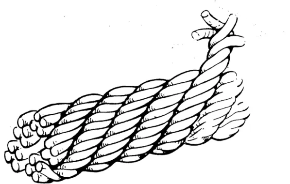
One such cabling pattern which achieves a fully transposed geometry is a derivative of the Litz wires often used for radio frequency work [12]. It begins by twisting a small number of wires into a "rope" with a tight twist pitch. Then several small ropes are twisted together with a somewhat looser twist pitch into a bundle. The process continues, twisting bundles into larger cables with looser twist pitches. An example of a cable made of five ropes of four strands each is shown in Fig. 1-4. The Cable-in-Conduit Conductors discussed later in this thesis are similarly comprised of multiply-twisted strands.

1.2.3

Ramp-Rate Limitation

To demonstrate the ability of CICC magnets to operate at the conditions required for a fusion device, the United States Demonstration Poloidal Coil (US-DPC) was designed and built by MIT and industrial partners. Tested in Japan in late 1990, the magnet performed well in DC tests but exhibited an unexpected ramp-rate limitation when ramped at high rate to high currents and fields. Figure 1-5 shows the measured

Figure 1-4: Sketch of a "fully transposed" cable in the form of a multiply twisted "rope." Source: reprinted with permission from Wilson, Superconducting Magnets, Copyright

@1983

limit for linear current ramping as a plot of maximum attainable current versus the ramp time taken to reach that current. It is evident from the figure that the design current of - 30 kA could only be reached at slow ramp rates (i.e., longer ramp times) despite the fact it was designed to ramp to full current in approximately one second

[1].

The results of the US-DPC experiment were extensively studied using the tra-ditional stability analyses referred to in Section 1.2.1. As mentioned above, these analyses study the stability of a conductor to disturbances in temperature by de-termining if the cooling (heat transfer to helium) is enough to bring the conductor back down to its operating temperature after any foreseeable perturbation in tem-perature. Such perturbations would be caused by energy deposited in the strands from such causes as AC losses, nuclear heating, or frictional heating associated with wire motion. For this reason the measure of stability of a cable is often given as a

35

30

25

20

15

10

5

0

0

2

4

6

8

10

t

I

7

6

5

4

3

2

1

0

2

(s)

Figure 1-5: Quench current vs. ramp time for the US-DPC experiment. The time evolution of the transport current and magnetic field are also shown (inset). The degraded performance at faster ramp times is known as the "Ramp-Rate Limitation." [1]

B

to a non-recovering quench, typically measured in mJ/cc of wire [17].

In studies of the US-DPC coil, however, the stability margin was found to be on the order of 100 mJ/cc for operating scenarios at which premature quench was experienced [18]. This amount of energy is much larger than any foreseen energy deposition in the system, leaving the source of ramp-rate limitation a mystery [1].

What the traditional stability analyses fail to consider, however, is the possibility of non-uniform current distribution within the cable. The remainder of this thesis is devoted to modeling the current distribution to be expected in CICC cables and assessing the effects of this distribution on the stability of the magnet. By the end of the thesis, we reach the conclusion that non-uniform current distribution indeed accounts for the performance limitations encountered in the US-DPC as well as nu-merous follow-up experiments.

Chapter 2

Current Distribution in CICC

Cable-in-Conduit Conductors (CICC) have been used in numerous devices since they were first introduced in the nid-1970's [10]. Accordingly, the literature contains many reports of both experimental and theoretical studies of the performance of CICC's in varying conditions. Until recently, however, nearly all of these studies were predicated on the assumption that the current distribution among the cabled strands was nearly uniform. While this assumption is valid in many cases and leads to numerous useful results, its validity breaks down in the presence of pronounced transient fields.

This preliminary chapter offers a broad overview of the different sources of current distribution in CICC and defines certain concepts which will be used in later chapters. Unfortunately, the few researchers who have focused on non-uniform current distri-bution ([4, 7, 8, 9, 19], for example) have not yet reached a consensus on terminology. The terms chosen for this thesis are for the most part consistent with the literature but are defined below for further clarity.

The overall current distribution is a combination of the directly applied (transport) current and the induced currents. While it is convenient to distinguish between the different sources of current flow within a CICC, it must be remembered that the total current at a certain location is a superposition of the individual components.

2.1

Current Distribution within Composite

Super-conductors

In isolation, a single strand of composite superconductor looks like a complete cable unto itself. The strands are composed of tens to hundreds of superconducting fila-ments imbedded in a metallic matrix (usually copper). Although the filafila-ments are not transposed, they are twisted in a helical manner to minimize the effects of transverse fields. The electrodynamic behavior of single strands in changing magnetic fields has occupied researchers since the fabrication technique was invented and still attracts as much or more attention than the study of CICC's or other cabled conductors. At this point, though, the physics of single strands is fairly well understood and several comprehensive references are available [12, 20, 21].

For the purposes of studying current distribution in cables, however, the individual strands can be treated in a macroscopic sense [22]. In other words, details of current distribution within each strand are not necessary.

2.2

Distribution of Transport Current

The transport current is defined as the net current passing through the cable and is generated by the magnet power supply. The cable is connected to the power supply through a low resitance joint at either end. Joint design is a topic within itself and much research is currently being done to optimize joints for cables in pulsed or ramping fields [23]. One goal of joint design is to insure each strand in the CICC is connected through the same resistance to the power supply leads. Such a joint would produce, in steady-state, a uniform transport current distribution throughout the cable.

For the purposes of this thesis, it is in fact assumed that the effects of unequal strand-to-joint resistances are minimal. Thus, the current distribution due solely to the transport current is considered uniform for each strand. As previously mentioned, though, the overall current distribution is not uniform because of the induced currents

which will be discussed next.

2.3

Induced Currents

Transient magnetic fields cause induced current loops within CICC cables even though the strands are twisted to minimize such effects. In this thesis, the induced current is divided into two components: interstrand coupling currents and circulating currents. The interstrand coupling currents are the more familiar of the two but it is the circulating currents which are of primary interest in this thesis.

2.3.1 Interstrand Coupling Currents

Coupling currents are well-known to anyone who is familiar with composite super-conductors. Just as transverse fields induce coupling currents in a single strand of a composite superconductor, they also induce interstrand coupling currents in a large cable of twisted strands.

The primary effect of these unwanted induced currents has long been known as "A.C. Loss," the Joule heating associated with eddy currents induced by changing transverse magnetic fields. This effect has been extensively studied for composite strands [20, 21] and cables [24] and can largely be understood without regard to how the cable is terminated.

As mentioned in Section 1.2.2, the characteristic length of the interstrand coupling currents is the twist-pitch length of the cable which determines the distance over which the coupling currents reverse direction. The maximum interstrand coupling current density in a strand is generally several orders of magnitude less than the transport current density and thus they do not noticeably contribute to imbalances in the overall current density of the cable. Section 4.2 goes into further detail about how interstrand coupling currents are nonetheless important in determining the boundary conditions which influence the circulating currents, which are discussed next.

2.3.2

Circulating Currents

Like interstrand coupling currents, circulating currents are induced by changes in the magnetic field. Circulating currents, however, have a characteristic length much longer than the longest twist-pitch length and can appreciably alter the overalll dis-tribution of current density in the cable. In fusion magnets, circulating currents are mainly a result of the low resistance joints through which the cables are connected to the power supply. These low resistance paths can locally "undo" much of the benefit of subdividing the superconductor into twisted strands. In abstract terms, circulating currents can be thought of as the component of the total induced current distribution which passes through one or both joints.

In mathematical terms, circulating currents are driven by the end "boundary conditions." Depending on the properties of the cable, they can be isolated near the ends of the cable or they can join to form a "loop" current which changes the current distribution over the whole length of the cable. The concept of circulating currents is developed much more rigorously in Chapter 4.

2.4

Current Redistribution during Quench

The individual aspects of current distribution discussed so far-transport current, interstrand coupling current, circulating current-all presume the cable is operating in the superconducting state, as defined in Section 1.2.1. When all or a portion of the cable enters the normal state, the current distribution can change quickly and dra-matically. For normal regions which occupy only a portion of the cable cross-section, current transfers from over-saturated strands to strands which are still supercon-ducting. If the entire cross-section quenches over a long enough length, the higher resistance of each strand damps out the induced current effects described above and the current distribution becomes almost uniform.

In general, the redistribution of current due to quenching of the cable is non-linear in nature and requires a coupled solution of the time-dependent thermodynamic and electromagnetic behavior of the cable. This aspect of the stability analysis is dealt

with in Chapter 5.

2.5

Summary

The overall distribution of current in a CICC is influenced by three distinct compo-nents: the transport current, the interstrand coupling current, and the circulating current. Of these three, the last is in many ways the least understood-it is certainly the least studied.

Circulating currents are induced by changes in the magnetic field but behave much differently than the eddy currents traditionally considered in AC loss analyses. In some situations, the uneven distribution of current caused by circulating currents can be appreciable and should be of concern to magnet designers. The remainder of this thesis is devoted to explaining these circulating currents and their effect on the

Chapter 3

The Two-Strand Model

This chapter focuses on the development of a two-strand model of current distribution in cables exposed to ramping magnetic fields. At first appearance, the model seems rather simple but the results derived from the two-strand example exhibit surprisingly complicated behavior. In later chapters, the model presented here will be shown to self-consistently explain much of the "anomalous" behavior witnessed in cables exposed to ramping magnetic fields.

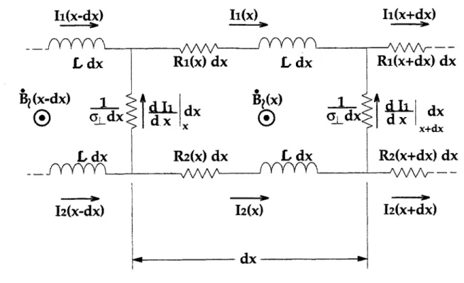
This chapter begins with a discussion of the relative merits of the two-strand model over the more ambitious approach of solving the problem for an actual cable geometry. Next, a physical description of the two-strand cable is given and key attributes of the cable are identified. The cable is then analyzed on a differential scale from which the electromagnetic diffusion equations at the crux of the model are developed.

Although the temperature-dependent resistive elements in the model are included for completeness sake, the coupling of the circuit equations with the heat equations will not be presented until Chapter 5. The auxiliary equations needed to describe the strand resistance and the behavior of the critical current density are presented in that chapter, as well.

3.1

Simple vs. More Complicated Cables

The current distribution in a cable-in-conduit superconductor is difficult to analyze due to the complicated twisting geometry of the strands. For the purposes of analyzing stability and studying ramp-rate limitation, however, it is instructive to simplify the cable geometry as much as possible while still retaining the important physics of the problem. For this reason, it was decided to develop the foundation of the analysis using a two-strand model. This decision seems especially justified since the two-strand results developed in this thesis are already significantly more elaborate than those of previous studies [17, 25, 13]. The complexities of a fully-transposed multi-strand cable are best left for the next "iteration," should more detail be deemed necessary. The advantages of first studying a two-strand model are strong ones. Most im-portant, the mathematics of the two-strand model are relatively straight forward and do not cloud the underlying physics. In studying a full-sized CICC, it is necessary to use a continuum model and very sophisticated numerical techniques. Actually, in many circumstances, it is not even clear if such techniques exist. After studying the problem extensively, this author concluded that even if a solution were to be found, it would not be the best way to convey the important results which can be demonstrated with the simpler two-strand model.

The two-strand model offers a physically intuitive way to understand the sources of current distribution in superconducting cables. Although the model does not account for the full geometrical complexity of a full-scale cable, the results nonetheless shed light on many previously unappreciated aspects of current distribution and stability. Since the model can be studied analytically, it is possible to develop important figures-of-merit and scaling laws which can be used to classify the behavior of differing cable designs.

It is important to point out that the two-strand model is self-consistent; it does not rely on unknown or outside heat sources to initiate the quench and determine the stability of the cable. The only source of instability is the current re-distribution which is caused by a ramping magnetic field. If one were to actually construct a two-strand

cable, the analysis presented in this thesis would accurately predict its behavior. The extension of the analysis to multi-strand cables is the subject of Chapter 7.

3.2

Two Strand Model Geometry and Properties

Before discussing the details of the two-strand model, it is necessary to give a brief physical description of the model in order to put the problem into context. The cables being considered in this thesis are typically wound into solenoidal coils. Rather than explicitly retaining the winding shape, however, the coil is considered to be straight and parallel to the x-axis. The effects of the winding are included through the spatial dependence of the magnetic field, (see Section 3.3.4).

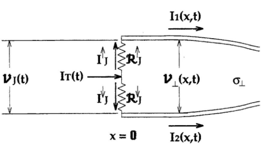
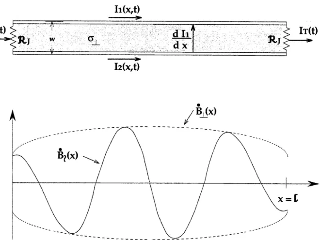
The geometry of the two-strand model is diagrammed in Fig. 3-1. The individual elements of the model will be discussed thoroughly in the next section but the diagram and following description offer an overview. The two strands are twisted together in a double helix with characteristic twist-pitch length, tp, and distance between centers, w. In the figure, the strands are drawn as one-dimensional "filaments" even though they actually have a strand diameter, d. The total length of the cable is and the two strands are connected to the power supply at either end through low resistance joints with transverse resistance, Ri. The cable experiences a transverse magnetic field density, Bi(x, t), that is in general a function of space and time. Along the length of the cable, the transverse electrical conductance-per-unit-length is ai. The value of

oI represents the conductivity of the medium which separates the two strands. This medium could be vacuum, for instance, or the other strands of a full cable, which we can treat as a medium with known properties.

To give an idea of the physical scale of the problem, the cables considered in this thesis will vary in length from t= 1 to 100 m; the typical twist-pitch length will be of the order

4p

x=E

A

x

=

x=E

Figure 3-1: The two-strand model geometry. The two strands form a double-helix with a constant width w. _{Also shown is an example of the magnetic field profile,}

B(x,t).

B(x,t)

3.3

Notation and Parameters

At this point, we need to introduce the parameters and notation which will be used throughout the thesis. In later chapters, new notation will be defined as needed, but the definitions given here will hold true "globally."

3.3.1

Currents

The most important quantity in any discussion of current distribution is of course: current. As was discussed in Chapter 2, the total current in the cable can be thought to consist of several components. For the ease of mathematics and the ease of pre-sentation, it will be useful to define separate notation for each component.

In general, the symbol I will be used to represent current in units of Amps. Since it is necessary to differentiate between the currents in each strand, the subscripts 1 and 2 will represent the first and second strand, respectively. Strand one will be defined to be the strand with the greater current-i.e. 11 > 12.1 Because the strands are not insulated over their length, I1 and I2 are functions of axial location, x, and time, t.

Critical Current

Besides the strand currents, the study of current distribution and stability also in-volves another "current"- the critical current, I,. The critical current is not actually a physical current but rather a definition of a limiting value for the current in the strands: when 11

<

together the current and heat equations which comprise the two-strand model. The role of the critical current is discussed extensively in Chapter 5.

A simple model of the critical current which is appropriate for a single wire of type II superconductor was proposed by Kim [26]:

Ic(T, B) = /B (3.1)

where is a property of the strand (units AT) appropriate for a fixed temperature, Tb. The effects of temperature can usually be well approximated with a linear dependence

(truncated at zero) [12], giving:

& (1 - T~~T ) T < Tc(B)

I,(B,T) = T,-Tb (3.2)

0 T > Te(B)

where the critical temperature, T, is a function of the magnetic field:

J

Tc(B) = 'CO (3.3)

Tb B > Bo

and Tco and Bco are characteristic properties of the superconductor which usually need to be determined experimentally.

This modified Kim's model, Equation (3.2), will be used in Chapters 5 and 6 to characterize typical Nb3Sn conductors which have been used in numerous experiments

[4, 5]. The appropriate values for the superconductor properties in this instance are:

= 1250 AT Teo = 18 K B o = 19 T0

The results developed in future chapters can be easily generalized to other super-conductors which obey the modified Kim's model as well as supersuper-conductors with altogether different critical current characteristics.

Transport Current

When both strands are superconducting, it is useful to make the distinction between the induced current component and the transport current component of each of the strand currents. The transport current, Ir(t), is defined as the total net current flowing through the cable: IT = I, + 12. _{It is a known quantity which does not}

vary over the length of the cable (due to current conservation) but can be time dependent. In a coil generating its own magnetic field, IT(t) is directly proportional to the peak magnetic field, B(t). For cables inserted into background field coils, however, IT(t) is independent of the magnetic field and can be an arbitrary function of time. For instance, we will later study cases for which the transport current is constant, IT(t) = IT, while the background field is ramped.

For the purposes of this thesis, the total transport current in the cable will be evenly divided between the two strands.2 _{For the sake of convenience, then, the}

notation IT/2 is used to designate one-half the transport current, i.e. IT/2(t) =

}Ir(t).

Thus, in the absence of magnetic fields (and in the case 11 < I), the current in each strand would be: I,(x, t) = 1₂(x, t) = IT/2(t).

Induced Currents

With the introduction of a ramping magnetic field, however, induced currents must now be considered as well as transport currents. The induced currents in strands one and two are labeled IBI(x, t) and IB2(X, t), respectively. Notice that unlike the transport current components, the induced currents are functions of x as well as t. The total current in each strand is the combination of the transport current and the induced current:

Ii(x,t) = IT/2(t)+IB1(xt)

I2(x,t) = IT/2(t)+IB2(xt) 2

The model could easily accommodate the more general case with the transport current not

divided evenly between the two strands, but the maldistribution of transport current is not the focus of this thesis.

where, again, we are now only discussing the I < 1, scenario. Adding these two equations and noting that IT/2 = 1Jr(t) and IT I1 + 12 (by definition) yields the

expected but important result:

IB1(X, t) - IB2(x, t) = 0 (3.4)

This conservation law implies that any x-dependence of the induced current IBimust be matched by the opposite dependence in IB2. In other words, the current "exiting" strand one at location x flows across the cable and "enters" strand two at the same x location. Mathematically, this is stated as:

aIB1 (X, t) IB2(X, t)

9x 8x

Transverse Current-per-Unit-Length

The quantity -IBI(x,t) has the units [A-m-1] and is the transverse current-per-unit-length flowing between the strands at location x. Since the medium between the strands is resistive (see 3.3.3), this transverse current produces Joule heating. The study of such interstrand coupling losses has been treated by several authors interested in AC losses [24] but does not play an important role in the stability model being developed here.

In cases where 1, is no longer less than Ic, the distinction between transport current and induced currents is no longer useful and the transverse current-per-unit-length then includes the quench redistribution current (see Section 2.4) as well as the induced currents. Thus, to develop the general case, the more general notation

S11(x, t) will be used throughout the remainder of this chapter.

Shorthand Notation for Currents

Since 11 and 12 are easily related, 1 + 12 = IT, we often focus only on 1 and drop the subscript: I = I,. The transverse current-per-unit-length is also shortened to

and 8IB to replace BI and 131.

3.3.2

Inductances

For the purposes of calculating inductances, the cables are considered to be straight, parallel cylinders. The necessary condition for this approximation to be valid is: w/4,

<

The mutual inductance-per-unit-length of two parallel cylinders is given by: [27]

M=0.2 In -+ 1+- - 1+-+-

w 22

where £ is the length and M is in units of [pH -m-11. In the limit under consideration, w/£

<

2f

M = 0.2 In -_- 1

The self-inductance-per-unit-length for a straight cylinder is: [27]

',= 0.2 In 2 _

I r 4

where r is the radius of the cylinder and L, is in units of [pH -m-1]. The quantity of interest for the model turns out to be the "effective" inductance, C =

4,

M.

L = 0.2( + In)

\4 r)

This is the relation which will be used throughout the rest of the thesis.

3.3.3 Resistances

There are three "flavors" of resistance in the model: transverse joint resistance, trans-verse cable resistance, and strand resistance. Each plays a very distinct role in the

behavior of a cable experiencing a ramping magnetic field.

Strand Resistance

The strand resistances, R1 and R2, axe actually resistances-per-unit-length (9/m):

where 7 is the resistivity and A, is the cross-sectional area of the wire. Since the

wires are composites of superconducting filaments within a conductive matrix, the value of 77 is a volume-weighted average of two resistive paths in parallel:

77=( , (I - A))~

7 7 1

where A is the volume fraction of superconductor in the wire, qm is the resistivity of the matrix material, and 77, is the resistivity of the superconductor.

The value of ?1,c changes dramatically depending on whether the strand current is above or below the critical current:

77sc < , ; 0 < I < I

7c = 7f;0 < Ic < I

e> 0 = c < I

where 77ff is the "flux flow resistivity" which will be discussed in Section 5.2.1. Thus, in general, 77 is a non-linear function: when I is less than I, the strand is supercon-ducting and 77 = 77,/A . When I is greater than I, q begins to increase dramatically,

reaching the value q = 7m/(l - A) in the limit I

>

In the first case, I < I, the value of the resistivity, 77., is known as the "dynamic resistivity" -the resistivity of a superconducting material experiencing a time-varying magnetic field [20, 21]. For typical cases considered here, q,c - 1 0-15- 1 0-1 2m[24]. This translates into: I,, ~ 10-9-10-8 S/mfor typical strand dimensions.