HAL Id: hal-02406554
https://hal.archives-ouvertes.fr/hal-02406554
Submitted on 12 Dec 2019
HAL is a multi-disciplinary open access
archive for the deposit and dissemination of
sci-entific research documents, whether they are
pub-lished or not. The documents may come from
teaching and research institutions in France or
abroad, or from public or private research centers.
L’archive ouverte pluridisciplinaire HAL, est
destinée au dépôt et à la diffusion de documents
scientifiques de niveau recherche, publiés ou non,
émanant des établissements d’enseignement et de
recherche français ou étrangers, des laboratoires
publics ou privés.
To cite this version:
Elia Moscoso Thompson, Silvia Biasotti, Julie Digne, Raphaëlle Chaine. mpLBP: A point-based
representation for surface pattern description. Computers and Graphics, Elsevier, 2020, 86, pp.81-92.
�10.1016/j.cag.2019.12.001�. �hal-02406554�
Contents lists available at ScienceDirect
Computers & Graphics
journal homepage: www.elsevier.com/locate/cag
mpLBP: A point-based representation for surface pattern description
EliaMoscoso Thompsona,∗, SilviaBiasottia, JulieDigneb, Rapha¨elleChaineb
aIstituto di Matematica Applicata e Tecnologie Informatiche ‘E. Magenes’ - CNR bLIRIS, Universit´e Claude Bernard Lyon 1, CNRS, France
A R T I C L E I N F O
Article history:
Received December 6, 2019
Keywords: Computers and Graphics, Shape analysis, Pattern retrieval
A B S T R A C T
The Local Binary Pattern (LBP) is a very popular pattern descriptor for images that is widely used to classify repeated pixel arrangements in a query image. Several exten-sions of the LBP to surfaces exist, for both geometric and colorimetric patterns. These methods mainly differ on the way they code the neighborhood of a point, balancing the quality of the neighborhood approximation with the computational complexity. For instance, using mesh topological neighborhoods as a surrogate for the LBP pixel neigh-borhood simplifies the computation, but this approach is sensitive to irregular vertex distributions and/or might require an accurate surface re-sampling. On the contrary, building an adaptive neighborhood representation based on geodesic disks is accurate and insensitive to surface bendings but it considerably increases the computational com-plexity. Our idea is to adopt the kd-tree structure to directly store a surface described by a set of points and to build the LBP directly on the point cloud, without consider-ing any support mesh. Followconsider-ing the LBP paradigm, we define a local descriptor at each point that is further used to define a global statistical Mean Point LBP (mpLBP) descriptor. When used to compare shapes, this descriptor reaches state of the art per-formances, while keeping a low computational cost. Experiments on benchmarks and datasets from real world objects are provided altogether with the analysis of the algo-rithm parameters, property and descriptor robustness.
c
2019 Elsevier B.V. All rights reserved.
1. Introduction
1
In the plethora of distinctive elements of a 3D model, relief
2
and color patterns are crucial aspects for many applications that
3
require a local object characterization. Examples of these
appli-4
cations are the recognition of natural structures, like trees [1],
5
the analysis of artworks styles [2], the classification of fabric
6
patterns [3] or the categorization of objects [4].
7
Patterns, as meant in this work, are decorative elements that
8
are defined by small corrugations of the surface or simple color
9
∗Corresponding author: Tel.:+39-010-6475-697; fax: +39-010-6475-660;
e-mail: [email protected] (Silvia Biasotti), [email protected] (Julie Digne),
[email protected] (Rapha¨elle Chaine), [email protected] (Elia Moscoso Thompson)
arrangements repeated on the surface. We distinguish two types 10
of patterns: geometric patterns that represent small variations 11
on the surface geometry, e.g., repeated, small incisions, chis- 12
elings, bumps, etc.; and colorimetric ones, e.g., elements with 13
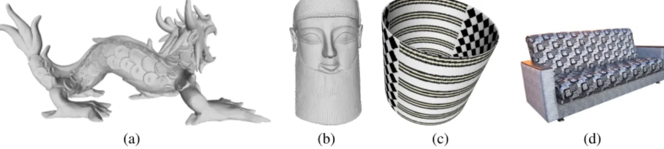
small painted decorations on the surface. Figure 1 shows exam- 14
ples of artworks and design objects characterized by geometric 15
and/or colorimetric patterns. Note that a single element or an el- 16
ement repeated only twice (like the nose or the eyes of a statue) 17
do not represent a pattern. Patterns are among the main fac- 18
tors when characterizing the type, material and style of natural 19
surfaces and many kinds of object decorations, such as archae- 20
ological findings [4]. 21
The analysis of patterns on surfaces is challenging for many 22
reasons, mainly because of the structure of the 3D representa- 23
(a) (b) (c) (d)
Fig. 1. Examples of two surfaces with geometric patterns (a-b) and two surfaces with colorimetric ones (c-d).
cost of the analysis low enough, to be usable in real world cases.
1
The problem of pattern recognition on surfaces is still open [5].
2
In this paper, we tackle the simpler and related problem of
Pat-3
tern Retrieval: we consider models fully covered by a single
4
pattern and our goal is to identify this pattern. Taking
inspira-5
tion from the LBP [6, 7], which was introduced to characterize
6
the binary distribution of the intensities on a ring around one
7
pixel of an image, it is possible to extend it to tackle the
prob-8
lem of surface pattern retrieval.
9
To the best of our knowledge, this has been done in recent
10
years by different authors, culminating in three different
opera-11
tors: the meshLBP [8, 9], the edgeLBP [10, 11] and the Mean
12
Point Local Binary Patterns (mpLBP for short) [12]. All these
13
methods show that it is possible to tackle the pattern retrieval
14
and classification problem using the LBP, with different degrees
15
of success. Even considering other approaches (e.g., the SIFT+
16
Fisher Vector on circular patches adopted in [13]), these
meth-17
ods perform well, marking what is currently the state of the art
18
in this research field. The mpLBP, in particular, yields
excel-19
lent performance scores while keeping low the computational
20
cost. The mpLBP operator defines a LBP-based descriptor able
21
to deal with surfaces represented by sets of points. If the
sur-22
face is given as a tessellation, this set of points can be the set of
23
vertices, possibly supplemented by additional points sampled
24
on the faces if the number of vertices is low (see Section 3).
25
These points are organized in a kd-tree structure, which makes
26
the navigation in the model representation easier and quicker
27
[14].
28
This paper extends [12], providing more discussions on the
29
robustness of the mpLBP descriptor, also considering di
ffer-30
ent surface bendings and presenting the mpLBP performance
31
on models obtained from scans of archaeological fragments.
32
Moreover, we analyze the efficiency of the descriptor and its
33
characteristics when different neighborhood shapes and
sam-34
pling rules are chosen.
35
The remainder of this paper is organized as follows.
Sec-36
tion 2 gives an overview of previous research for the retrieval
37
and classification of patterns over surfaces. Section 3
intro-38
duces the punctual operator at the basis of the description, the
39
mpLBP descriptor and presents four possible variants for the
40
ring sampling. Section 4 presents the mpLBP experimental
set-41
tings, introducing both the datasets and performance measures
42
and the shape properties adopted for the mpLBP computation.
43
Section 5 presents the results of all the tests performed on the
44
mpLBP. In particular, Section 5.1 shows the retrieval and
classi-45
fication performance of the method on two benchmarks [3, 15]
46
and over a set of scans of archaeological fragments. Section 5.2 47
focuses on the method robustness with respect to noise and 48
different surface bendings, while Section 5.3 analyzes on the 49
mpLBP performances with different punctual descriptor sam- 50
pling schemes. Discussions, concluding remarks and feature 51
works are provided in Section 6. 52
2. State of the Art 53
The retrieval and classification of reliefs and textures on sur- 54
faces can be seen as an extension to surfaces of the texture 55
image retrieval problem. A large variety of methods for tex- 56
ture image analysis has been proposed in the literature. The 57
main challenge for the detection of specific texture patterns is 58
the recognition of the texture properties robustly to the possi- 59
ble variations [16]. A typical strategy to detect patterns on im- 60
ages is to consider local patches that describe the behavior of 61
the texture around pixels. Examples of statistical descriptions 62
are the Local Binary Patterns (LBP) [6, 7], the Scale Invariant 63
Feature Transform (SIFT) [17] and the Histogram of Oriented 64
Gradients (HOG) [18]. LBP-based methods are very popular 65
and a large number of LBP variants has been proposed [19]. 66
An extended taxonomy of 32 LBP variations and their perfor- 67
mance evaluation for texture classification has been proposed 68
in [20] where the LBP variations and 8 convolutional network 69
based features are evaluated over 13 datasets of 2D images. 70
Among the LBP variations considered, the overall best perfor- 71
mances are obtained by the so-called Median Robust Extended 72
LBP (MRELBP) that evaluates the descriptor over representa- 73
tive regions instead of single pixels. In terms of absolute per- 74
formances, the method based on CNN and Fisher Vectors [21] 75
obtains the best results but has a considerably higher compu- 76
tational complexity. In parallel, the aggregation of significant 77
feature points obtained by pooling the point descriptors, e.g. 78
SIFT+Fisher Vectors, was evaluated and obtained significant 79
texture classification performances [16]. Similarly to LBP, the 80
combination of a SIFT-based feature description with Convolu- 81
tional Neural Networks outperforms the feature-based descrip- 82
tions on classic benchmarks approximately by 10% at the cost 83
of a higher computational complexity, [21]. 84
For the characterization of patterns over surfaces, two strate- 85
gies have been adopted so far: (i) a reduction of the problem 86
to an image pattern one, for instance with the projection of the 87
data onto an well chosen plane (image) and the application of an 88
image pattern recognition algorithm to the projected data; (ii) 89
fact which is not straightforward because it involves handling
1
of three-dimensional data.
2
As an example of reduction strategy, the method in [1] for
3
tree species classification represents the geometric variations of
4
the tree trunk models with a 3D deviation map over a best
fit-5
ting cylinder obtained with the Principal Component Analysis
6
(PCA) technique. Then, the cylinder is flattened on a plane
7
and the geometric textures are compared using variations of the
8
complex wavelet transform. Similarly, [2] adopts a height map
9
to project the reliefs and engraves of rock artifacts into an image
10
and classify them. The LBPI and CMC approaches proposed
11
in the SHREC’17 contest [3] adopt, respectively, an image
pat-12
tern method over a depth-buffer projection of the surface (LBPI)
13
and the comparison of the principal curvatures in the mesh
ver-14
tices using morphological image analysis techniques (CMC).
15
Recently, [13] has proposed to use an opportune
parametriza-16
tion around a patch centroid to project the mean curvature
val-17
ues into an image and then, to adopt the SIFT+ Fisher Vector
18
[16] strategy to compare the parametric images.
19
The Mesh Local Binary Pattern (meshLBP) approach [22, 8,
20
9, 23] proposed the first extension of the LBP description [6]
21
to triangle meshes. The main idea behind the meshLBP is that
22
triangles play the role of pixels; there, the 8-neighborhood
con-23
nectivity of images is ideally substituted by a 6-neighborhood
24
connectivity of the vertices. The role of the gray-scale color is
25
replaced by a function that is meant to capture the main pattern
26
characteristics (usually Gaussian or mean curvatures, shape
in-27
dex [24] or mesh color if such information is provided). The
28
edgeLBP [10, 25, 11, 3, 15, 4] performs an LBP evaluation that
29
is based on the rings built over the mesh edges. Adopting a
30
surface-aware characterization the edgeLBP is able to
outper-31
form the meshLBP in terms of quality of the query results but
32
it pays a higher computational cost. To overcome the
compu-33
tational limitation of the edgeLBP, the mpLBP has been
intro-34
duced in [12]. In this case, to speed the extraction of the
de-35
scriptor, the mpLBP takes advantage of the kd-tree structure
36
and therefore it deals directly with point clouds.
37
For point clouds, local surface patches can also be
con-38
structed by regression using the neighborhood around one point
39
[26, 27, 28, 29] and those patches can be compared in the
pa-40
rameter space. In most recent approaches, the surface was
lo-41
cally characterized as a digitized height field over the regression
42
surface which may be a plane [30] or a quadric (see [31] for an
43
application to super-resolution).
44
3. mpLBP descriptor
45
This section introduces a statistical descriptor that is global to
46
the shape, that aggregates values of local descriptors computed
47
at a set of positions on the surface. The input surface model can
48
be a point cloud or a triangulation (in the last case, the vertices
49
are input points for the descriptor).
50
The mpLBP procedure can be described by two main steps:
51
the creation of the punctual descriptor (Section 3.1) and LBP
52
evaluations that are further combined to create the mpLBP
de-53
scriptor (Section 3.2). In Section 3.3 we discuss the definition
54
and tuning of the parameters of the method.
55
3.1. Punctual descriptor 56
Let S be a point set embedded in the 3D Euclidean space 57
and a surface property defined on S , h : S → R, a function 58
defined on S whose values depends on the pattern we want to 59
describe (e.g.: curvature-based values in case of geometric pat- 60
terns, a color-based property in case of depicted decorations, 61
etc.). Let us consider the point ˜p ∈ S and the set S [ ˜p] of the 62
points pi ∈ S at a distance from ˜p at most equal to R, i.e., 63
S[ ˜p]= {pi∈ S |d( ˜p, pi) ≤ R}. We will discuss the choice of the 64
radius R in Section 3.3. Gathering the sets S [ ˜p] means visiting 65
the points of S several times. Since 3D models with patterns 66
must be at high resolution (thus described by a high number of 67
points), the way the distance relations between points are com- 68
puted must be efficient. In our implementation, these relations 69
are computed using a kd-tree. This structure is computed once 70
per model (with a computational cost of n log(n)). 71
Points in S [ ˜p] are projected on a plane π, obtained using lin- 72
ear regression on S [ ˜p]. When the density is high enough and if 73
the radius is chosen carefully, that plane may be interpreted as 74
an approximation of the tangent plane. The projected points are 75
sorted in nradconcentric rings based on their distances from ˜p. 76
The number of rings is given by the parameter nrad, that we
call radial resolution. Each ring is defined, for j= 1 · · · nrad, as
follows: S[ ˜p]j= n pi∈ S [ ˜p]|d( ˜p, pi) ∈ [Rj−1, Rj]o , Rj= j R nrad
Each S [ ˜p]jis divided in Pjsectors, delimited y some
regu-larly spaced angle values θk. Note that Pjmay vary along the
rings, in order to obtain sectors with similar areas. We call Pj
the spatial resolution. More formally, we define the sector k of the ring j (sector ( j, k) for short) of the point ˜p as:
S[ ˜p]kj=npi∈ S |d( ˜p, pi) ∈ (Rj−1, Rj], θi∈ (θk−1, θk]o ,
where θk = k2πP
j, k = 1 · Pj. Finally, we assign to each sector 77
( j, k) a value sec( ˜p)k
j as the representative of the function h in 78
that sector. Figure 2 represents the pipeline to build the punctual 79
descriptor. Note that the punctual descriptor can be seen as a 80
feature vector by simply stacking the values of the descriptor 81
on each ring. 82
As it usually happens in the LBP implementations, we ex- 83
cluded the computation of the punctual descriptor at points that 84
are close to the boundary of the model (if any). If the bound- 85
ary of the model is known, it is enough to consider only the 86
points that are at least at distance R from the boundary. In addi- 87
tion, if a point punctual descriptor has more than1 4
P
jPjempty 88
sectors, we considered it invalid and discard that point. When 89
the intersection of the sphere of radius R with the point cloud 90
generates multiple surface components like those in Figure 3 91
(Right), we consider such a configuration non acceptable and 92
refine the point neighborhood by selecting a smaller value for 93
R. Indeed, for a given model M we assume that the projection 94
onto π is injective and that the surface locally captured by the 95
sphere is locally homeomorphic to a topological disk. More- 96
over, we assume the existence of a radius ˜Rmax, which is the 97
maximum value for the parameter R such that all the points on 98
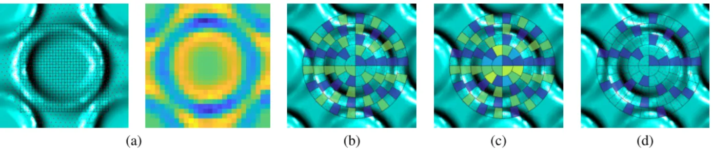
(a) (b) (c) (d) (e) (f)
Fig. 2. A mpLBP descriptor at point ˜p (marked with a light-blue star in (a)). (b): neighborhood S [ ˜p] of ˜p is shown with a dark sphere. (c): point density in S [ ˜p]. (d): regression plane π , (e): clustering into sectors. (f): resulting punctual descriptor, represented as a ’circular’ feature vector.
Fig. 3. Left: illustration of the Gaussian filter adopted to weight the points (in white) in a given sector (in purple). The colors of the Gaussian range from blue (0) to yellow (1). Right: example of a neighborhood that could occur if the radius R is larger than ˜Rmax: points are samples on two
discon-nected parts.
Fig. 4. LBP evaluation for an image. Top-left: in red, the pixel p is high-lighted with a dot together with the circle of radius R centered at p. The values of h around p are reported in the bottom-left image.
3.2. Local Binary Pattern evaluation
1
The punctual descriptor introduced in Section 3.1 is the point
2
neighborhood representation to which we apply the LBP
encod-3
ing technique.
4
The LBP paradigm is very popular for images and many
ver-5
sions are available [19]. We extend the LBP description to
sur-6
faces following closely the image approach [7] which we briefly
7
summarize. For each pixel p, the set of pixels ˜pjwithin distance
8
Rfrom p is called a ring of pixels. Visiting each ring from the
9
top-left pixel in counterclockwise order, a binary array with as
10
many elements as the pixels in the ring is created, adding 0 if
11
h( ˜pj) ≤ h(p) and 1 otherwise. Then the LBP value of p is the
12
sum of the numbers in the binary array (it varies from 0 to the
13
number of pixels in the ring). Note that, in this context, it does
14
not matter the order of the comparisons p and all the ˜pj. The
15
histogram H of the LBP values for all the image pixels is the
16
LBP descriptor of the image. Figure 4 shows this process for a
17
single pixel (Left) and a possible final descriptor (Right).
Mul-18
tiple rings can be considered, increasing the size and descriptive
19
capability of the descriptor.
20
In our case we consider ˜p defined as in Section 3.1. If the radius R is small enough with respect to the curvature and the
thickness of the object, we can suppose that the rings of the punctual descriptor are locally close to concentric rings using geodesic distance to ˜p. Thus, each sector can be seen as the evaluation of h at a sample of the surface. For all the points ˜p in S , we define LBP( ˜p) the feature vector of nrad elements as
follows: LBP( ˜p)j= X k (str[ ˜p]j)k, (str[ ˜p]j)k= ( 0 i f sec( ˜p)k j< h( ˜p) 1 otherwise
Then, the mpLBP descriptor of S (mpLBP(S )) is the his- 21
togram of the LBP values of the points of S . As a final step, 22
the mpLBP is normalized, i.e., all the entries of mpLBP(S ) are 23
divided by the number of points considered in the histogram, 24
enhancing the stability of the descriptor. 25
The mpLBP(S ) is aP
j(Pj+ 1) sized feature vector. Intu- 26
itively, we can visualize it as a horizontal concatenation of the 27
rings of the multiple feature vectors in Figure 2(f). In particular, 28
the j − th ring generates a feature vector of Pj+1 entries, where 29
mpLBP(S )( j,m)is equal to the number of points ˜p in S such that 30
LBP( ˜p)j= m (with j = 1, ..., nradand m= 0, ..., Pj). 31
It is worth mentioning that if the neighborhood of a point is 32
rotated significantly around the normal of the point, its punctual 33
descriptor changes. On the contrary, if the rotation is small, the 34
punctual descriptor is stable; indeed, the Gaussian filter adopted 35
to weight the points is stable under rotations smaller than a frac- 36
tion of the angular sector. In other words, if the grid of sectors 37
(Figure 2(e)) is slightly rotated, the punctual descriptor does not 38
vary significantly. Moreover, we recall that the LBP value per 39
ring (as intended in this paper) is rotation invariant (because it 40
is a sum of 0 and 1 values on the whole ring), we can conclude 41
that the pattern descriptor of the mpLBP is robust to rotations 42
of the surface. This fact has been verified by applying a ran- 43
dom rotation to each point neighborhood: the results indicate 44
almost a perfect stability in this sense. More detail on this fact 45
are provided in Section 5.1. 46
3.3. Parameter settings 47
The three parameters of the mpLBP are the radius R (used 48
to set the neighborhood size around each point of S ), the radial 49
resolution nradand the spatial resolution Pj. This is similar to 50
the parameter set of the edgeLBP as described in [10], the main 51
difference being that for the edgeLBP the parameter P is fixed 52
across all the rings. In the following, we present some hints on 53
how these parameters should be tuned. The intuition suggests 54
that the mpLBP ability of detecting a pattern depends on the 55
must be related to the pattern size. Moreover, the denser the
1
ring sampling, the more complete information is stored, at the
2
cost of a larger storage size.
3
• R: neighborhood radius shown as a dark bubble in
Fig-4
ure 2(b). R should be set so that neighborhoods contain
5
at least one part of the pattern that we want to describe
6
(e.g.: if the pattern is defined by chiseled circles, the
bub-7
ble should contain at least one circle entirely).
8
• nrad: it defines the radial resolution and should be fixed
9
together with Pj(see below).
10
• Pj: it represents the spatial resolution and varies over the
11
different rings.
12
Choice of the rings and sampling scheme. The original mpLBP
13
description proposed in [12] adopts as the point description a
14
set of circular rings such that the spatial resolutions Pj
guar-15
antee that all the sectors have the same area. For this reason,
16
we selected Pj = multP(2 j − 1), multP ∈ N+. In this case, Pj
17
depends on nrad. This degree of freedom was tuned by the
pa-18
rameter multP (that replaces the Pjparameters). For instance,
19
in Figure 2(c) the parameters are nrad= 7 and multP = 2, which
20
means that S [ ˜p] has 7 rings, where S [ ˜p]1has 2 sectors, S [ ˜p]2
21
has 6 sectors and S [ ˜p]3has 10 sectors, etc.
22
However, similarly to the LBP for images, different types of
23
rings may be used. Both the shape (like square, elliptical...)
24
and the sampling scheme (or rather considering only part of the
25
neighborhood) may be changed in order to better suit a given
26
dataset. In general, anisotropic sampling schemes are a valid
27
option in this context. Indeed, the punctual descriptor
con-28
verts a patch of a surface into a sort of image. Therefore, it
29
would make sense to straightforwardly adopt a square
neigh-30
borhood and its variations, following the image literature on
31
pattern recognition. In general, it is also possible to define
var-32
ious scheme variations of the standard punctual descriptor. We
33
focus on different sampling areas of the point neighborhood. In
34
the following, we depict some possible neighborhood and
sam-35
pling strategies. In Section 5.3 we quantitatively discuss the
36
performance of these neighborhood choices over a well-known
37
benchmark.
38
• Scheme 1: same concept of the mpLBP punctual
descrip-39
tor, but both the descriptor and the sectors are shaped as
40
squares. Figure 5(a) shows how the square neighborhood
41
of the points are divided in sectors. The parameters of this
42
descriptor are half the diagonal of the square (a sort of
ra-43
dius, thus we still refer to it as R) and the square root of the
44
number of sectors (or rather, the number of sectors along
45
the sides of the square) labelled with pxres.
46
• Scheme 2: same as the mpLBP punctual descriptor, but
47
only alternate sectors are kept on each ring (e.g., sectors 1,
48
3, etc.). In our tests we selected only odd sectors; anyway
49
also even indices could be equally considered. In practice,
50
adopting such a strategy we half the number of samplings.
51
• Scheme 3: similar to Scheme 1, but the first rings are
52
kept in their entirety. The implicit assumption behind this
53
scheme is that smaller rings need a denser sampling.
54
• Scheme 4: same as the mpLBP punctual descriptor, only 55
the sectors with an index j such that j= 1+4n with n ∈ N, 56
are considered. Similarly, to the Scheme 1, this strategy 57
aims at decreasing the number of samples. 58
A representation of these variations are showed in Figure 5. 59
The results of these tests are described in Section 4, see Table 5. 60 61
4. Experimental settings 62
The mpLBP was tested on recent benchmarks in order to 63
evaluate its performances. Moreover, with respect to what re- 64
ported in [12], we run additional tests on the benchmarks con- 65
sidered in the previous word and two additional datasets are 66
considered, extracted from a collection of archaeological frag- 67
ments. 68
4.1. Datasets 69
SHREC17 Benchmark, geometric patterns. The SHREC’17 70
benchmark dataset [3] on the retrieval of relief patterns is com- 71
posed by 720 triangle meshes derived from knitted objects. 72
There are 15 classes of models. Each class was created from 73
the acquisition of the same textile pattern digitized in 12 differ- 74
ent embeddings (Figure 6) yielding 180 different models. Then, 75
each model was re-sampled four times (reaching 720 models). 76
Two datasets were derived: the first one is composed by the 77
original 180 models (called Original Dataset), while the other 78
is made by all the 720 models (called Complete Dataset). The 79
latter mainly aims at evaluating the overall robustness and sta- 80
bility of methods with respect to different mesh representations. 81 82
SHREC18 Benchmark, colorimetric patterns. The SHREC’18 83
benchmark [15] originated from 20 base models without any 84
texture or colorimetric information to which were applied 15 85
gray and white texture each. By combining these, 300 models 86
are obtained [15]. In addition, the luminosity of the textures was 87
modified by using a random value to obtain the same pattern 88
with 20 different shades. Around 30% of the model surfaces 89
are covered by one of the 15 patterns and the remaining part of 90
the surface is only black or only white. The last five patterns 91
are mixed versions of the initial 10 patterns (see Figure 7). Two 92
different datasets are provided: one containing only the models 93
with a single pattern (the set of 200 models characterized by 94
one of the first 10 patterns, called Single pattern dataset) and 95
the other including all the models (all the 300 models, called 96
Complete dataset). 97
GRAVITATE use-case. The GRAVITATE dataset was derived 98
from laser scans of cultural heritage artifacts stored in the Sci- 99
ence and Technology in Archaeology Research Center (STARC 100
for short) repository [32]. The fragments came from different 101
collections. They were selected as test beds for the Gravitate 102
EU project [33, 34]. The models are stored as triangulations. 103
Each model is available in several versions, each at a different 104
level of detail, ranging from 50K to millions of vertices. The 105
(a) (b) (c) (d)
Fig. 5. Various sampling schemes. In (a) we show the grid used to create the the square punctual descriptor (Left) and the final punctual descriptor (Right). In (b,c,d) we highlight the sectors that are considered in Schemes 2,3, and 4.
Fig. 6. The knitted patterns of the SHREC17 contest.
patterns. In case of colorimetric patterns, the RGB values are
1
stored at each mesh vertex. In addition to the archaeological
2
documentation, the fragments were grouped by experts and
cu-3
rators according to the types of patterns present on their surface,
4
thus we use such a classification as a groundtruth to better
eval-5
uate our results [4]. By manually cutting out the patterns from
6
the models that were considered to be significant by the experts,
7
we created two datasets of patterns on surface [4].
8
• The GRAVITATE(geo) dataset contains 6 classes of
geo-9
metric patterns, represented in Figure 8. There are 10
10
models per class, for a total of 60 models. Each patch
11
has around 20K vertices.
12
• The GRAVITATE(col) dataset contains 10 classes of
col-13
orimetric patterns, represented in Figure 8. The number
14
of elements per class varied from 4 to 7, for a total of 49
15
models. Every patch was made of approximately 40K
ver-16
tices.
17
4.2. Evaluation Measures
18
The following evaluation measures are considered to asses
19
our results.
20
Nearest Neighbor, First Tier, Second Tier. These measures
21
check the fraction of models in the query’s class that appears
22
within the top k retrievals. By changing the value of k to 1,
23
|C| − 1 and 2(|C| − 1), we consider, respectively, 3 measures:
24
Nearest Neighbor (NN), First Tier (FT) and Second Tier (ST).
25
These values range from 0 (worst result, it means that none of
26
the retrieved elements belong to the class of the query) to 1 27
(best result, it means that all the retrieved models belonging to 28
the class of the query 29
Normalized Discounted Cumulative Gains. The Discounted 30
Cumulative Gain (DCG) derives from the Cumulative Gain, 31
which sums the graded relevance values of all results in the list 32
of retrieved objects of a given query. The DCG assumes that 33
relevant items are more useful if they appear earlier in a query 34
list. Thus, it weights the distances with respect to a relevance 35
value. In the experiments we adopt the nDCG, which is a nor- 36
malized mean of the DCG computed on each model. We used 37
the implementation proposed in [35]. 38
Average Precision and e-measure. The Precision and Recall 39
are two common measures for evaluating search strategies. Re- 40
call is the ratio of the number of relevant records retrieved to the 41
total number of relevant records in the database, while precision 42
is the ratio of the number of relevant records retrieved to the size 43
of the return vector [36]. We consider the mean Average Pre- 44
cision (mAP), which is the area under a precision-recall curve 45
[37]. The e-measure e [38] was also introduced as a quality 46
measure of the first models retrieved for every query. Formally, 47
e= Precision−12+Recall−1. 48
4.3. mpLBP settings 49
The choice of the function h used to build the punctual de- 50
scriptor is driven by the kind of pattern we want to describe. 51
In the case of geometric patterns, we may consider one of the 52
many existing curvature-based properties, while for colorimet- 53
ric information we can consider different color embeddings. 54
While the original mpLBP relied on maximum curvature, we 55
test other options: Minimum curvature, Mean curvature, Gaus- 56
sian curvature and Shape Index. These properties are com- 57
puted using the Matlab implementation in [39]. This choice was 58
driven by the curvature measure comparisons in [40]. While 59
this implementation works on triangulations, and estimates the 60
curvature on vertices, it is possible to rely on [28, 41, 27] for 61
estimating these quantities for point clouds. 62
Moreover, we consider the height-field (HF for short) as an 63
additional approximation of the surface properties. Indeed, the 64
HF represents a first-order local approximation of the surface. 65
When h= h f , a value is assigned to each point Piin the neigh- 66
borhood of P, which is equal to the point-plane distance be- 67
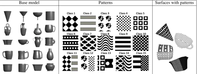
Base model Patterns Surfaces with patterns
Fig. 7. The 20 base models used in the SHREC’18 benchmark are shown on the left. Each pattern (middle) was applied to all of the base models and changed in terms of their luminosity (examples of the final models are shown on the right).
GRAVITATE(geo) GRAVITATE(col)
Feathered Pattern of Spirals Pattern Circlets
Line Smooth Hatched Pattern Fringe Fringe
Guilloche Six Petals Chequer Striped Band Pattern of circlets (P.o.C) (Painted)
Lotus and Buds Scales v1 Scales v2 Guilloche v2 Pattern of Curves
Fig. 8. One sample per each class of the GRAVITATE datasets. Class labels are given by experts of the field [4].
(a) (b)
Fig. 9. Visual representation of how the height-field is computed. Starting from a point P, the plane of linear regression is computed (a) and a scalar value hf is assigned each point Pjin the neighborhood of P (b). The area
represented in (b) is the same as the light blue one on (a), with only Pj
represented here for the sake of clearness.
value is negative if −→nP·
−−→
PiP< 0, where −→nPis the normal of the
1
point P. A point common to the neighborhoods of two different
2
points may have different height values with respect to the two
3
neighborhood regression planes. Figure 9 shows how the HF is
4
computed.
5
For colorimetric patterns, only the CIELab color-space [42,
6
43] is considered (the L-channel in particular, which encodes
7
the luminosity of the colors).
8
5. Experimental results and discussions 9
This Section summarizes the mpLB performances over the 10
different datasets with the different settings described in Sec- 11
tion 5.1. Then, in Section 5.2 we analyze the robustness of the 12
mpLBP descriptor to surface noise, different bendings a pat- 13
tern may be embedded in and different neighborhood sampling 14
schema. Finally, Section 5.4 shows the timing comparisons be- 15
tween the mpLBP and the edgeLBP. 16
5.1. Experimental results 17
Before discussing the results, it is worth noticing that the 18
evaluation scores of the mpLBP reported in this paper are 19
slightly different than those in [12]: a regression plane align- 20
ment bug was found in our previous implementation and it is 21
now corrected. 22
Performances on the SHREC’17 benchmark. In addition to the 23
methods of [3] that obtained the best performances, we com- 24
pare the mpLBP with the edgeLBP [10] and the SIFT-based 25
method in [13]. Among all the settings tested, the best per- 26
mpLBP - Cmax 0.933 0.706 0.845 0.744 0.449 0.871 mpLBP - Cmin 0.922 0.732 0.861 0.738 0.442 0.862 mpLBP - Cmean 0.911 0.733 0.861 0.763 0.447 0.888 mpLBP - Cmean* 0.917 0.733 0.863 0.761 0.427 0.875 mpLBP - Cmean* 0.922 0.728 0.862 0.763 0.426 0.877 mpLBP - Cgauss 0.939 0.707 0.845 0.744 0.483 0.872 mpLBP - SI 0.911 0.729 0.835 0.749 0.440 0.876 mpLBP - HF 0.672 0.353 0.451 0.431 0.281 0.658 Complete Dataset
Method NN 1-Tier 2-Tier mAP e nDCG CMC-2 0.763 0.272 0.389 0.271 0.261 0.686 KLBO-FV-IWKS 0.986 0.333 0.449 0.339 0.332 0.759 edgeLBP - run2 0.986 0.634 0.780 0.669 0.421 0.902 T/mC/SIFT/FV 0.993 0.712 0.850 0.739 0.647 0.929 mpLBP - Cmax 0.994 0.678 0.820 0.738 0.653 0.931 mpLBP - Cmin 0.997 0.677 0.815 0.733 0.653 0.931 mpLBP - Cmean 0.994 0.702 0.841 0.759 0.665 0.938 mpLBP - Cgauss 0.994 0.678 0.820 0.738 0.653 0.931 mpLBP - SI 0.997 0.688 0.813 0.737 0.650 0.930 mpLBP - HF 0.999 0.383 0.480 0.431 0.419 0.802
Table 1. Results on the SHREC’17 benchmark, both the Original (Top) and the Complete (Bottom) Dataset. Runs marked with ∗ are those which point neighborhood are rotated by a random angle around the normal of the respective point.
of the models in the dataset have a low number of vertices, we
1
resampled them to 40000 vertices using the Remesh tool [44].
2
Table 1 reports the mpLBP scores together and compares them
3
with the other methods, with respect to NN, FT, ST, e-measure,
4
mAP and nDCG. In this table we also include the results
ob-5
tained when testing the independence from the cut of the grid
6
on the neighborhood of the points. We mark with ∗ the runs
7
to which we added to each point neighborhood a small rotation
8
of the tangent parametrization around the point normal (from
9
0 to 2π). The results show that adding this rotation does not
10
influence critically the results of our method.
11
The mpLBP scores equivalently or slightly better than the
12
edgeLBP and T/mC/SIFT/FV over the SHREC’17 benchmark
13
on geometric patterns, with small variations depending on the
14
surface property chosen. Overall, over this benchmark, the
15
mpLBP performs well with all the curvature-based properties;
16
in particular, the mean curvature provides slightly better
re-17
trieval performances. However, the NN performance over the
18
complete dataset of mpLBP with the height field highlights how
19
this property is able to characterize a model and its re-samplings
20
but it less robust to different surface bendings.
21
Performances on the SHREC’18 benchmark. The performance
22
of mpLBP on this benchmark is compared against those
ob-23
tained in [15] and [11]. The parameters settings with the best
24
evaluations are R = 0.10 nrad = 7 multP = 1 (set1) and
25
R = 0.14 nrad = 7 multP = 1 (set2). Table 2 summarizes
26
the best scores obtained (more runs and methods are available
27
in [15] and [11]).
28
Over this benchmark, mpLBP and edgeLBP perform
equiv-29
alently, even if the time for evaluating the edgeLBP on this
30
dataset is approximately twenty times higher than the mpLBP
31
(details on the computation costs are provided in Section 5.4).
32 mpLBP - set1 0.965 0.739 0.862 0.781 0.600 0.910 mpLBP - set2 0.960 0.744 0.864 0.762 0.590 0.900 Complete Dataset Run NN FT ST maP e nDCG TWB3 0.593 0.417 0.564 0.460 0.376 0.711 V2 0.79 0.433 0.594 0.493 0.39 0.753 edgeLBP-R4 0.903 0.673 0.827 0.722 0.557 0.878 edgeLBP-R5 0.923 0.667 0.805 0.727 0.546 0.878 mpLBP - set1 0.903 0.739 0.862 0.668 0.520 0.850 mpLBP - set2 0.907 0.573 0.735 0.639 0.510 0.840
Table 2. Performance scores over the Single pattern dataset and Complete dataset of the SHREC’18 benchmark.
Indeed, to guarantee the decorations were intelligible, the orig- 33
inal surfaces were densely sampled (100K vertices, each) and 34
this corresponds to a demanding task for the edgeLBP. On the 35
contrary, this is a good basis for mpLBP because the key issue 36
for its success is that the point cloud is dense enough, i.e., most 37
of the sectors of the descriptors should not be empty. 38
Performances on the GRAVITATE dataset. We run the mpLBP 39
on both datasets with 4 different settings. The results are com- 40
pared with those reported in [4] for edgeLBP on the GRAVI- 41
TATE datasets. In particular, on GRAVITATE(geo) we used the 42
Shape Index as h function, as it is done in [4]. In Table 3, the 43
best mpLBP run we had is compared to the edgeLBP results. 44
As a general premise, since the dataset classes contain few 45
models (less than 10), even a variation of 0.1 in the scores 46
means that only one model is miss-classified. The performances 47
of the edgeLBP and mpLBP are comparable, with differences 48
that depend on the type of pattern and the quality of the model. 49
This can be observed by the overall performances of the runs. 50
Looking at the single class performances, the NN measures are 51
almost identical, with the edgeLBP being slightly more efficient 52
on the geometric patterns. The opposite is true on the colori- 53
metric ones, where the patterns are more degraded. This may 54
be explained by the fact that since the mpLBP scouts an en- 55
tire area for each sampling (sector) rather than a single point 56
to code the evolution of the ring properties, it slightly averages 57
the local surface properties simulating a slight smoothing effect. 58
This can be positive in case of noisy colorimetric patterns but 59
it could lead to a confusion between geometric noise and actual 60
small surface variations. 61
5.2. Robustness of the descriptor 62
In [12] we already explored the robustness of the mpLBP de- 63
scriptor to noise. In this work, we also analyzed the robustness 64
of the pattern descriptor of a fixed pattern when the latter lies 65
on surfaces with different bendings. All this robustness analysis 66
are reported in this Section. 67
Robustness to noise. The popularity of scanning devices that 68
can digitize objects increased the number of acquired 3D mod- 69
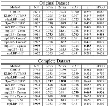
GRAVITATE(geo) results
edgeLBP settings: nrad= 7, N = 15, R = 0.6cm
Class considered NN FT ST e nDCG Feathered Pattern 1.000 0.722 0.911 0.434 0.934 Pattern of Circles 1.000 0.922 0.978 0.439 0.989 Spirals 1.000 0.644 0.756 0.385 0.911 Line Pattern 0.700 0.300 0.367 0.263 0.661 Smooth Fringe 1.000 0.467 0.500 0.229 0.804 Hatched Fringe 1.000 0.400 0.589 0.371 0.773 Overall 0.950 0.576 0.683 0.354 0.845
mpLBP settings: nrad= 5, multP = 4, R = 1cm
Class Label NN FT ST e nDCG Feathered Pattern 1.000 0.511 0.767 0.410 0.849 Pattern of Circles 1.000 0.889 0.944 0.439 0.976 Spirals 1.000 0.544 0.700 0.400 0.870 Line Pattern 0.800 0.289 0.444 0.302 0.685 Smooth Fringe 1.000 0.522 0.533 0.239 0.818 Hatched Fringe 1.000 0.400 0.500 0.366 0.765 Overall 0.967 0.526 0.648 0.359 0.827 GRAVITATE(col) results
edgeLBP settings: nrad= 5, P = 15, R = 0.5cm
Class Label NN FT ST e nDCG Guilloche v1 1.000 1.000 1.000 0.171 1.000 Six Petals 0.500 0.500 0.767 0.270 0.720 Chequer 0.857 0.571 0.738 0.271 0.811 Striped band 0.800 0.200 0.400 0.222 0.544 P.o.C. (Painted) 1.000 1.000 1.000 0.171 1.000 Lotus and Bud 0.500 0.333 0.583 0.171 0.666 Scales v1 0.429 0.310 0.619 0.316 0.579 Scales v2 1.000 1.000 1.000 0.171 1.000 Guilloche v2 1.000 1.000 1.000 0.171 1.000 Pattern of Curves 0.500 0.250 0.250 0.086 0.424 Overall 0.735 0.582 0.723 0.217 0.758 mpLBP settings: nrad= 7, P = 15, R = 0.5cm Class Label NN FT ST e nDCG Guilloche v1 1.000 1.000 1.000 0.171 1.000 Six Petals 0.500 0.400 0.767 0.270 0.709 Chequer 1.000 0.714 0.976 0.316 0.924 Striped band 0.600 0.250 0.500 0.189 0.567 P.o.C. (Painted) 1.000 1.000 1.000 0.171 1.000 Lotus and Bud 0.500 0.417 0.583 0.143 0.566 Scales v1 0.571 0.357 0.643 0.263 0.680 Scales v2 0.750 0.333 0.667 0.171 0.673 Guilloche v2 1.000 1.000 1.000 0.171 1.000 Pattern of Curves 0.500 0.167 0.250 0.100 0.427 Overall 0.742 0.693 0.918 0.211 0.755
Table 3. Results on the GRAVITATE datasets, and comparison with those of the edgeLBP.
acquired data can be corrupted by acquisition noise.
Further-1
more, objects can be degraded by time or other factors, which
2
can lead to corruption of the patterns that lie on the surface of
3
the object.
4
Noise in general is an unwanted variation of a signal (the
5
surface, in this case) usually of small scale. Patterns also are
6
usually small, thus the noise is a problem that is worth
address-7
ing. We added noise with various amplitudes to some of our
8
test models. Such variations change the h function and as a
9
consequence the whole punctual descriptor. Depending on the
10
pattern nature, we considered different noise addition. The
ge-11
ometrical patterns are corrupted with a Gaussian noise on the
12
vertices, based on a parameter λg, expressed as a percentage of
13
the diameter of the smallest bounding sphere. The values of λg
14
considered are 0.2 and 0.4. See Figure 10 (Top) for an example
15
of mesh degradation.
16
Colorimetric patterns are instead corrupted by adding small
17
variations to the RGB values stored on the model vertices. Such
18
variation is bounded to the parameter λc, an integer value added
19
to each RGB channel (we assume the three channels to range
20
from 0 to 255). For example, λc= 5 added three random offsets
21
in the interval [−5,+5] to each color channel. In our tests, we
22
used λc∈ {5, 7} (see Figure 10 (Bottom)).
23
The noise tests are run on the SHREC’17 Original dataset
24
for the geometric patterns and on the SHREC’18 Single pattern
25
dataset for the colorimetric one. Results are reported in
Ta-26
ble 4. We observe that the performances significantly decrease
27
in presence of heavy noises, while the mpLBP is robust in case
28
of lighter ones. We think that this behaviour derives from the
29
strategy we adopt to evaluate a property in the sectors. Indeed,
30
the use of the weighted mean for each sector balances the small
31
variations of the h function, while it starts being less efficient
32
in case of higher variations (in this case, all the sectors become
33
similar).
34
λg= 0 λg= 0.2 λg= O.4
λc= 0 λc= 5 λc= 7
Fig. 10. Pattern distortion when noise is randomly added. Top row: a geo-metric pattern is corrupted using increasing Gaussian noise. Bottom row, an increasing random noise is added to each RGB color channel.
SHREC’17: Original Dataset, geometric noise
Method NN 1-Tier 2-Tier mAP e nDCG mpLBP - set1 Clean 0.917 0.711 0.859 0.743 0.420 0.861 mpLBP - set1, λg= 0.2 0.911 0.693 0.846 0.733 0.380 0.790
mpLBP - set1, λg= 0.4 0.872 0.618 0.769 0.664 0.350 0.753
SHREC’18: Single Pattern Dataset, colorimetric noise
Method NN 1-Tier 2-Tier mAP e nDCG mpLBP - set1 Clean 0.965 0.739 0.862 0.781 0.600 0.910 mpLBP - set1, λc= 5 0.915 0.514 0.653 0.586 0.440 0.822
mpLBP - set1, λc= 7 0.75 0.332 0.445 0.457 0.355 0.741 Table 4. mpLBP performance for data corrupted with noise. Top: the Original Dataset of the SHREC’17 benchmark, Bottom: Single Pattern Dataset of the SHREC’18 benchmark.
Distances of each pattern descriptor of the bent surfaces from the same pattern embedded into a flat one
Bending 1 Bending2 Beinding3 Bending4 Circles 0.237 0.032 0.058 0.0794 Crosses 0.089 0.084 0.100 0.105
Fig. 11. Examples of two patterns embedded on surfaces with gradually stronger bendings. The table reports the distances between the pattern descriptor of the pattern embedded on the flat surface and on the bent surfaces. The L2norm is used to compute such distances.
Robustness to surface bendings. A very relevant feature of a
1
pattern descriptor on surfaces is its robustness to different
bend-2
ings of the underlying surface. To test this, we created a pattern
3
of circlets and applied it to surfaces with more and more severe
4
bendings. These models are reported in Figure 11 (First row).
5
Since they are generated from a synthetic surface and adopting
6
an isotropic bending we are guaranteed that the models possess
7
the same pattern. In the second row of Figure 11, the
corre-8
sponding descriptors are showed. A similar test is done using
9
a pattern made up by small crosses (see Figure 11 - Third and
10
Fourth rows). From the results, one can observe that the pattern
11
descriptor changes depending on the embedded pattern.
More-12
over, it remains quite close, although not perfectly identical, for
13
the same pattern across the bending changes. This show that
14
the descriptor is more sensible to changes in the patterns it
de-15
scribes and far less sensitive to the surface bending.
16
Robustness to different model samplings. In the experiments
17
shown in Section 5.1, the models with a low resolution were
18
re-sampled, increasing the vertex density to reach a reasonably
19
dense representation. Therefore, it is worth exploring the
be-20
haviour of the pattern descriptor when it is computed for di
ffer-21
ent sampling density of the same model. We used the SHREC17
22
Original Dataset for this experiment. We selected two of the
23
models of this dataset (one from class 8 and one from class 12)
24
and down-sampled it from 40000 vertices to 3000 vertices, with
25
various steps, using the default sampling scheme implemented
26
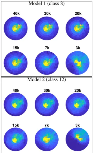
in [44]. Figure 12 shows the pattern descriptor computed. It
27
is easy to notice that the pattern descriptor holds its shape and
28
changes when the number of vertices considerably decreases
29
(although in the examples 7000 is still sufficiently stable with
30
respect to the higher samplings we noticed that around 10000
31
vertices is a good quality compromise). This test shows that it
32
Model 2 (class 12)
Fig. 12. Pattern descriptor robustness to different samplings. The number of vertices of the model is on top of the respective pattern descriptor.
is possible to have similar performances when re-sampling with 33
different vertex resolutions, but it is necessary to have a mini- 34
mum vertex density in order to have more stable pattern de- 35
scriptors (in this case, approximately 10000 vertices or more). 36
Robustness to different choices of the parameters. The choice 37
of the mpLBP parameters (R, nradand multP) is crucial for the 38
performance of the method because they are related strictly re- 39
lated at the resolution a pattern is analysed. Anyway, we noticed 40
that the performance of the mpLBP is quite stable for small 41
variations of the parameters. In other words, slightly chang- 42
ing the parameters (all three of them) will not jeopardise the 43
performances of the method. This fact was experimentally con- 44
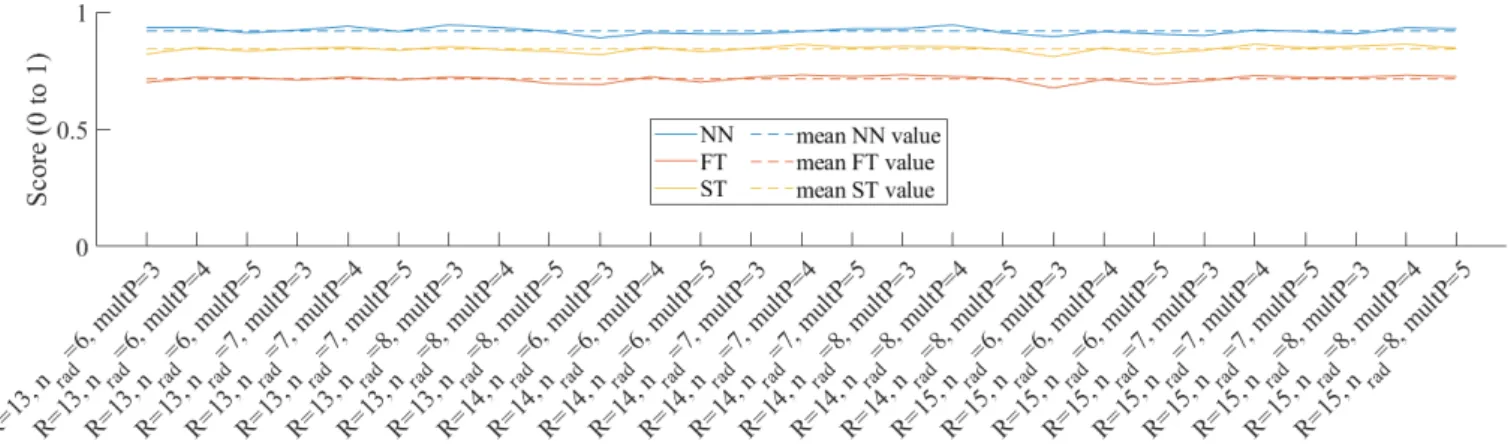
firmed by selecting 27 variations of the best mpLBP run over 45
the SHREC17 original dataset (see Table 1). The performance 46
in terms of NN, FT and ST scores of the mpLBP are reported 47
in Figure 13 for all these 27 settings. On the horizontal axis we 48
report the parameter setting, while the vertical axis represents 49
the performance score (different colours are used for the NN, 50
FT and ST, respectively). The performances are very similar 51
for all the settings. The maximum discrepancy observed across 52
all the evaluation measures is around 0.05, which is very tiny, 53
Fig. 13. The performances of 27 different mpLBP runs on the SHREC17 dataset, with different parameter settings. The dashed lines represent the mean value of the respective evaluation measure.
5.3. Different choices of the ring sampling scheme
1
We took the four possible variants of the point neighborhood
2
sampling schemes described in Section 3.3 and we evaluated
3
them on the SHREC’17 Original dataset. As shape
proper-4
ties, we considered the height-field as defined in Section 4.3
5
because of its simplicity and rough shape description and the
6
Mean curvature because it generally performs well over
geo-7
metric patterns. With reference to the labels defined in Section
8
3.3, Scheme 1 is computed using R ranging from 7 to 15 and
9
pxres ranging from 10 to 16. To evaluate Schemes 2, 3 and
10
4 we extracted the standard punctual descriptor with
parame-11
ters R = 14, nrad = 7 and multP = 4 and we considered only
12
the sectors highlighted in the schemes. In this Section, we
re-13
port only the most significant runs. Table 5 summarizes the
14
results of the tests of mpLBP with these settings. In
particu-15
lar, when using sampling scheme 1 with h equal to the Mean
16
Curvature, we use R= 10 and pxres = 16, while when using
17
sampling scheme 1 with h= HF, we set R = 7 and pxres = 12.
18
Note that the size of the mpLBP descriptor varies according
19
to the different neighborhood sampling schemes. Looking at
20
the retrieval performances, we notice that mpLBP with scheme
21
1 (with a square-based point neighborhood) performs poorly
22
compared to the other schemes. This is not really surprising
23
because a square-like point neighborhood inserts an orientation
24
and an anisotropic sampling of the model. Unlike images where
25
a square-like neighborhood is compliant with the intrinsic grid
26
structure, for a surface, a circle or a geodesic neighborhood
bet-27
ter reflect the intrinsic surface metric. Schemes 2 and 3
high-28
light that other sampling strategies over a circular neighborhood
29
are possible and lead to good performances. On the contrary a
30
too sparse sampling like the one proposed the Scheme 4
jeopar-31
dises the mpLBP performance. These results highlight that the
32
mpLBP technique can be adapted to different schemes and that
33
it is possible to keep limited the size of the descriptor compared
34
to the original mpLBP settings [12] that probably generated a
35
descriptor with redundant information.
36
5.4. Computational time
37
The mpLBP algorithm is implemented in around 200
MAT-38
LAB lines of code. The most expensive part, in terms of
com-39
putational cost is the creation of the punctual descriptor, which
40
SHREC’17: Original Dataset, scheme variants
Parameters NN 1-Tier 2-Tier mAP e nDCG Scheme 1 - Mean C. 0.739 0.395 0.534 0.481 0.324 0.705 Scheme 1 - HF 0.794 0.504 0.622 0.560 0.360 0.755 Scheme 2 - Mean C. 0.928 0.707 0.835 0.746 0.447 0.878 Scheme 3 - Mean C. 0.928 0.667 0.804 0.715 0.436 0.861 Scheme 4 - Mean C. 0.856 0.596 0.745 0.658 0.418 0.813
Table 5. Retrieval results of the various sampling schemes on the SHREC’17 Original Dataset.
is based on a kd-tree. This characteristic allows the mpLBP 41
algorithm to run in a much shorter time if compared, for exam- 42
ple, with the edgeLBP, while keeping similarly high evaluation 43
scores. By running both edgeLBP and mpLBP on meshes with 44
different number of vertices (from 5000 gradually to 120000 45
vertices) and different parameter settings, we can see the huge 46
gap between the timings of the two methods (see Table 6). 47
Tests are run on a personal computer Intel Core i7 processor 48
(at 4.2 GHz) with 32Gb RAM. The edgeLBP (as currently im- 49
plemented) has the number of sectors per ring constant across 50
all the rings. In order to have a fair comparison, we also set the 51
number of sectors to be constant for mpLBP (i.e., Pj= P with 52
P ∈ N fixed). We observed that nradand P do not affect the com- 53
putation times that much. Indeed, the radius size and the num- 54
ber of vertices are the biggest bottlenecks. Figure 14 provides 55
another computational time comparison between edgeLBP and 56
mpLBP showing the much more sever increase of the edgeLBP 57
computational cost compared to the cost increase of the mpLBP. 58
These timings are those obtained on the 120k vertices mesh, 59
with R= 4.5, nrad= 4 P = 15. We do not report the same trend 60
representation for other mesh and parameters for brevity rea- 61
sons, but those trends are almost identical to the ones reported 62
(only the time scale (y-axis scale) changes based on the radius). 63
6. Discussions and concluding remarks 64
We extended the LBP concept to surfaces represented as 65
point clouds and defined a novel description, called mpLBP. 66
Such a descriptor is able to keep state of the art performance and 67
run more efficiently than its analogous edgeLBP which is based 68
on a surface tessellation, see Section 5.4. Overall, the mpLBP 69
Fig. 14. Computational time trends for the mpLBP and edgeLBP. 5K R=2,5 R=3,5 R=4,5 nrad= 4, P = 12 22.04/2.88 16.89/1.38 19.06/1.35 nrad= 7, P = 12 15.74/1.59 19.91/1.55 24.54/1.60 nrad= 4, P = 18 11.40/1.27 15.89/1.48 17.12/1.38 nrad= 7, P = 18 16.14/1.95 20.39/1.88 30.18/2.55 10K R=2,5 R=3,5 R=4,5 nrad= 4, P = 12 59.33/4.23 79.09/4.62 92.31/5.09 nrad= 7, P = 12 71.69/4.35 95.58/4.93 116.51/5.46 nrad= 4, P = 18 52.92/3.95 76.55/4.77 83.54/4.95 nrad= 7, P = 18 72.43/5.01 95.86/5.53 140.23/6.25 15K R=2,5 R=3,5 R=4,5 nrad= 4, P = 12 81.13/5.31 118.42/7.48 143.29/8.00 nrad= 7, P = 12 107.26/6.63 143.08/7.52 178.01/8.40 nrad= 4, P = 18 81.92/5.96 115.85/7.38 128.10/7.49 nrad= 7, P = 18 107.83/7.53 143.77/8.19 188.56/9.32 30K R=2,5 R=3,5 R=4,5 nrad= 4, P = 12 341.81/19.90 516.53/28.52 651.99/33.08 nrad= 7, P = 12 454.23/23.30 618.36/28.36 805.07/33.72 nrad= 4, P = 18 348.93/20.43 507.31/28.21 583.39/30.31 nrad= 7, P = 18 456.26/25.10 621.50/29.75 811.99/35.25 90K R=2,5 R=3,5 R=4,5 nrad= 4, P = 12 2378.79/109.32 3661.28/158.43 4344.93/196.08 nrad= 7, P = 12 3024.61/122.58 4142.54/157.74 5200.46/194.75 nrad= 4, P = 18 2344.02/110.05 3481.22/160.97 3989.87/179.15 nrad= 7, P = 18 3034.85/128.34 4145.79/163.19 5704.31/201.03 120K R=2,5 R=3,5 R=4,5 nrad= 4, P = 12 4314.18/165.65 6612.18/260.30 8341.62/335.82 nrad= 7, P = 12 5583.24/189.33 7812.26/260.18 9954.04/332.90 nrad= 4, P = 18 4236.92/170.22 6586.75/262.25 7626.82/309.25 nrad= 7, P = 18 5596.74/198.12 7806.80/266.27 10438.45/348.40 Table 6. Computational times for edgeLBP and mpLBP (in seconds). The top-left cell of each table indicates the number of vertices.
Indeed, in presence of a small noise intensity that simulates the 5
possible perturbation of a common scanning device, the perfor- 6
mances are competitive with the current state of art methods. 7
Moreover, it is robust to different surface bendings and is able 8
to support different sampling schemes, as discussed in Section 9
5.3. 10
Other competing methods such as the T/mC/SIFT/FV 11
method in [13] implicitly assumes that the same geodesic 12
‘sphere’ centered in every patch is able to parameterize all the 13
models. The sphere radius is unique and can be obtained eas- 14
ily for the SHREC’17 dataset because the patches have com- 15
parable size but it is hard to obtain on datasets with models of 16
different size. Moreover, such a single patch parameterization 17
approach is not suitable to deal with datasets containing models 18
with handles and protrusions, like some of SHREC’18 dataset. 19
Indeed, T/mC/SIFT/FV translates the problem into a texture im- 20
age comparison and requires a resampling with 20K vertices, 21
while mpLBP works directly on the 3D model (mesh or point 22
cloud). From these considerations, T/mC/SIFT/FV can be un- 23
derstood as a global descriptor that down-samples the model 24
vertices as a pre-processing step. On the contrary, the mpLBP 25
descriptor is local and its computation depends on the number 26
of vertices, therefore the time complexities are not directly com- 27
parable, while also scoring similar performances. 28
While most patterns considered in this work are well de- 29
scribed by a single scalar function for each point of the model, 30
the possibility of describing patterns based on two or more 31
properties (e.g.: curvature plus color, multiple color channel 32
and so on) is of interest and one of the future research paths. Fu- 33
ture reasoning will be devoted to the punctual descriptor used 34
by the mpLBP. Since its resolution can easily be customized 35
and it is not tied to a specific surface property (curvatures, col- 36
ors, height-fields and so on), the punctual descriptor itself could 37
be used as a feature vector to encode different surface details 38
and/or as the starting point for more advanced local descrip- 39
tions. A further extension is the application of the punctual 40
descriptor to the problem of pattern recognition over surfaces. 41
This last is still an open problem, as observed in [5], and a quick 42
and well performing technique such as the mpLBP is a promis- 43
ing contribution towards a possible solution. 44
7. Acknowledgments 45
This study was partially supported by the CNR-IMATI 46
projects DIT.AD004.028.001 and DIT.AD021.080.001, and the 47
e-Roma project from the Agence Nationale de la Recherche 48
(ANR-16-CE38-0009). 49
References 50
[1] Othmani, A, Voon, LFLY, Stolz, C, Piboule, A. Single tree species clas- 51 sification from terrestrial laser scanning data for forest inventory. Pattern 52 Recognition Letters 2013;34(16):2144–2150. 53
![Fig. 2. A mpLBP descriptor at point p ˜ (marked with a light-blue star in (a)). (b): neighborhood S [ ˜ p] of p ˜ is shown with a dark sphere](https://thumb-eu.123doks.com/thumbv2/123doknet/14502303.528062/5.892.88.822.98.198/mplbp-descriptor-point-marked-light-neighborhood-shown-sphere.webp)