Control system failure monitoring using generalized parity relations

Accepted by:

Professor Wallace E. Vander Velde Thesis Supervisor Department of Aeronautics and Astronautics

. ,.

rofessor Harold Y. Wachman Chairman, Department Graduate Committee MASSACHUSETTS "'STIi UTE

OF TECHNOLOGY

FEB 19 1991

1 UBRARIES

Aero

Control System Failure Monitoring Using

Generalized Parity Relations

by

Christiaan Mauritz Van Schalkwyk

MIng (Elektron) Universiteit van Pretoria (1987)

BIng (Elektron) Universiteit van Pretoria (1980)

Submitted to the Department of Aeronautics and Astronautics

in partial fulfillment of the requirements for the degree of

Master of Science in Aeronautics and Astronautics

at the

Massachusetts Institute of Technology

February 1991

SMassachusetts

Institute of Technology 1991

Signature of Author:

Department of Aeronauet' and Astronautics

December 14, 1990

Control System Failure Monitoring Using

Generalized Parity Relations

by

Christiaan Mauritz Van Schalkwyk

Submitted to the Department of Aeronautics and Astronautics in partial fulfillment of the requirements for the degree of

Master of Science in Aeronautics and Astronautics at the Massachusetts Institute of Technology

Abstract

Many applications require that a control system must be tolerant to the failure of its com-ponents. This is especially true for large space-based systems that must work unattended and with long periods between maintenance. Fault tolerance can be obtained by detect-ing the failure of the control system component, determindetect-ing which component has failed, and reconfiguring the system so that the failed component is isolated from the controller. This work reports on component failure detection experiments that were conducted on an experimental space structure, the NASA Langley Mini-Mast.

Two methodologies for failure detection and isolation (FDI) exist that do not require the specification of failure modes and are applicable to both actuators and sensors. These methods are known as the Failure Detection Filter and the method of Generalized Parity Relations. The latter method was applied to three different sensors types on the Mini-Mast. Failures were simulated in input-output data that was recorded during operation of the Mini-Mast. Both single and double sensor parity relations were tested and the effect of several design parameters on the performance of these relations is discussed. The detection of actuator failures is also treated. It is shown that in all the cases it is possible to identify

the parity relations directly from input-output data. Frequency domain analysis is used to explain the behaviour of the parity relations.

Thesis leader: Prof. Wallace E. Vander Velde

Title: Professor of Aeronautics and Astronautics Massachusetts Institute of Technology

Acknowledgement

I would like to thank my thesis leader, Prof. Wallace E. Vander Velde, for his guidance and many interesting discussions during the course of this work.

Sincere thanks to Messrs. Johann Ahlers and Coen Bester who made all of this possible. Specifically I would like to thank Mr. Johann Ahlers whose division at the CSIR, Mikomtek, financed a great part of the studies.

Special thanks to my mother and sisters for their support. I truly appreciate all the things that they have done during the last three years.

To my friends back home, thanks for your encouragement, support, performing various tasks, general stationkeeping, ... , and for being friends; in reverse alphabetical order: Thys & Christa, Thea, Marion, Marianne, Johann, CT, Carin, die Britse. The list should be much longer. To everybody else, my sincere thanks and I apologize for omitting your name.

Several people made my stay in the USA bearable and I would like to thank them here. Again in reverse alphabetical order: Riaan & Cecilia, Heron & Petra, Fred & Melanie (they deserve a standing ovation), Fanie & Gerda, Daniel & Mattie.

A word of appreciation goes to my fellow students Riaan, Norman, Mathieu, John (I hope you find a squash court near JPL), for suggestions, reading copies of my thesis, coffee breaks, lunch, squash games, ....

This work was supported by NASA Research Grant NAG-1-968 under the Controls/Struc-tures Interaction program.

2 Generalized Parity Relations

2.1 Single Sensor Parity Relations ... 2.2 Double Sensor Parity Relations ... 2.3 Actuator Parity Relations ... 2.4 Example ...

Contents

Abstract Acknowledgement List of Figures Notation Symbols 1 Introduction

3 Displacement Sensor Failure Detection 35

3.1 Introduction .... ... . ... . 35

3.2 Model-based Single Sensor Parity Relations . . . ... .. 41

3.3 Identified Single Sensor Parity Relations .. . . . . . . . . . .... . 47

3.4 Transfer functions of model-based and identified Single Sensor Par-ity Relations ... . ... 51

3.5 Increased Sampling Period .. ... ... .. 55

3.6 Double Sensor Parity Relations . .... . . . . . . . . . . 57

3.7 Sum m ary ... . . . ... ... 68

4 Accelerometer and Gyro Failure Detection 70 4.1 Introduction ... ... . .. . .. ... .. 70

4.2 Single Sensor Parity Relations ... . . . . . . . ..... 74

4.3 Double Sensor Parity Relations . . . ... ... 79

4.4 Sum m ary ... ... . . . ... 87

5 Actuator Failure Detection 88

6 Conclusion 96

A Second order system analysis 101

B Mini-Mast state-space model 103

3.1 3.2 3.3 3.4 3.5 3.6 3.7 3.8

Schematic diagram of the Mini-Mast. . . Spectrum of input signal . . . . Spectrum of Displacement Sensor 2 . . .

Displacement Sensor D1 failure . . . . . Components rl,y and rl,, of SSPR r, . .

Displacement Sensor D3 failures . . . .

Noisy sensor ...

Identified SSPR residual r3 . . . . . . .

List of Figures

1.1 FDI block diagram ...

2.1 Block diagram of SSPR Residual Generator . . . . 2.2 Block diagram of DSPR Residual Generator . . . .... 2.3 Block diagram of SAPR Residual Generator . . . ..

2.4 Block diagram of the plant and SSPR Residual Generator . . .

2.5 Transfer functions of the SSPR Residual Generator . . . ..

. 36 . 39 . 40 . 42 . 43 . . .. . . . . . . . . 4 5 .. . . . .. . . . . 4 6 . . . . . 4 7 . . . . . 23 . . . . . 25 . . . . . 29 . . . . . 32 . . . . . 33

esidual r3 . . . . . . . . . . 4 9 .... . . . 5 0 cations . ... . . . . . . . . ... . 52 r functions . . . . . . . ... 53 .... . . . 5 4 . . . . 5 5 .... . . . 5 6 tor transfer functions IT, and 2T, . . .. . . 57

and r13 .. .. . . . . . . . . . . . .. . . 59 and r13 . . . .. . . . . . . . . .. . . 60 i r3 2 . . . . . . . . . .. . .

61

21 and r23 .. . . . . . . . .. . . .. 62

1

r23 . . . . .

64

1 r2 3, 20 lags . . . . 65 and r13, 10 lags, 2T . . . . . 66

1

r23, 20 lags, 2T

.

.

. . . .

. . . 67

on, u = filtered white noise . . . . 71

on, u = 4T, white noise . . . . 72

Model-based SAPR for X-wheel failure . . . . . Identified SAPR for X-wheel failure . . . . SAPR residual for Y-torque wheel failure. . . . SAPR residual for Y-torque wheel failure, noisy

. ... . ... 89

...

...

89

. . . . 89

. . . . 9 1 measurement . . . . 92

SAPR residual contributions for Y-torque wheel failure, noisy measurement SAPR Residual Generator transfer functions ... 4.4 4.5 4.6 4.7 4.8 4.9 4.10 4.11 4.12 4.13 4.14 4.15 4.16 4.17 5.1 5.2 5.3 5.4 Experimental setup ... ... ... . 74

SSPR for Y-axis accelerometer failure, 20 lags, IT . . . . . .. 75

SSPR for Z-axis gyro failure, 20 lags, IT .. . . . . . . . . . . . 75

SSPR for Y-axis accelerometer failure, 20 lags, 1T,; filtered residual ... .. 76

SSPR for Z-axis gyro failure, 20 lags, IT,; filtered residual . . . . 76

SSPR for Y-axis accelerometer failure, 20 lags, 2T . . . . . . . . . . 77

SSPR for Z-axis gyro failure, 20 lags, 2T .... . . . . . . . . ... . 77

DSPR for X-axis accelerometer failure, (11,10) lags, lT . . . .. 80

DSPR for Z-axis gyro failure, (11,10) lags, 1T . . . . . .. 81

DSPR for X-axis accelerometer failure, (11,10) lags, 2T, . . . .. 82

DSPR for Z-axis gyro failure, (11,10) lags, 2T . . . . . . . . .... 83

DSPR for X-axis accelerometer failure, (11,10) lags, 2T . . . .. 84

SSPR for Z-axis gyro failure, 20 lags, 1T ... . . . . . . . .... 86

Notation

Vector notation

Vectors will be written as a single column and will be denoted by bold lowercase characters. We will also use the Matlab notation where a column vector is written on one line and a semicolon is used to delimit the elements of the vector:

xG1E J ' x = (0.1)

Xn

= [xl; ... ; xn]. (0.2)

Row vectors will be written on one line and a comma will be used to delimit the elements of the vector:

x' c Rxn X '- = [I₁, ... , Xn]. (0.3)

A few special vectors, which will be defined explicitly, will be written with reversed indices:

,= E R'+'

3 = [)I;

.

; Oo].

(0.4)

Matrix notation

Bold uppercase letters will be used to denote matrices, the corresponding lowercase letters

with subscripts ij will be used to denote the (i,j) entry:

all • • aln

A E

Rmxn A= " aij E R. (0.5) ami . " amn

Columns of the matrix will be denoted by the vectors al, ... , an, and the rows will be denoted by the row vectors a', ... , a'm. The transpose of the matrix will be written as AT.

Symbols

ai parity relation coefficients, Equations (2.23) and (2.54)

c ₂ij parity relation coefficients, Equations (2.36)

A discrete-time state transition matrix, Equation (2.8)

A, continuous-time system matrix, Equation (2.5)

)3 parity relation coefficients, Equations (2.18) and (2.58)

B discrete-time input matrix, Equation (2.8)

B, continuous-time input matrix, Equation (2.5)

C output matrix, Equation (2.9)

cý ith row of C

Ci Equation (2.16) Cj Equation (2.32)

Ci Equation (2.52)

D feedforward matrix, Equation (2.9)

dý ithrow of D

DI Equation (2.17)

Dij3 Equation (2.33)

Di Equation (2.53)

ni Equations (2.12), (2.28), (2.40)

nJ Equation (2.28) R field of real numbers

ri(k) ith SSPR or SAPR residual, Equations (2.21), (2.56)

rij(k) ijth DSPR or DAPR residual, Equation (2.37) r3j(k) jith DSPR or DAPR residual, Equation (2.38)

T, sampling period

u(t) continuous-time input vector, Equation (2.5) u(k) discrete-time input vector, Equation (2.8)

ui(k) ith element of u(k)

u(ni) Equations (2.15) and (2.41)

ui(ni) Equation (2.50)

x(t) continuous-time state vector, Equation (2.5)

x(k) discrete-time state vector, Equation (2.8)

y(t) continuous-time measurement vector, Equation (2.6)

y(k) discrete-time measurement vector, Equation (2.9)

yi(k) ith element of y(k) y(ni) Equation (2.40)

y (ni) Equation (2.14)

Introduction

The requirement that a control system must be tolerant to the failure of its components and still perform safely and reliably puts stringent requirements on the reliability of the components that are used. Often the requirements on the reliability are so strict that it can only be achieved through some form of redundancy. An example is flexible space structures. Due to their large sizes and lightweight construction they have very low damping so that active control is necessary to do shape control and damp out vibrations throughout the structure. Active control is also necessary to perform other tasks like stationkeeping and attitude control. Systems in space must work for long unattended periods of time and with long intervals between maintenance so that a control system must be able to perform satisfactorily even when some of its components, especially the actuators and sensors, fail. To ensure stability of the control system and continue the mission it is necessary to detect the failure of a component. Once a failure has been detected and the failed component has been identified, the control system must be reconfigured to isolate the faulty component from the controller. Other examples of control systems that require very high reliability are

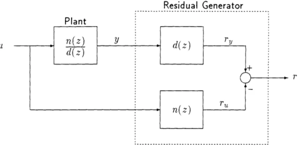
Figure 1.1: FDI block diagram.

aircraft engines, nuclear reactors, and process control systems, to name but a few.

To increase the reliability of a system some form of redundancy is usually used. Redundancy can be divided into two classes, hardware redundancy and analytical redundancy. In hard-ware redundancy the reliability is increased by replicating the control system components. A solution that is often applied is to use three or more sensors of the same kind to measure the same variable. A voting scheme is then employed to find the odd one out. Hardware redundancy has the advantage that it is insensitive to the magnitude of the failure and can detect any type of discrepancy. Although hardware redundancy is simple to implement, it is costly and adds unnecessary weight to the system. When many sensors and actuators are used it becomes impractical to triplicate each device. As an example, it is estimated that a large flexible space structure will have approximately 200 control system components. Tripling so many components is impractical and not cost effective. Another way to increase the reliability of a system is through analytical redundancy. Here the redundancy present in the model of the plant and input-output histories are used to detect and identify the failure of a component.

The typical form of a failure detection and isolation (FDI) system is shown in Figure 1.1. The FDI system is divided into two subsystems, the generation of residuals and decision

making, as shown in the figure. The Residual Generator uses the commanded inputs to the plant, the measured outputs from the plant, and a model of the plant to generate a set of residuals. The generation of residuals has been studied for many years and surveys of these methods can be found in Willsky [14], Basseville [1], and Merrill [12]. The Decision Function analyzes the residuals and based on this analysis makes a decision about the state of the actuators and sensors. Typical examples of this analysis are simple threshold detectors that compare the magnitudes of the residuals with a set of thresholds and declaring a failure when the amplitude exceeds the threshold. Other methods are moving average analysis and statistical decision theory. In the latter case a priori probabilities of the failure modes are hypothesized and it is possible to optimize for a specific mode of failure. It is not always possible to enumerate all modes of failure and obtain the corresponding probabilities. It is therefore desirable to have a methodology that does not require the specification of the failure modes and corresponding probabilities of failure. Also, the method should be applicable to both sensors and actuators. Only two methods satisfy the requirements set forth, the Failure Detection Filter by Beard [2] (see also Jones [6] and Massoumnia [10]) and the method of Generalized Parity Relations by Chow [4]. Because all analytical redundancy methods use a model of the plant they are all sensitive to modelling errors. The design of robust parity relations has been discussed by Lou et al. [8].

In this work we discuss the application of Generalized Parity Relations to an experimental flexible space structure, the NASA Langley Mini-Mast. We concentrated on the genera-tion of residuals and made no attempt to implement the Decision Funcgenera-tion. It should be clear from the examples that are presented in later chapters whether it would be possi-ble to detect the failure of a specific component. The thesis is structured as follows. In Chapter 2 we derive the equations for Generalized Parity Relations. Two special cases are treated: namely, Single Sensor Parity Relations (SSPR) and Double Sensor Parity Relations

(DSPR). Generalized Parity Relations for actuators are also derived. Chapter 3 describes the NASA Langley Mini-Mast and discusses the application of SSPR and DSPR to a set of displacement sensors located at the tip of the Mini-Mast. The performance of a reduced order model that includes the first five modes of the mast is compared to a set of parity relations that was identified on a set of input-output data. Both time domain and frequency domain comparisons are made. The effect of the sampling period and model order on the performance of the Residual Generators are also discussed. Chapter 4 presents failure de-tection experiments where the sensor set consisted of two gyros and an accelerometer. The effects of model order and sampling frequency are again illustrated. The detection of actu-ator failures are discussed in Chapter 5. Conclusions and directions for future research are given in Chapter 6.

Generalized Parity Relations

In the previous chapter we gave an outline of an FDI system where, for convenience of analysis, we divided the system into two functional parts: the Residual Generator and the Decision Function. In this chapter we give a brief description of a method to generate residuals. The method, known as Generalized Parity Relations, is treated in detail by

Chow [4] and Dutilloy [5].

There are two forms of analytical redundancy, namely direct redundancy and temporal redundancy. In direct redundancy a relation is formed by taking a linear combination of the instantaneous values of a set of sensors whose outputs are linearly dependent. As an example, let I denote a set of sensors whose instantaneous outputs are linearly dependent and let the jth sensor be a member of the set. We can then find a relation for the jth output yj :

yj(t)

=

Zaiyt(t).

(2.1)

iEI

i:Aj

Chapter 2

r(t) = yj (t) - E iy (t) (2.2)

iEf

i~j

which will be zero (except for noise or other unmodelled effects) when all the sensors are fully operational and nonzero in the case of a failure. Note that if r(t) is nonzero, any of the sensors in the set could have failed - this single relation does not indicate which sensor has failed.

In temporal redundancy, the histories of outputs and inputs are taken into account. The following example is used to illustrate temporal redundancy: consider a vehicle with mass

m and velocity v(t) with commanded force f(t) being applied to it. The velocity at time t + At is given by the relation

v(t + At) = v(t) + f(t)At. (2.3)

m

The velocity measurements v(t) and v(t + At) are now used together with the commanded force to form the residual

r(t + At) = v(t + At) - v(t) - f() At. (2.4)

m

If the rate sensor fails in some way the measured velocity will differ from the actual velocity so that residual r(t+ At) will be nonzero. Thus, the nonzero residual indicates the failure of the sensor. When the actuator fails, the force applied to the mass will be different from the commanded force that is used to compute the residual. Hence, the residual will be nonzero and we can also detect the failure of the actuator. In this example, both the sensor failure and the actuator failure result in the residual being nonzero; therefore, without additional information we cannot determine which one of the components has failed when we observe a nonzero residual.

In our discussion so far we assumed that the residual is exactly zero when the system is in perfect working condition - in a practical FDI system this will never be the case because there will always be measurement noise, disturbances, and model mismatches. For the example under discussion, the only parameter for the plant is the mass m and, for the residual to have a small amplitude, the mass must be known accurately. The best we can hope for in a practical system is a residual with a small amplitude when all the components are functional and a large amplitude when a component has failed. Hopefully the difference between small and large will be large enough so that a threshold detector can then be used to discriminate between the failed and unfailed states. This example illustrates that generalized parity relations can be used to detect sensor and actuator failures and that the residual generator depends on the fidelity of the model to give a small residual when all the

components are fully operational.

In this work we will discuss only temporal redundancy relations. Furthermore, the formula-tion of parity relaformula-tions does not require the specificaformula-tion of measurement and process noise models; therefore, we will not include noise in the plant model. Chow [4] treated the case where noise is present in the system and discussed methods to obtain robust relations.

2.1

Single Sensor Parity Relations

Generalized parity relations can be constructed so that it is possible to identify which sensor has failed. The procedure is to construct parity relations from different subsets of the sensors so that when a sensor fails, only a subset of the parity residuals becomes larger. In this section we will discuss a specific method that can detect and identify sensor failures. The method, known as single sensor parity relations (SSPR), is discussed in detail by Dutilloy [5] and Massoumnia and Vander Velde [11]. The basic idea is to construct a set of relations

{ri,

i = 1,2, ... } so that each residual ri depends on one and only one sensor yi. When a sensor fails only the corresponding residual is affected, and it is therefore very easy to identify which sensor has failed. In general, when an actuator fails, all the single sensor parity relations will be affected. In this case, the Decision Function (see Chapter 1) will decide that it was not all the sensors that have failed simultaneously as this is unlikely to happen.

We will assume that the plant can be modelled accurately by a continuous-time, linear, time-invariant model given by

.+(t) = Acx(t) + Bou(t), (2.5)

y(t) = Cx(t) + Du(t), (2.6) where x(t) E R"n- is the state vector, u(t) E R•" is the commanded input vector, y(t) E R n is the measurement vector, and Ac E Rnx×X•x, Bc E R nxxnu, CE Ry×xnx, and D E Rny xn are the usual continuous-time state-space matrices. When a sensor fails the output can be modelled by

y(t) = Cx(t) + Du(t) + f(t), (2.7)

where the vector f(t) is an unknown function of time. This simple model is adequate to describe many failures that occur in practical systems and is discussed in more detail by Jones [6] and Massoumnia

[10].

We will make no attempt to characterize f(t); an important property of generalized parity relations is that no failure modes and corresponding probabilities of failure need to be specified. It is important to notice that the output given by Equation (2.6) is modified in some sense when a sensor fails.

The construction of generalized parity relations requires a discrete-time model of the sys-tem. Let T, denote the sampling period. If the input signal u(t) is constant over the

x((k + 1)Ts) = eAcTsx(k)

+

10T eAc(TS7)c dr u(kT,)

o

= Ax(k) + Bu(kT,),

A = eAcTs,

B = T eAc(Tý-)Bc dr

The notation x(k), y(k) and u(k) respectively.

will often be used to donate x(kT,), y(kT,) and u(kT,)

Consider now the ith sensor output yi and let c$ and dý denote the ith row of C and D respectively; the output history is easily obtained in terms of the initial state x(k) and inputs u(k), u(k + 1), ... as

y.(k) =

yi(k + 1) =

yi(k + 2) =

yi(k + ni)

cix(k) + d~u(k),

c Ax(k) + cýBu(k) + d'u(k + 1),

cA 2'x(k) + cýABu(k) + cýBu(k + 1) + d~u(k + 2),

c Anix(k) + ciA'i-'Bu(k) + - - - + cýBu(k + ni - 1) + d u(k + ni).

(2.12)

These equations can be written in a compact form as follows:

yi(ni) = Cix(k) + Diu(ni),

where y(kTs) = Cx(kT,) + Du(kT,),

(2.8)

(2.9)

(2.10)

(2.11) interval kT, <_ t < (k + 1)T,, the continuous-time system of Equations (2.5) and (2.6) can

be discretized as follows:

dl

cIB

c AB

cýB

cýA n - _{'B c An,-} 2

B c'A ni-3B

with Yi e Rni+l, u e R(ni+l)nu, C, e R(ni+1)xnx and Di e R(ni+1)x(ni+1)nu Note that the

Cayley-Hamilton theorem assures that Ci will be singular for ni > n_. If ni is chosen large enough so that the matrix Ci becomes singular, we can find a vector /3

e

cRn,+1 in the left null space of Ci so that

3TC

= 0,

(2.18)

(2.19)

where we have scaled the vector so that last element, )o = 1. The reason for this choice will become clear later. If the system is observable from the ith sensor, ni = n,.

Multiplying Equation (2.13) by

/3T

and rearranging we get

/30

y(ni)

-

O3TD-u(n-)

= 0.

(2.20)

Equation (2.20) is called the ith single sensor parity relation. When the ith sensor fails, the output equation is modified in some unknown way so that the above relation will not hold. where

(2.14)

(2.15)

(2.16)

(2.17)

yi(ni)

= [yi(k); yi(k + 1); ... ; yi(k +

ni)],

u(ni) = [u(k); u(k + 1); ... ; u(k + ni)], C = [ct; cA; ... ; c~A'An'], I cIA z.

0

... 0 .. . d0

...

dt

I

We define the ith residual as

r.(k+n-) = O3Ty

(n-)-I3TDDu(ni)

=

TOTy(ni)

-

aTu(ni)

(2.21)

= ri, - ri,u (2.22)

where ri,, is the contribution of the ith output, ri,u is the contribution of all the inputs and

ai =

3T

Di

(2.23)

= [ail,ni; Oei,2,ni; ... ; * i,nu,ni; Oai,1,ni-- ; Oei,2,ni-1; ... * ; 'i,nu,ni--1; '

ai,l,o; ai,2,0;...; Ci,n,0,],

(2.24)

ai E R(n+1)n". When all the sensors and actuators are fully operational, the model matches the plant exactly, and there are no measurement noise and disturbances, all the residuals

ri, i = 1,2,..., ny will be zero. When the ith sensor fails, ri(k) will be nonzero and because

the residuals r,(k), j ý i, are not functions of the ith sensor, they will remain zero. Thus it is possible to detect and identify the failure of the ith sensor. Equation (2.21) has the form of a multi-input single-output finite impulse response filter and both the system input vector

u(k) and the scalar output yi(k) are inputs to the residual generator. A block diagram of

the SSPR Residual Generator is shown in Figure 2.1. Because the system under discussion is time-invariant the starting time is arbitrary. Using this property and Equations (2.19) and (2.24), we can rewrite Equation (2.20) as summations,

ni nu 7ni

Z

/3,

3

yi(k

-

s)

=i,,sur(k

-

s)

(2.25)

s=0 r=1 s=O

which is an ARX model for the system. (ARX = autoregressive with external input.) The ARX description motivated the choice for No = 1 as this gives a monic denominator polynomial for a single-input single-output system. If we can find an ARX model for the

Yi _SSPR

u.1 • Residual _ri

Generator

Unu

Figure 2.1: Block diagram of SSPR Residual Generator.

plant we do not need to find the state-space matrices. Many system identification techniques immediately identify an ARX model from input-output data; see for example Ljung [7]. We can, therefore, use standard system identification techniques to identify the coefficients of Equation (2.25) and simply rearrange the equation to obtain a parity relation. Seen in another way, constructing a robust parity relation is equivalent to finding a robust ARX model for the plant.

2.2

Double Sensor Parity Relations

In some practical cases single sensor parity relations do not provide a reliable indication of sensor failures. By using combinations of two or more sensors it is possible to construct more complex parity relations. The different combinations must be selected so that it would still be possible to identify which sensor has failed. One such method, which will be referred to as double sensor parity relations (DSPR), combines the outputs of two sensors. The double sensor parity relations are derived as follows: let the ith and jth measurements be given by

yi(kT,) = c x(kT,) + d u(kT,), (2.26)

where ci, c., d' and d' are the ith and jth rows of C and D respectively. Similar to the single sensor case, we write down a set of equations that relates consecutive outputs with an initial state and the inputs to the system:

y-(k)

=

c x(k) + d u(k),

yj(k)

=

cx(k)

+

du(k),

yi(k

+ 1)

=

c Ax(k)

+

cýBu(k) + d'u(k + 1),

y,(k + 1)

=

c

Ax(k)

+

c'Bu(k) + d u(k + 1),

yi(k + n - 1) = c An'i-1x(k) + cA'-'Bu(k) + + du(k + n -1),

y-(k+n-) = cA x(k)+cAj-'Bu(k)+...+ u(k+n),

yi(k+ni) = c A"'x(k) + cA'-'Bu(k) + ... + du(k + ni), (2.28)

where we assume that ni = n3 + 1. These equations can again be written in a more compact

form similar to Equation (2.13) but, to simplify notation, we will first reorder the equations so that all the equations involving yi appear first. We then have

y(ni)

Ci

3

x(k) + DZiu(ni),

(2.29)

where

yi(ni)

=

[yi(k);

yi(k

+ 1);

...

;

yi(k +

ni)],

(2.30)

yj(n,-)

=

[yj(k); yj(k + 1);

...

; yj(k + n3)],

(2.31)

[)3T,

)3T] Ci =

0.

(2.34) Multiplying Equation (2.29) with [fj', i3T] we get the ijth double sensor parity relation

ni n. nu ni

Z

3j

,(yk

-s+

)±Z

,, y

2

(k - s)-

ZZ

E at.,sr(k -

s)

= 0,

s=O s=1 r=1 s30

(2.35)

where af =

[f ,

3T ]D--. (2.36)

A block diagram of the DSPR Residual Generator is shown Figure 2.2. If either the ith or

yi Yj Ul

Unu

Figure 2.2: Block diagram of DSPR Residual Generator.

the jth sensor fails the above relations will not hold; we define the ijth DSPR residual rij

(Di

Di = , (2.33)

Dj

where Di and Dj are defined by Equation (2.17) with ni + 1 and nJ + 1 rows respectively. Because we have assumed that n, is one less than ni, the last n,, columns of Dj will be zero because yj(k + nj) does not depend on u(k + ni). The condition for constructing a double sensor parity relation is given by Chow [4]: the observable subspaces of the ith and jth sensors must overlap. Assuming this is the case, we can find vectors Oi and ,3j so that

rl n, nu 1-i

r

=

=j(k)

ydk

-

s) +

ZL

₃

,

y-(k

-

s)

-

S

E50!zj,,sUr(k -

s).

(2.37)

s=O s=1 r=1 s=O

In general, when the ith sensor fails, the set of residuals riq, i < q < n, and rpi, 1 < p

<

i

will all be nonzero. This set uniquely identifies the ith sensor.

If, instead of using the ith measurement as the last row in Equation (2.28) we use the jth measurement, nj will equal ni + 1 and we get a dual relation and residual. We will refer to these as the jith DSPR and residual respectively. The residual in this case is

ni n, nu n3

j:(k

=53-,syj(k - s) +± 5I3 ,,y.(k - s)

ZZ:

: %i,r,sur(k - s). (2.38)

s=1 s=0 r=1 s=O

2.3

Actuator Parity Relations

In the example at the beginning of this chapter we have shown that generalized parity relations can be used to detect actuator failures. Dutilloy

[5]

has shown how to construct actuator parity relations given the discrete-time system description, Equations (2.8) and (2.9), for the case D = 0. The case where D is nonsingular will be treated here. To construct the actuator parity relations we again find the output history as in Equation (2.12) but now we must use the same number of sensors as actuators, i.e., we must use a subset of sensors so that ny = nu. The reason for this requirement will become clear later in the derivation. We will assume that this is the case and that the output is given by Equation (2.9). The set of output equations can be written as a matrix-vector equation

y(ni) = Cx(k) + Du(ni), (2.39)

where

= [ul(k); u2(k); ... ; u, (k); ui (k + 1); u2(k + 1); ... ; u• (k + 1); ...

ul(k + ni); U2(k + ni); ... ; u, (k + ni)], (2.42)

C = [C; CA; . . .; CA ' ], (2.43)

/

D 0 0 ... 0

CB D 0 ... 0

CAB CB D ... 0

CA~'-1B CAni- 2_{B CAnt-}3_{B ... D}

1 (2.44)

y E R(ni+1)ny, u E R(n i + l)nu, C E R(ni+l)nyxnx, and D E R(n,+1)nyx(ni+1)nu. Because we have chosen n = nu the matrix D will be square. Assuming D is invertible, we can multiply Equation (2.39) by D- 1 and after rearranging we get

u(ni) = (- D- 1C)x(k) + D-ly(ni). (2.45)

This equation is similar to Equation (2.13) with the roles of the outputs and the inputs interchanged. By proceeding as before, we can construct single actuator parity relations (SAPR) and double actuator parity relations (DAPR). A little more work is necessary for the actuator case because u(ni) contains all the elements of the input in an interleaved way as shown in Equation (2.42). For example, if we want to construct a SAPR for the ith actuator, we must form a vector of inputs that has only ui's as elements, starting with

ui(k) and taking every nth element of u(ni). In order to refer to the rows of D- 1 C and D- 1

in an easy way we define the following temporary matrices

S= -D-1C (2.46)

u(ni)

= [u(k); u(k + 1); ... ; u(k + ni)]

(2.41)

D =

I Ci = 0.

The ith SAPR residual is defined as

=

3[YQy(ni)

-

aTci(ni)

= 3'y(ni) - a-T~j(ni)

ny ni = r- ir,sYr(k s)s r=1 s=o ni

Sai,~su(k

-

-),

s=O

Because of the requirement that n, = nu, it was found that there is usually more than one vector in the left null space of Ci. These vectors give true parity relations (see Lou

(2.47)

(2.48)

(2.49)

=

C; ..

~

E(ni+l)nj

O

=

D

-1 -

[

; . ; (n+l)nu]

We can now set up equations similar to Equation (2.12) for the ith actuator,

ii(ni) = [ui(k); ui(k + 1); ... , u (k + ni)]

=

Qx(k)

+

Diy(ni),

= ; z++nnu ; .. ; R(+1)xn

S =

t

d;d ; ... ;

c 1

E R(n.+1)x(nj+1)nu

We now find a vector ai so that

(2.54)

ri(k)

where

(2.55)

(2.56)

(2.57)

[ i,,ni; i,2,n ; ...* ; i,nu,ni; =i,1,ni-1; i,2,ni-1; .' * ; i,nu,ni-1; '

(2.58)

(2.59)

(2.50)

(2.51)

(2.52)

(2.53)

Zi (t)

Al

0

0

(t)

+

0

Am

B1

u(t)

Bm (2.60)

et al. [8]) as they all satisfy Equation (2.54) exactly. It is not clear at this point how to select between the different vectors, and whether one is necessarily "better" than another. A block diagram of the SAPR Residual Generator is shown in Figure 2.3.

u _SAPR

Y1 Residual _r

Generator

Yny

Figure 2.3: Block diagram of SAPR Residual Generator.

In a similar way we can construct DAPR of the form rij and rJi. Although we will show experimental DAPR results, we will not derive the equations here as the procedure leading

to the results is analogous to the single actuator case.

2.4

Example

To illustrate some of the ideas discussed in the foregoing sections, we present a simple example of a second order system. Many practical systems, including the Mini-Mast which we will discuss in more detail later, are described by the following m-mode state-space model

0

1

Ai = , i =1,..., m, (2.61)

0

...

0

Bi = , i= 1 ... , m, (2.62)

bi,1

... bi,n,

where •i is the natural frequency of the ith mode with corresponding damping ratio

(i.

We will analyze only one of the second order blocks. In order to simplify some of the hand calculations we will further write the continuous-time state-space model in the observable canonical form (see Chen [3])

0 -W2d W2

() =

X(t)

+

u(t),

(2.63)

1 -2C(n 0

y(t) = [0 1]x(t) (2.64)

=

c'x(t).

(2.65)

The following parameters will be used:

sampling period T, = 0.015 seconds,

natural frequency wn = 5 rad/s (0.8 Hz),

damping ratio = 0.01.

The discretized system is given by

0.9972 -0.3774

0.3746

x(k + 1)

=

x(k) +

ju(k)

0.0150

0.9957

0.0028

=

Ax(k)+ bu(k),

(2.66)

y(k)

=

[0 1]x(k)

= c'x(k). (2.67)

We can also write this single-input single-output system as a difference equation

y(z) = c'(zI- A)-lbu(z) (2.68)

n(z)

=

_d(z)

u(z)

b2 1z 1 + (a21bi1 - allb21)z- 2 1 -

(a

₁

+

a2 2)z- 1

+

(a11a2 2 - a12a2 1)Z - 2 (z) 0.002810z- 1 _{+ 0.002808z}- 2 1 - 1.992883z - 1 + 0.998501z- 2 u(z). (2.69) The difference equation describing the system is

y(k) - 1.992883y(k - 1) + 0.998501y(k - 2) = 0.002810u(k - 1) + 0.002808u(k - 2). (2.70)

The SSPR residual is easily found as

2 2

r=

3,y(k

-

s)

-

E

au(k

-

s),

(2.71)

s3-O s=1 where /3 = [0.998501; -1.992883; 1], (2.72) aC = [0.002808; 0.002810; 0]. (2.73) Note that a0 = 0; this is expected because there is no direct feedforward from the input to

the output. The plant and Residual Generator are shown schematically in Figure 2.4. Note that the transfer functions of the Residual Generator are the numerator and denominator of the transfer function of the plant - the residual is formed by multiplying the output

U

r

Figure 2.4: Block diagram of the plant and SSPR Residual Generator.

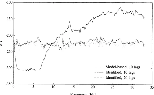
subtracting the latter from the former. The transfer functions for this Residual Generator are shown in Figure 2.5. The transfer function from y to r has a large magnitude at high frequencies. This will always be the case for practical systems as they have a natural roll-off at high frequencies. The high gain at high frequencies can be a source of trouble if we have noisy sensors or unmodelled high frequency dynamics.

The coefficients multiplying the input sequence are very small - it was first believed that this is due to the small damping in the system but it is easily shown that this is not necessarily the case. By repeating the above example and changing the damping ratio by a factor of ten to " = 0.1, we get the following coefficients:

The discretization step was also carried out symbolically and the detail can be found in

a2 al

0.01 0.002808 0.002810

0.10 0.002783 0.002797

S0 5 10 15 20 25 30 3

Frequency [Hz]

Figure 2.5: Transfer functions of the SSPR Residual Generator. The transfer functions are periodic and are shown up to half the sampling frequency.

Appendix A. We see that the elements of the A and B matrices have factors like e-

w•Ts,

cos(w, 1

0

- C2 T,) and sin(wn /1 - 2 T.). The small coefficients are a result of the product

of (, W,, and T,. Even if we had a larger damping ratio (, these elements of a will still be small because T, is small. For a given practical system we have no control over ( and the only parameter that we can vary (to a limited degree) is the sampling period.

For the single-input single-output case, the single actuator parity relation is identical to the single sensor parity relation. Therefore, only one relation exists and it is not possible to

0 -20 S-40 -60 -80 1 0n 5

Chapter 3

Displacement Sensor Failure

Detection

3.1

Introduction

In this chapter we discuss a series of failure detection experiments that were conducted on the Mini-Mast. Specifically, we will look at the detection of displacement sensor failures of the Mini-Mast and discuss several factors that influence the performance of the Residual Generators. We will also compare parity relations obtained from a state-space model with parity relations identified directly on a set of input-output data. The parity relations obtained from the state-space model will be referred to as the model-based relations and those obtained by identification as the identified relations. First, we give a brief description of the Mini-Mast.

-

Bay 18

>ensor

3

S

Z

Y

Figure 3.1: Schematic diagram of the Mini-Mast and orientation of the dis-placement sensors. The sensors measure disdis-placements normal to their surfaces, relative to a fixed structure.

Virginia. The mast is deployed vertically and is rigidly fixed at its base. It has 18 bays, each of length 1.12 meter (3.68ft); the total length of the mast is 20.16 meters (66.14ft). The bays are numbered 1 through 18, with Bay 18 at the top. The mast has three member types: longerons, battens, and diagonals. Longerons are parallel to the vertical axis and provide beam stiffness and strength in bending. Battens are in the beam face planes and provide stability. Diagonals, also in the beam face planes, provide stiffness and strength in torsion and shear. The mast is shown schematically in Figure 3.1. The truss has 57

corner joints with stainless steel pins that allow the longerons and diagonal members to be hinged, so that it is possible to retract and deploy the mast. Three torque wheel actuators

are mounted at the top of the mast parallel to the XYZ axes. By applying voltages to these motors, it is possible to apply torsional and bending torques to the mast. These actuators were used in the failure detection experiments to excite the mast. The mast is also instrumented with a full set of accelerometers, rate gyros, and displacement sensors. The displacement sensors are mounted so that each measures displacements normal to its reference surface, and relative to a fixed structure that is built around the mast. Three displacement sensors are mounted at each bay but only the three sensors at Bay 18 were used.

A finite element model for the Mini-Mast has been developed by NASA to analyze the modal frequencies and mode shapes. A brief summary is given here; detail can be found in Pappa et al. [13]. The first two modes are the first bending modes, oriented in the X and Y directions. The natural frequencies of these modes are approximately 0.65Hz. This is followed by the first torsion mode with a natural frequency of approximately 4.4Hz. The fourth and fifth modes are the second bending modes with natural frequencies of approximately 6.2Hz. The directions of the second bending modes are rotated by 45 degrees from the X-Y directions, thus coupling the bending responses. The first and second of 108 local modes, caused mainly by the diagonal members, have natural frequencies of approximately 14.8 Hz. Other modes are: second torsional at 20.86Hz, third bending modes at 29.79Hz and 30.94Hz, third torsional at 38.83Hz, fourth bending modes at 40.12Hz and 43.41Hz, fourth torsional at 54.30Hz, fifth bending modes at 66.34Hz and 70.25Hz, and fifth torsional mode at 71.88Hz. The state-space model used to generate the model-based parity relations included the first 5 modes of the system; the modal frequencies and damping ratios used are shown in Table I. The state-space model was obtained by Drs. Raymond Montgomery and David Ghosh of NASA Langley Research Center by an analysis of input-output data in preparation for the design of a control system for the Mini-Mast. The state-space matrices are given in

Table I. State-space model modal frequencies and damping ratios

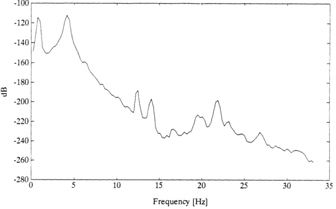
Several experiments were conducted on the Mini-Mast to obtain input-output data sets. The mast was excited by driving the torque wheels with random signals. For the experi-ments discussed in this chapter, the input signal amplitudes were independent, identically distributed with a uniform probability density function. The sampling period T, was 15 ms. This is a baseline sampling period that will be used by the control system for the mast. The input signals were held constant for four sampling periods, i.e., for 60 ms. This choice gave the freedom to simulate different sampling periods when analyzing the sensor parity relations. Unfortunately, keeping the amplitude constant for more than one sampling pe-riod but taking samples every sampling pepe-riod results in a signal with a spectrum that has zeros at frequencies lower than half the sampling frequency. A typical spectrum of an input signal that was held constant for four sampling periods but that was sampled every sampling period is shown in Figure 3.2. Fortunately, due to nonlinearities of the actuators and joints of the Mini-Mast, no zeros occurred in the output spectrum.

Mode

C

[Hz]

w

[rad/s]

First bending 0.0323 0.8559 5.3778 First bending 0.0213 0.8547 5.3702 First torsional 0.0717 4.2933 27.0133 Second bending 0.0238 6.1186 38.4440 Second bending 0.0100 6.1669 38.7478 Appendix B.

-"0 5 10 15 20 25 30 35

Frequency [Hz]

Figure 3.2: Spectrum of the input signal. The input was held constant for 4 sam-pling periods (4Ts) but samples were taken every sampling period, T, = 15 ms.

The three displacement sensors at the tip of the mast will be referred to as Sensor D1, Sen-sor D2 and SenSen-sor D3 with corresponding measurements yi, y2 and y3 and SSPR residuals

ri, r2 and r3.The transfer functions from the ith measurement yi to the ith residual ri will be called Bi(z) and the transfer functions from the inputs ul, ... , u, to ri will be denoted by Ai,1(z), ... , Ai,,(z). In some experiments we will use an increased sampling period of

30 ms, which is twice the baseline sampling period; this will be referred to as 2T,. The order of the parity relation, ni in Equation (2.25), will be referred to as the number of lags. Note that for ni lags we are actually using ni + 1 samples of the corresponding measurement:

ni past values plus the current sample. Corresponding to the 10 dimensional state of the state-space model used, the model-based parity relations incorporate 10 lags.

-30 -40 -50 -60 -70 -80 -90 -100 -110 120

-1uu -120 -140 -160 -180 -200 -220 -240 -260 -IR8 0 5 10 15 20 25 30 3-Frequency [Hz]

Figure 3.3: Spectrum of Displacement Sensor 2.

at approximately 0.9 Hz and the first torsional mode at 4.3Hz. The peaks in the spectrum

at 12.6Hz, 13.9Hz and 16.6Hz correspond to the local modes. The second torsional mode is at approximately 21.4Hz. Further, though the input signals have zeros in their spectra (see Figure 3.2), they do not show up in the spectrum of the output signal. Note that 256 point DFTs were used to compute these spectra so that we do not have very fine spectral resolution. The spectra of the other two displacement sensors are similar in nature to the

one just shown and will not be shown here. When we refer to a particular behavior of a

residual later in this work only one example will be given to illustrate the point. If a specific example does not represent all the sensors it will be noted explicitly.

The spectrum of Y2 is shown in Figure 3.3. In this figure we clearly see the first bending mode

Failures of the sensors were simulated in the data by modifying the recorded data. In most of the examples that we will discuss the sensor is failed to zero by simply zeroing the output data. (See Equation (2.7) for the modelling of failures.) We will also choose the failure times to be approximately in the middle of a plot so that it will be easy to compare the amplitude of the residual before and after the failure.

3.2

Model-based Single Sensor Parity Relations

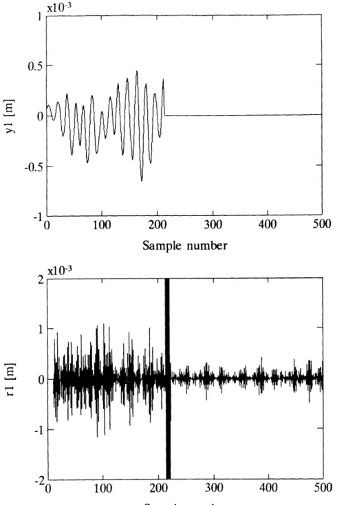
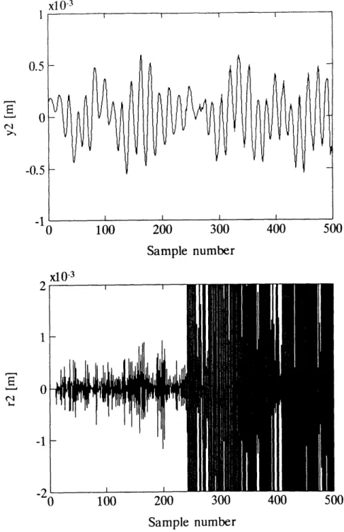
Figure 3.4 shows the failure of Sensor D1 that has failed to zero at sample number 213. The failure is clearly indicated by the large transient in the residual. In this figure we also see a behavior that was typical for all model-based residuals for displacement sensors: the residual has a large amplitude while the sensor is in perfect condition followed by a smaller amplitude when the transients excited by the failure are gone. In Chapter 2 it was shown that the inputs to the ith Residual Generator are all the control inputs and, for single sensor parity relations, the ith measurement. Equation (2.22) further shows that the ith residual ri has two components ri,, and ri,a, corresponding to the ith measurement and all the inputs. The residual is defined as the difference between these two components. Therefore, except for noise and unmodelled effects, we expect these two components to be equal. Plotting the components rl,, and ri,, separately in Figure 3.5, we see that this is not so. The component rl,, has a much larger amplitude than ri,, and there is no similarity between the two components. At first it was believed that this discrepancy is due to the small damping of the mast but the example at the end of Chapter 2 clearly indicates that this is not the reason. This difference in amplitude of the two components explains the previously mentioned behavior that the residual amplitude is large while the sensor is fully operational and small when the sensor has failed. The reason for the mismatch will be given

1

0.5

0

-0.5

1 xl 0 --0

0

100

200

300

400

500

Sample number

x10 -3 0

100

200

300

400

500

Sample number

Figure 3.4: Displacement Sensor D1 failure. Top: Sensor D1 output yl. Bot-tom: model-based

SSPR

residual rI. Sensor DI has failed to zero at sample number 213.

°. -i

2Z

I

~

0

I--1 2, 2 1

0

-1

Sx10-3

0

100

200

300

400

500

Sample number

x10

-3 0

100

200

300

400

500

Sample number

Figure 3.5: Components

ri,y

(top)

and rl,,

(bottom) of model-based SSPR

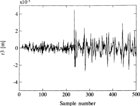
rl.

The SSPR residual r₃ is shown in the top of Figure 3.6. In this example Sensor D3 has failed to zero at sample number 235. As before, we see a large transient when the failure occurs. The bottom of Figure 3.6 shows the same residual, but this time Sensor D3 has failed at sample number 234, one sample (15 ms) earlier. Although a brief pulse is visible, we did not get a clear failure signature and the spike could have been caused by noise. This inability of the model-based single sensor parity relations to give a clear indication of sensor-off failure modes occurred often and the reason for the poor performance will be explained later. We now show a different failure mode.

A noisy sensor was simulated by adding white noise to the output of Sensor D2. The plot at the top of Figure 3.7 shows the output of Sensor D2 with noise added to it from sample number 240. The standard deviation of the noise was one hundredth that of the standard deviation of the measurement Y2. The effect of the noise is barely visible in the measurement. The corresponding SSPR residual, r2, is shown in the bottom of Figure 3.7.

The failure is clearly indicated by the residual. So the added-noise failure mode is clearly detected by the parity relation. However, this extreme sensitivity of the residual to noise can be a problem when we are working in a really noisy environment. Before we discuss the transfer functions of the Residual Generators we first turn to parity relations identified on input-output data.

2 1 -1

2-2

1

0

-1 x10-3

0

100

200

300

400

500

Sample number

x10

-3

0

100

200

300

400

500

Sample number

Figure 3.6: Top: model-based SSPR r3 when Sensor D3 has failed to zero at sample number 235. Bottom: the same residual when Sensor D3 failed at sample number 234, one sample earlier.

100

200

300

400

Sample number

100

200

300

400

Sample number

Figure 3.7: Top: Sensor D2 output. Noise was added to Sensor D2 from sample number 240. Bottom: Model-based SSPR r2.

x10

-3

1

0.5

0

-0.5

-1

x10-3

500

0

500

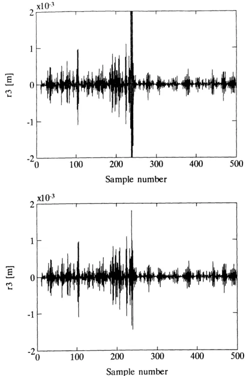
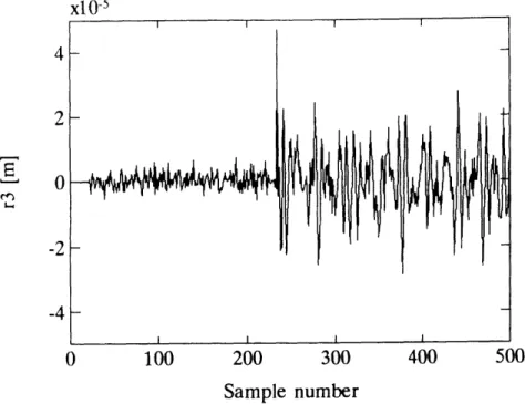
2)

-It was noted in Chapter 2 that single sensor parity relations correspond to an ARX model of the plant. Using a different set of input-output data, the coefficients of the parity relation (see Equation (2.25)) were identified using a least squares criterion. The length of the data set was slightly less than 30 seconds. These parity relations, which will be referred to as identified relations, were applied to the same data used in Section 3.2. Figure 3.8 shows

x10

5

4

2

0

-2 -4

0

100

200

300

400

Sample number

Figure 3.8: Identified SSPR residual r3. Sensor D3 has failed to z number 234. Compare with the plot at the bottom of Figure 3.6.

500

ero at sample

the identified SSPR residual r3 when Sensor D3 has failed to zero at sample number 234,

i.e., at the same time as portrayed in the bottom graph of Figure 3.6. In that case the model-based SSPR failed to give a clear indication of the failure. In Figure 3.8 we see that the identified residual gives a very different failure signature. First, note that the

amplitude of the identified residual is smaller than the amplitude of the model-based residual by approximately two orders of magnitude. Furthermore, the amplitude of the identified residual is small while the sensor is in good condition and large while the sensor is faulty, the opposite of what we had before. Clearly, this case is much closer to what we would like to see. To highlight the difference between the model-based and identified relations, we show the components r3,y and r3,u in Figure 3.9. Here we see that the contributions r3,y

and r3, are approximately of the same magnitude. We also see in these figures that the two components have similar wave forms and thus, when subtracted from each other, will result in a residual with a small amplitude. Careful comparison between Figures 3.6 and 3.9 further shows that, while the sensor is in working condition, the model-based residual has more high frequency content than the identified residual. The reason for this will become clear when we discuss the different Residual Generator transfer functions in the next section.

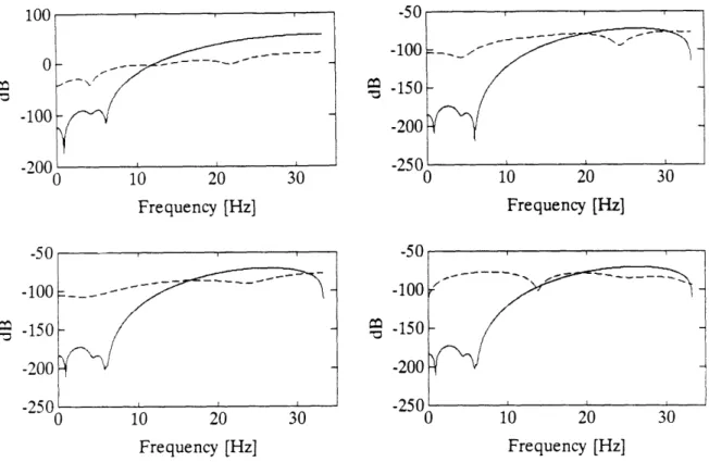
With the identified relations we have the luxury of easily increasing the number of lags used in the parity relations. In Figure 3.10 we show the residual of an identified SSPR relation with 20 lags. To make a comparison with a previous failure we have chosen a failure of Sensor D3 at sample number 234. Comparing Figure 3.10 with Figure 3.8 we see that increasing the number of lags results in a residual with a smaller amplitude while the sensor is in good health and a slightly larger residual when the failure is present. Therefore, at the expense of an increase in the number of computations, we can improve the failure signature by choosing a higher order model.

4

2

0

-2

-4

xl-

5

0

x105

500

100

200

300

400

Sample number

100

200

300

400

500

Sample number

Figure 3.9: Components r₃,y and r₃,u of identified SSPR residual r3.

xlO-

5

0

100

200

300

400

500

Sample number

Figure 3.10: Identified SSPR residual r3 with 20 lags. Sensor D3 has failed to

zero at sample number 234.

4

2

0

-2