Control of the UDS process for the production of solder balls for BGA electronics packaging

Department of Mechanical Engineering May 91997

Dr. Jung-Hoon Chun Edgerton Associate Professor of Mechanical Engineering Thesis Supervisor

Dr. Ain Sonin Chain-nan, Department Graduate Committee

B -S., in Mechanical Engineering (I 993)

Instituto Tecnologico y de Estudios Superiores de Monterrey I

Submitted to the Department of Mechanical Engineering in Partial Fulfillment of the Requirements for the Degree of

Master of Science in Mechanical Engineering

at the

Massachusetts Institute of Technology

June 1997

O 1997 Massachusetts Institute of Technology All rights reserved

Signature of Author

Certified by

Accepted by

Control of the UDS Process for the Production

of Solder Balls for BGA Electronics Packaging

by

Control of the UDS Process for the Production of Solder Balls for BGA Electronics Packaging

by

Juan Carlos Rocha Alvarez

Submitted to the Department of Mechanical Engineering on May 9 1997 in Partial Fulfillment of the Requirements for the Degree of

Master of Science in Mechanical Engineering

ABSTRACT

Size reduction of electronic components is an incessant quest in the microelectronics industry. For example, the Ball Grid Array (BGA) electronics packaging technology helps reduce the size of the electronic components while maintaining or improving their performance. The main components of the BGA technology are small solder balls, the connection elements between the chip and the circuit module or between the module and the card. The Uniform Droplet Spray (UDS) process is an efficient manufacturing process for the production of uniform solder balls that can be used for BGA packaging. This work aims at the control of the UDS process for the production of solder balls for BGA applications. The first approach used was to reduce the ball size variation by increasing the robustness of the process. At this stage the ball size variation was reduced from 9% to 2.5% of the mean ball diameter. Next a closed-loop system for mean ball size prediction and control was designed, developed and incorporated into the UDS process. The control system comprises two parts: the droplet size measurement system and the ball size control system. The droplet size measurement is based on digital

image processing, which was developed according to the Characteristics of the UDS

process. The measurement system is a precise and reliable method to determine the ball size in situ. The development of the ball size cointrol system involved the definition of a feedback signal, the development of a control algorithm, modeling, simulation, and the evaluation of the control system. The control system showed to be effective to maintain the mean ball size close to the target size. Now the UDS process is capable of accurately determining and controlling the ball size distribution. Although this work has focused on the production of large solder balls 700-800 gm), the measurement and control system can be adapted to any size of balls produced by the UDS process. However, such factors as image magnification, camera position and resolution should be considered to assure reliable, accurate ball size control.

Thesis Supervisor:

Dr. Jung-Hoon Chun

Acknowledgments

T would like to tank all the persons who made possible the completion of this work. My most sincere gratitude to:

First to my wife, Grecia, who has always encouraged me to pursuit my dreams, with unconditional love and support through all the years. My parents for all their caring and support, whose invaluable taught has leading me all my life. Prof. Jung-Hoon Chun, whose guidance and encouragement led to the success of this work. The members of the DBM group: Jeanie Cherng, Sukyoung Chey, Ho-Young Kim and Jiun-Yu Lay, without their advice, knowledge and help this work could have never been possible. Dr. Pyongwon Yim and Dr. Chen-An Chen, who helped me to start with the right foot. Dr. Nannaji Saka, for his valuable comments. Ultraclean International Co., for their help in developing the image analysis software, and for providing some equipment to accomplish

this research.

To you all,

TABLE OF CONTENTS Page Title Page I Abstract 2 Acknowledgments 3 Table of contents 4 List of Tables 6 List of Figures 7 1 INTRODUCTION 9 1.1 Introduction 9 1.2 Background 9

1.2.1 Ball Grid Array Packaging 9

1.2.2 Role of solder balls in BGA I

1.3 Mono-sized solder ball production using

the UDS apparatus 12

1.3.1 Uniform Droplet Spray (UDS) apparatus 12

1.3.2 Mono-sized solder ball production process 14 1.3.3 Characterization of solder balls produced

by the UDS process 1 5

1.4 Control approach 17

2 REDUCTION OF THE SOLDER BALL SIZE VARIATIO' 1 9

2.1 Introduction 9

2.2 Identification of sources of variation 19

2.2.1 Droplet size 9

2.2.2 UDS configuration 20

2.3 Experiments on size variation 22

2.3.1 Design of experiments 22

2.3.2 Vibration sensor 22

2.3.3 Hydrostatic pressure variation 23

2.3.4 Experimental setup 24

2.3.5 Analysis of experimental results 25

2.4 Reduction of solder ball size variation 27

2.4.1 Approach to reduce size variation 27

3 MEASUREMENT SYSTEM 30

3. i Introduction 30

3.2 Measurement system 30

3.2.1 Measurement system requirement 30

3.2.2 Digital imaging system 3

3.3 Image acquisition 3

3.3.1 Droplet trajectory 32

3.3.2 Droplet shape oscillations 34

3.3.3 Image acquisition positioning 37

3.4 Image processing 38

3.4.1 Droplet detection 38

3.4.2 Droplet measurement methods 40

3.5 Measurement method selection and results 42

3.5.1 Evaluation procedure 42

3.5.2 Evaluation results 42

3.5.3 Wavelength method sensitivity 43

3.5.4 Wavelength method resolution 44

3.6 Measurement system calibration 44

3.6.1 Camera calibration 44

3.6.2 Effect of solidification on solder ball size 45

4 CLOSED LOOP CONTROL SYSTEM 47

4.1 Introduction 47

4.2 Feedback signal incorporation 47

4.2.1 Feedback input definition 47

4.2.2 Feedback incorporation to the UDS apparatus 48

4.3 UDS process control 49

4.3.1 Time response 49

4.3.2 Steady state control limits 50

4.3.3 Control algorithm 5 1

4.3.4 Modeling and simulation of the control system 5 1

4.4 Control results 54

4.4.1 UDS system response 54

4.4.2 Sensitivity of the control system 56

4.4.3 Steady state response 58

5 SUMMARY 62

Appendix A 63

Appendix 76

LIST OF TABLES

Page

Table 1 I Influence of BGA parameters and variables 13

Table 21 Frequency effect experiments 25

Table 22 Pressure difference effect experiments 25

Table 23 Frequency effect results 26

Table 24 Pressure difference results 27

Table 31 Input parameters for the simulation 34

Table 41 Input parameter for the evaluation of the UDS process

response to the control action 55

Table 42 Input parameters for the evaluation of the sensitivity of

the UDS ball size control system 57

Table 43 Input parameters for evaluation of the steady state

response of the ball control system 59

Table 44 Properties of the size distribution for balls produced

LIST OF FIGURES

Page

Figure 1. I Pin grid array (PGA) and quad flat pack (QFP) configurations

Figure 12 BGA package

Figure 1. 3 Effect of ship interconnection technology over the package outline area

Figure 14 Droplet generator

Figure 1.5 Uniform Droplet Spray apparatus

Figure 16 SEM picture of Sn-38 wt. % Pb balls produced by the UDS process at 40x magnification Figure 1.7 Size distribution of the Sn-38 wt. % Pb balls

produced by the UDS process Figure 1.8 Solder balls possible distribution

Figure 19 Schematic of proposed closed loop control for the UDS process

Figure 2.1 Schematic of droplet formation Figure 2.2 Vibration sensor

Figure 2.3 Droplet diameter variation caused by hydrostatic pressure change

Figure 2.4 Droplet size variation from the mean due to hydrostatic pressure change

Figure 2.5 Solder ball diameter using different frequencies Figure 2.6 Solder ball diameter using different pressure

differences

Figure 2.7 Size distribution of the Sn-38 wt. % Pb balls produced by the UDS apparatus after gas control system redesign

Figure 3.1 UDS droplet size measurement system

Figure 3.2 Force balance of droplet in flight

Figure 3.3 Solder ball droplets lateral scattering

Figure 34 Solder ball droplets wavelength increment as a Rinction of flight distance

Figure -).5 Jet breakup and droplet shape oscillations at different distances from the orifice

Figure 36 Droplet roundness vs. Distance from the orifice Figure 37 Image of -750 mm Sn-32 wt. Pb droplets Figure 38 Edge detection process

Fig-Lire 39 Droplet detection process

Figle 3 1 0 Area used for the calculation of droplet size Figure 3 1 1 Measurement method variation results Figure 312 Wavelength measurement method sensitivity Figure 313 Image of solder balls used for camera calibration Figure 41 Schematic of the UDS closed loop control system

10 I 12 14 15 16 16 17 18 21 23 24 24 27 28 29 32 33 35 35 36 37 37 39 40 41 43 44 45 48

Figure 42 Flow chart of the ball size control system 52

Figure 43 UDS control system simulation results Figure 44 UDS control system feedback signal Figure 45 UDS process control response

Figure 46 Linear approximations for the measured an real ball diameter, during the control of the UDS process Figure 47 Sensitivity analysis of the controlled response of

the UDS process

Figure 48 Sensitivity analysis of the feedback control signal Figure 49 Steady state response of the controlled UDS

process for the production of solder balls for BGA

Figure 4 1 0 Feedback control signal for the control of ball size

using the UDS process

Figure 411 Size distribution for the balls produced by the

controlled UDS process

53 54 55 56 57 58 59 60 61

1.1 Introduction

New kinds of packaging technologies have been developed to accommodate the reduction in size of electronic components in the electronics industry. Among these technologies is Ball Grid Array (BGA) packaging. The BGA permits a five time size reduction compared to the most common current packaging technologies. BGA can deliver a high number of 1/0 connections while increasing the reliability of the component. The main components of BGA packaging are small solder balls: these balls are the connection element between the cp and the circuit module or between the module and the card. The current method used to produce balls for BGA is a low yield production process. Consequently the solder balls are a costly part of the BGA packaging. The Uniform Droplet Spray (UDS) process has proven to be a effective method of producing uniforin metal balls for BGA packaging technology. Nevertheless, further improvements can be made to the UDS apparatus to produce solder balls that consistently meet the high standards of the electronic industry.

This research addresses control of the UDS apparatus for the production of solder balls for BGA applications. The control of the UDS apparatus refers to the production of solder balls within a very narrow size distribution around the target size. The proposed approach to control the UDS apparatus begins with an increase in the robustness of the apparatus. At this stage, series of experiments were conducted to identify variations in the key input parameters that are associated with variations in the output (ball size variation). The apparatus was then modified to reduce such input variations; consequently, variations in the output were also reduced. Even though a considerable size variation reduction

could be achieved, it was still necessary to predict and control the mean size of the ball

size distribution. Thus, a closed loop control system was designed, developed, and implemented. This control system determines the size of the liquid metal droplet, relates

the size of the droplet to the size of the solder ball, compares the real ball size to the

target size, and then modifies the input parameters to make the ball size match the target size. This thesis describes and discusses the steps necessary to design, implement, and evaluate the ball size variation reduction and the UDS process control system.

1.2 Background

1.2.1 Ball Grid Array Packaging

An endless quest to be the fastest, smallest, lightest, and most cost effective in the electronics industry has spurred the development of new technologies. Specifically, there has been an enormous amount of development concerning chip interconnection technologies. Current interconnection technologies are concerned with providing smaller, lighter, and denser (more number of connections per unit area) electronic components. Electronics packaging reduces the size of the electronic component while maintaining or

improving its p fonnance. Specifically, chip packaging technology focuses on size reduction, higher 1/0 counts, greater density, lower cost, and higher performance. There are several methods used for electronics packaging; the most common are pin grid array (PGA) and quad flat packs (QFP). Figure 11 shows schematics of a PGA and a QFP. Ceramic PGAs were introduced in the 1960s to expand spatially dense flip chip devices. The principle of the PGA technology is to use metal pins as the connection element between the chip and the card. PGAs provide great interconnection flexibility, but offer little opportunity for pitch reduction. QFPs are characterized by the use of peripherally attached legs. The QFPs deliver a high surface mount compatibility. However, QFPs are not space efficient due to their peripheral interconnect scheme.

PGA QFP

Figure 1.1 Pin grid array (PGA) and quad flat pack (QFP) configurations.

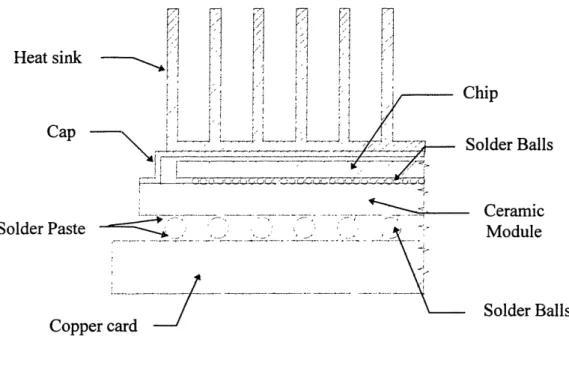
BGA is an area array interconnection technology that uses solder balls as the connection element between the chip and the module or module and card. There are three types of BGA packages, each identified by the substrate material used. These types are ceramic (CBGA), which delivers excellent thermal and electric characteristics at a relatively high cost, plastic (PBGA), which has moderate thermal and electric properties at low cost, and tape (TBGA), which has excellent thermal and electric properties at an intermediate cost. Figure 12 shows a ceramic BGA package. BGA technology provides high throughput and yields in comparison to QFP components. For example, the defect

manufacturing level for a BGA is approximately six times less thqn QFP [PuttlitZ, 1994].

Smaller and denser packages can also be produced using BGA technology. Figure 13 shows a schematic representation of the effect on chip interconnection technology on the package outline area. BGA packaging technologies have reduced the size of electronics components by more than five times. However size reduction is not the only advantage of using BGA packaging. Compared to other interconnection technologies, BGA has proven to be more cost effective and reliable. BGA packages are being considered for high 1/0 count semiconductor devices and are becoming more popular as the technology development advances, improving performance and lowering costs. he market for BGAs is expected to grow rapidly over the next few years, with BGA becoming the dominant packaging technology.

Heat sink Chip Cap Soldi Ceramic Module Solder Balls cr Balls Solder Paste Copper card

Figure 1.2 BGA package.

1.2.2 Role of Solder Balls in BGA

The performance of a BGA package depends on many parameters and variables. Table 11 [Ries et al., 1993] shows a list of parameters and variables that directly affect the BGA's reliability and yield. Solder ball size distribution directly affects the assembly reliability of the package and, indirectly, the yield. Therefore solder ball diameter must be carefully controlled to ensure assembly reliability. Ball uniformity ensures good

coplanarity of the package. Ball coplanarity for a specific ball in the array is defined by

the distance from the top of that ball to the horizontal stable sitting-plane of the package. Ball coplanarity directly determines the characteristics of the fon-nation f the final solder joints. Good solder joints reduce the probability of having bridges or opens in the connections. Most current BGA applications show a coplanarity requirement of 6 mils

[Miremadi et al., 1995] as a standard specification. Based on this specification, it has

been determined that a maximum ball size variation of ±3% from the mean ball diameter is more than adequate for BGA applications. The current research is focused on the production of large size solder balls 700 - 800 im). The UDS process to date has shown to be unable to produce large balls with such a narrow variation. One of the objectives of

the current research is to make the UDS process able to produce large solder balls with a

Area WIRE BOND - PGA Reduction Factor

0 2540 m CENTERS

WIRE BOND - SMA

2.5 1270 m CENTERS SBFC (C-4 - PGA 2.5 2540 m CENTERS SBFC (C4 - BGA !l9errvin 5.0 1270 gm CENTERS

Figure 13 Effect of chip interconnection technology over the package outline area.

1.3 Mono-sized solder ball production using the UDS process

Uniform solder balls have been produced using the UDS process [Yini et al., 1995]. The balls were made of the eutectic Sn-38wt.% Pb alloy and the process parameters were chosen to produce balls between 700 and 800 Lm. These balls showed a high level of sphericity, narrow size distribution (within ± 5% from the target diameter), uniform microstructure, and good re-melting characteristics. All the evidence collected during this study suggests that these balls can be used for BGA electronics packaging.

1.3.1 Uniform Droplet Spray (UDS) aparatus

Lord Raleigh was the first to study the dynamics of a liquid jet and its capillary instability. The UDS apparatus was developed based on the concept of Raleigh's liquid jet instability. The principal characteristic of the UDS process is its ability to produce uniform droplets. Several applications have been identified for the UDS process, including spray orming, spray coating, rapid prototyping and tooling, and uniform metal powder production.

Uniform droplet generation using the UDS apparatus is achieved through the controlled perturbation of a laininar jet of molten metal. To generate the laminar jet,

metal is melted in a crucible, then pressure is applied to force the metal out through an orifice.

ParameterNariable Influence on Package

Modules

Ball diameter Reliability

Ball cleanliness Reliability and Yield Ball attachment temperature Reliability and Yield Ball attachment time Reliability and Yield

Pad diameter Reliability

Ball planarity Yield

Ball radial error Yield

Cards

Pad diameter Reliability

Coefficient of thermal expansion Reliability

BGA site flatness Yield

Assembly process

Solder paste volume Reliability Paste deposit thickness Yield

Paste deposit error Yield

Module placement error Yield

Reflow joint temperature Reliability and Yield Reflow card temperature Reliability

Table 1.1 Influence of key BGA parameters and variables.

Vibration is imposed on the laminar jet at a desired amplitude and frequency by a piezoelectric transducer. The jet perturbation grows until the jet breaks up into uniform droplets. Figure 14 shows a schematic of the droplet generator. There are other important components of the UDS apparatus besides the droplet generator: a droplet charging system, a gas chamber, ad a monitoring system are essential for the production of uniform droplets. After the droplets are created, they experience drag forces that affect their dynamic behavior, thus different droplets have different velocities and tend to merge during flight. To avoid droplet merging, the droplets are electrostatically charged by induction charging. The process of droplet generation and charging is performed in an inert atmosphere to avoid oxidation. A monitoring system consisting of a CCD camera equipped with a macroscopic lens visualizes uniform break up of the molten metal jet into droplets. Using this monitoring system, uniform break up of the stream is guaranteed

by adjusting the parameters (vibration frequency and amplitude) until the image of the jet

breaking up into droplets freezes at the flash of a stroboscope lamp. Figure 1.5 shows a schematic of the UDS apparatus.

Thennocouple -Crucible He,, Orifice lisk transmitter I metal

0

Figure 14 Droplet generator.

1.3.2 Mono-sized solder ball production process

It was estimated that a minimum distance of six meters was required for the complete solidification of 750 pm droplets in a nitrogen environment. Since the experimental apparatus used for the present study has a maximum flight distance of one meter, a container filled with silicon oil collected and solidified the droplets. The typical procedure used to produce solder balls starts by charging the crucible with metal, then placing the top plate on the chamber and vacuuming and re-filling with nitrogen gas. After the oxygen content has been lowered to less than IO ppin, the crucible is heated to melt the metal, then a positive pressure difference between the crucible and the chamber is applied, forcing the metal out through the orifice. Then the laminar jet of molten metal is broken up into uniform droplets by adjusting the vibration frequency and amplitude. Once uniform droplets are generated, they are electrically charged to prevent merging. Immediately after the droplets are charged, they are collected into silicon oil where the balls are solidified. Finally the balls are cleaned to remove oil residue.

,' Function I Generator i --- : I Oscilloscope !, 1 Amplifier I i I - -11 Transformer i f Temperature I I, ,__ I Controller Strobe jrpv Chnmhpr Three-way valve Vent : Nitrogen _i , --- i suppl l i j. crucible -1>1 I i I 1- ! Nitrogen i i , , ! 11 supply for ; i 1 chamber F DC voltage ! : source I Video I Camera i Monitor - I Vacuum ___1 : pump

Uniform Droplet Spraj / --u"'.

1.3.3 Characterization of solder balls produced by the UDS process

Solder ball appearance, shape, size distribution, microstructure, and re-melting characteristics were analyzed. The balls showed smooth surface and good spherical shape as shown in Figure 16. Figure 17 shows the size distribution of the solder balls produced by the UDS apparatus. This graph represents the results of a typical production run to produce -780gm solder balls. The ball size variation is within 5% of the mean diameter, although IO% of the total production falls out of that range. Even though 5% is a narrow size variation for typical metal powder production, the electronics industry requires a size variation within ±3% of the mean diameter for BGA packaging. The ball produced by the UDS process showed finer grains and more uniform microstructure distribution than commercially available balls [Yim et al., 1995]. Although the solder balls produced by the UDS process showed excellent characteristics, further development of the LIDS process is needed to fully apply the process to the production of solder balls for BGA.

There are two main development areas: (1) the reduction of the ball size variation and 2) the incorporation of a system to control the mean size of the solder balls.

Figure 16 SEM picture of Sn-38 wt. %Pb balls produced by the UDS process at 40x magnification. 25% 20% 00

t

Variation from the mean

Figure 17 Size distribution of the Sn-38 wt. % Pb balls produced by the UDS process.

1.4 Control Approach

The first step towards the controlled production of solder balls was to establish a control approach. Ball oz= distributions were considered normal. Figure 1.8 shows possible ball size distributions generated by the UDS process. In this figure, the continuous line curve represents the ideal distribution where the size variation is smaller than the tolerance required by the specifications and the mean size is exactly on the target diameter. The short dashed curve shows a size distribution with a size variation so wide that many balls fall outside of specifications even though the mean size is on the target diameter. Finally, the long dashed curve represents a size distribution in which the problem is that mean size is different than the target. Here the ball size variation is small but due to the mean size position, many balls fall out of the specification limits. These distributions show two different problems: a wide size variation and placing the mean size on the target size. Previous research showed that the solder ball size variation produced by the UDS process is larger than required for BGA applications, therefore the first control step is to reduce the solder ball size variation. Solder ball size variation reduction is discussed in Chapter 2.

700 710 720 730 740 750 760 770 780 790 800 Ball Diameter

([Lm)

Figure 1.8 Solder balls possible size distribution.

Once the size variation is reduced, the mean size has to be placed on the target size. For this purpose, the proposed approach is to develop a closed loop ball size control system. Figure 19 shows a schematic representation of the proposed closed loop control system. The development of the control system is divided in two main parts: first, the incorporation of a system capable of measuring the size of the droplets in flight, discussed in Chapter 3 and second, the development of a system to control the size of the ball by modifying the inputs to the process, discussed in Chapter 4.

Target Ball Diameter

Real Ball Diameter

Schematic of proposed closed loop control for UDS process.

Chapter 2 REDUCTION OF THE SOLDER BALLS SIZE VARIATION

2.1 Introduction

This chapter describes the reduction in ball size variation. The first part analyzes the UDS process and apparatus, the second part describes the procedure sed to identify the causes of variation and the third part lists the steps taken to reduce the variation and the final results achieved. The size variation reduction is based on the hypothesis that if a reduction in the variation of the inputs of a process is achieved, a reduction in the variation of the process output will be achieved.

2.2 Identification of sources of variation

A good understanding of the modeling physics of droplet formation and the governing equations is essential to identify the most influential parameters related to droplet size. A closer look at the UDS apparatus is also necessary to detect possible areas of improvement. This section covers the governing equations that define droplet size and, based on these equations, determines the most important subsystems of the UDS process in terms of droplet size variability.

2.2.1 Droplet size

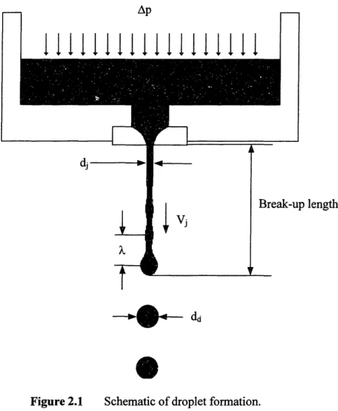
Droplet size is determined by performing a mass conservation analysis at the moment of the break up of the jet into droplets. Consider a liquid in a container that is being forced out through an orifice by a pressure difference Ap (see Figure 2 ). The jet

velocity is obtained by:

V = C. Ap (2.1)

P

where V. is the velocity of the jet, M. the discharge coefficient and, p the density of J

the liquid. Now, a pervHbation with frequency f is applied to break the liquid jet into droplets, thus the stream is broken into one droplet every I/ f seconds. It can be approximated that the jet is broken into cylinders with radius dj and length Vj / f This length is defined as the wavelength :

Vi (2.2)

Each of the cylinders transforms into a spherical droplet, thus the volume of a cylinder should be equal to the volume of a droplet, Volly = old,,,, defined by:

,-rd A Vol J (2.3) 'Y1 4 -T d Voldop = (2.4) 6

where dd is the droplet diameter. Using equations 2.3) and 2.4), the droplet diameter

can be found as:

6 A 1/3

d (2.5)

Ir

where Ai. is the cross sectional area of the jet. Assuming that the cross sectional area of the jet is equal to that of the orifice, A, and substituting equation 2.2) into equation (2.5), the droplet diameter can be calculated by:

/ 6AO Vi 1/3

dd = 7f

(2.6)

Equation 2.6) shows that droplet diameter is determined by the velocity of the jet, the vibration frequency, and the orifice area; therefore, variations in these parameters should cause variation in the size of the droplet. The velocity of the jet is controlled by the pressure difference and the properties of the liquid. Since small variations in temperature of the melt would not have a significant effect on material properties, the gas control system used to create the liquid jet is more likely to be responsible for variations in jet velocity. The breakup frequency is directly controlled by the vibration system. Although the oifice size does not have a significant effect on the size distribution, the orifice size determines the range of ball size that can be produced. The variations introduced by the gas control system and vibration control system, therefore, need to be reduced.

2.2.3 UDS configuration

The UDS apparatus is comprised of five subsystems: a vibration system, a gas control system, a melting system, a charging system, and a monitoring system. Since only the vibration system and gas control system play significant roles in droplet size determination and variability, only these systems need to be analyzed to identify possible variation sources.

An

p length

0

Figure 21 Schematic of droplet formation.

The Vibration System

The vibration system is composed of a stack of piezoelectric crystals, a holding case, a connecting shaft, and a plate. The crystals are contained in the case and transmit the vibration to the liquid through the shaft. The vibration shaft has a plate attached to its tip to assure a perturbation at the orifice. The vibration process starts with the generation of a varying voltage signal by a unction generator. The Rinction generator determines the frequency, type of the signal, and initial amplitude. Then the signal is amplified using both a variable gain aplifier and a power transformer. Finally the signal is applied to the stack of piezoelectric crystals causing a regular volume expansion and contraction of the crystals. The volume change of the crystals is proportional to the amplitude of the signal, therefore the vibration amplitude and frequency directly depend on the amplitude and frequency of the applied signal. A constant vibration frequency is essential to produce a narrow size distribution and a constant amplitude ensures a stable break up of the laminar j et.

The Gas Control System

The pressure control system consists of two compressed gas bottles, one feeding the chamber and the other feeding the crucible. The pressures at the exit of the bottles are regulated to create a constant pressure difference between the crucible and the chamber. This pressure difference forces the molten metal through the orifice, generating a laminar jet. Maintaining a constant jet velocity requires a constant pressure difference between the crucible and the chamber. During a normal operation of the UDS apparatus, low and high pressures are set at the beginning of the run.

2.3 Experiments on Size Variation

2.3.1 Design of Experiments

The procedure to determine the ball size variation was to isolate the variation produced by the two principal parameters: vibration frequency and pressure difference. Thus, two sets of experiments were designed. The first set of experiments determined the effect of frequency variation over the ball size variation. In this set of experiments, all the input parameters were held constant between experiments except the vibration frequency. The second set of experiments was conducted in the same manner as the first set, but the variable parameter was the pressure difference.

2.3.2 Vibration Sensor

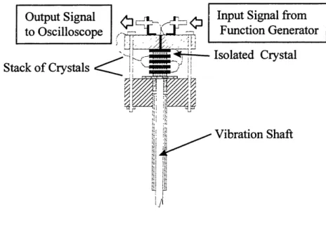
Certain problems had to be solved before performing these experiments: for instance there was not means of measuring the vibration amplitude and frequency. Therefore a vibration monitoring sensor was developed to perform these experiments. This vibration sensor was implemented by adding an extra piezoelectric crystal to the stack of crystals that generates the vibration. This extra crystal is isolated from the electric signal driving the stack. Consequently, when the stack expands, the isolated crystal contracts and generates a voltage difference. This voltage difference is monitored using an oscilloscope, on which the frequency and amplitude of the voltage coming from the isolated crystal represent the vibration frequency and amplitude of the atual perturbation. Figure 22 shows the vibration sensor. This vibration sensor ensures that the same vibration amplitude is used during and between each experiment. The sensor also allowed the determination of the best parameters to obtain a clean output from the vibration system. A clean output is defined by the similarity between the signal that comes from the vibration sensor and the electric input in terms of frequency and shape. In other words, if a 1000 Hz sinusoidal signal is applied to the apparatus, the output from

After running the UDS apparatus using square, triangular and sinusoidal signals, it was deten-nined that the cleanest vibration output at low frequencies 800-2,000 Hertz) was produced by using a sinusoidal input signal, thus this signal is used to perfon-n all experiments.

I - - I T--- nl---- L---- I

Uutput signai

to Oscilloscol Stack of Crystals

Input Signal from Function Generator Isolated Crystal

Vibration Shaft

Figure 22 Vibration Sensor.

2.3.3 Hydrostatic pressure variation

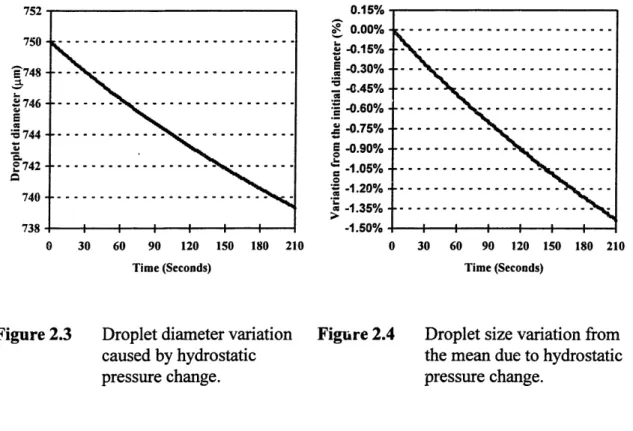
An important source of droplet size variation is the change of hydrostatic pressure during a run of the UDS apparatus. his hydrostatic pressure is produced by the weight of the molten metal contained in the crucible and depends on the height of the column of metal above the oritLice. Thus, as the metal is ejected from the crucible, the hydrostatic pressure decreases along with the column of metal. As the .- Mure ecreases, the jet velocity Vj decreases causing a decrease in the droplet diameter. Figure 23 shows the predicted decrease in droplet diameter as a fnction of ran time. This calculation was made considering the current crucible geometry, using 0.5 kg of Sn-38 wt.% Pb a 406gm orifice, and a pressure difference of 34.4 KPa. Figure 24 shows the percentage size variation from the initial droplet diameter of 750gm. The magnitude of the variation produced by the change in hydrostatic pressure depends on the configuration of the crucible and the target droplet size. Nevertheless, the variation produced by hydrostatic pressure can be significantly decreased by using a short collection time. For example, for a batch of 750gm solder balls collected during a 30 second period, only 0.14% of the total size variation would have been caused by changes in hydrostatic pressure.

0.15%

0.00%

--

---0.15%

-

-1.05%

---

...

For the current study, all the experiments were evaluated using a collection time of 30 seconds. By doing so, the effects of ball size variation caused by hydrostatic pressure were minimized, and the observed variation was only due to variations in the pressure difference or vibration frequency. Since the change in hydrostatic pressure has gradual (long time constant) effects over ball size variation; this variation can be easily controlled by a feedback control system. Therefore, no attempts were made to reduce the change in hydrostatic pressure by modifying the UDS apparatus.

752 750 'j74 4'746 -Z S M :6 744 -Z 10 742 -12 740 I

---...

---

...

...

Figure 23

caused by hydrostatic pressure change.

Droplet size variation from the mean due to hydrostatic pressure change.

2.3.4 Experimental Setup

Frequency effect experiments

A set of experiments was performed to determine how frequency variations affect the ball diameter distribution (mean and variance). These experiments were performed by setting up the constant input parameters at the beginning of each run. The parameters were held constant at a point where the UDS apparatus output was most stable. Table 21

shows the values of the constant parameters. The vibration frequency was closely monitored during the run to avoid variations. The experiments were perfonn,-d at frequencies of II 80, 1362, 1447 and 1568 Hertz.

Pressure Difference 34.4 K-Pa Vibration Amplitude 0.9 V

Charge Voltage 3 KV

Orifice Diameter 406 tm

- Si2al Shape Sinusoidal

Vibration Frequency 1492 Hertz Vibration Amplitude 0.9

Charge Voltage - 3 KV

Orifice Diameter 406 Lm

Signal ShMe Sinusoidal

Table 21 Frequency effect experiment parameters.

Pressure difference effect experiments

A set of experiments was performed to determine how pressure difference variations affect the ball diameter distribution. These experiments were conducted in the same manner as the frequency effect experiments. The input parameters were fixed at the values shown in Table 22. Balls were produced, collected, and measured using pressure

differences of 20.3, 29.6, 36.8, and 45.1 KPa.

Table 22 Pressure difference effect experiment parameters.

2.3.5 Analysis of experimental results

Frequency effect results

Table 23 and Figure 25 show the results of the frequency effect experiments. In Figure 25, the mean of each experiment is represented as a single point, the error bars at each point represent the range in which 95% of the total production is located (size variation), and the continuous line represents the ball diameter calculated from equation 2.6 using the parameters shown on Table 21. The percentage of the production that is within ±Y/'U of the mean diameter is used as the erformance evaluation parameter. Table 2.3 shows that in three out of four experiments 85% of the total production is within ±3 %. The best run was at 1447 Hz, and the worst at II 0 Hz.

Exp. Frequency Mean Std. Deviation Production

# - (HeEzj icromete (Micrometers) within ±3%

1 1180 820.42 42.99 43.3

2 1362 787.89 16.89 83.81

3 1447 742.77 14.49 87.58

4 1 1568 744.00 1 15.35 1 85.41

These results show that uniform break up can only be achieved within a defined range of frequencies for a given jet diameter. As the frequency goes closer to the borders of this range, the break up becomes unstable, generating non-uniform droplets with a very large size variation. Thus, it is highly probable that II 0 Hz is close to the unstable break up border, explaining why only 43.3 of the production was within ±3% of variation.

Referring to Figure 25, the experimental results show a decreasing trend in ball diameter as the driving frequency is increased, but note that the mean ball diameter of the experimental results is consistently smaller than the theoretical predicted value. This can only be explained by a systematic variation in the pressure difference, since the pressure difference is the only "constant" input that can significantly affect the ball diameter.

Table 23 Frequency effect results.

Pressure effect results

Table 24 and Figure 26 show the results of the pressure difference effect experiments. In Figure 26, the mean of each experiment is represented as a single point, the error bars at each point represent the range where 95% of the total production is located (size variation during an experiment), and the continuous line represents the ball diameter calculated from equation 2.6) using the parameters shown in Table 22.

Figure 26 shows that the pressure effect experiments had better results than those obtained by the frequency effect experiments. The mean ball diameter of three out of four experiments coincides with the theoretical value. Therefore, it can be concluded that there was no significant variation in te constant parameters. Te difference in results from the frequency effect and pressure, difference effect experiments confirms that the pressure difference is the source that produces size variation, because during the pressure effect experiments a constant pressure difference was maintained throughout the collection time. Table 24 shows that the percentage of the production within ±3% increased considerably. Among these experiments, the best run used 29.6 KPa of pressure difference: in this run almost I 0% of the balls were within ±3 %. Hence, for a 406 gm jet diameter breaking up at a frequency of 1492 Hz, the optimal velocity is generated with 29.6 KPa of pressure difference.

A Dd f- I 80 X DdfL1362

I 6 Dd P-1447 N Ddf--1568

I -Dd Calculated using eq. 2.6)

Exp. Pressure Mean Std. Deviation Production

Difference (Micrometers) (Micrometers) within %

(KPa 1 20.3 701.21 11.01 94.38 % 2 29.6 739.45 7.99 99.44 % 3 36.8 786.89 21.87 71.98 % 4 1 45.1 753.70. 1 12.70 88.24 % 950 , i I - 900 E =L I I 850 T_I Q 4-15 E 800 4-cc 9Z 750 1_I 1200 1300 1400 Freqaency (Hz) 1500 1600 1100

Figure 25

These experimental results show that having better control over the pressure difference will allow production of balls with a size variation within ±3% of the mean diameter. Therefore, the gas control system has to be redesigned to reduce its variation.

Table 2.4 Pressure difference effect results.

2.4 Reduction of solder ball size variation 2.4.1 Approach to reduce size variation

Once the cause of solder ball size variation was identified, the next step was to redesign the gas control system to reduce pressure difference variations. The main objective of the gas control system is to maintain a constant pressure difference between the crucible and the chamber. The previous experiments showed that the pressure control was deficient, requiring a change in the system.

900 1-1 I E 850 11 =L 1-1 L. 800 0 .0. 'V 750 9 I es 700 rZ I '<9n -i 13 19 25 31 37 43 49

Pressure difference (KPa)

EDd 20.3 A Dd 29.6 X Dd 36.8 0 Dd 45.1

Dd Calculated using eq. 2.6)

Figure 26 Solder ball diameter using different pressure differences.

The pressure was controlled by two single stage pressure regulators. These type of regulators have two main disadvantages. The first one is lack of accuracy, this means that they have to be calibrated before using them. The other disadvantage is that these regulators are one-way regulators. For example, if pressure builds up in the chamber during a run, the low-pressure regulator is not able to exhaust the excess of pressure, resulting in a decrease of the pressure difference between the chamber and the crucible. In fact, pressure builds up in the chamber during a normal solder ball production run. The pressure difference can vary up to 13.7 KPa during a three minute interval. Assuming that if constant pressure difference can be maintained throughout the production time, the only source of variation should be changes in hydrostatic pressure, two new pressure regulators were incorporated to the gas control system. One of them controlled the pressure applied to the crucible, and the other controlled the chamber pressure. These are high precision pressure regulators (Omega PRG101-60). These pressure regulators have a precision measurement capsule and a high gain servo aplifier. Whenever the pressure builds up, the regulator exhausts the system with a response time of 02 seconds to a 0% flow change. The most iportant feature of these regulators is that they can maintain a constant pressure within ± 35 Pa of the setpoint.

2.4.2 Size variation distribution results

Figure 27 shows the ball size distribution after the new pressure regulators were incorporated into the UDS apparatus. These results show that 100% of the production is within ±2.5% of the mean diameter. Comparing Fig. 27 to Fig. 17 a drastic reduction in ball size variation can be clearly observed. By the use of these regulators, variations due to pressure settings and increase in chamber pressure were minimized. The UDS process is now perfectly able to produce solder balls for BGA electronics packaging within the specified size variation.

The next step following the proposed control approach is to locate the mean ball size on the target size by implementing a feedback control. The next two chapters cover the development and implementation of the feedback control system.

25% . . . . 20% r Z .00 0 I-0. 9 0 15% 10% - - - --- - - -I .... :. . . . i 1.0% 1.5% 20% 25% 30% 5% 0%, -3.0% 25% 20% -1.5% -1.0% -0.5% 0.5%

Variation from the mean

Figure 27 Size distribution of the Sn-38 wt. Pb balls produced by the UDS

Chapter 3

3.1 Introduction

The first step in the implementation of a closed loop control system was the

development of a system to measure droplet size in flight. The most significant decision guidelines in choosing the measurement system were accuracy and speed. The proposed system had to be accurate within micrometer precision to detect small droplet size variations. It also had to be fast enough to detect any small variation before the variation grew out of the control limits. Considering these two guidelines, it was decided to use image analysis to determine the droplet size. Image analysis has the potential to deliver both speed and accuracy at the required levels. The development of the system started by determining the best place to take the image along the stream of droplets; this decision was based on droplet trajectory and shape oscillations. Then a image processing system was developed according to the special characteristics of the process. Several

measurement methods were implemented and evaluated. The result was the incorporation

to the UDS process of an effective and reliable system to determine the droplet diameter during production. This chapter deals with the customization and measurement methods needed to deliver precise, accurate, sensible and high resolution measurements of the droplet size.

3.2 Measurement system

3.2.1 Measurement system requirement

The UDS process and apparatus determined the type of imaging system chosen. For example, an important apparatus constraint is that the measurement has to be performed outside the pressurized chamber; thus, the measurement system has to be able to perform the measurements from a distance at least 8.5 cm from the stream of droplets. The system also has to measure droplets traveling at speeds up to 12 m/s and make these measurements fast enough to detect any variation quickly. The resolution of the measurements has to be much less than the size variation in the droplets caused by

variations in process conditions. In this way, any small variation in droplet size can be

detected. Another important aspect to be considered in deciding the type of the measurement system is integration into the closed loop control system. Digital imaging was chosen as the measurement method mainly because of its high capability of integration and customization. Digital imaging can satisfy all the constraints previously mentioned, but its key advantage over other measurement is the ease of integration and custornization.

3.2.2 Digital Imaging System

A continuous representation of an image cannot be conveniently interpreted by a computer, therefore, an alternative representation, the digital image, must be used. This digital image is generated by an analog-to-digital converter, often referred as the "frame grabber." Using a frame grabber, the digital image can be stored into the frame memory, allowing data processing and display. The proctss of grabbing i image is as follows: the image is picked up by an electronic device (usually a CCD camera) the video signal then is conditioned, synchronized, and digitized. For the digitizing step the frame grabber uses a converter that samples the analog signal to discrete time intervals and converts each sample to a digital element called a pixel. These samples (pixels) have certain intensity

levels that usually range from to 255, i.e. 256 levels of gray. The digitized image is

represented by a two dimensional array of pixels, each pixel having a value between and 255. This array size depends on the resolution of the camera and frame grabber.

A digitized image can be easily processed by a computer, as long as there is an

interface between the frame grabber and the computer. For the current research, a PCI local bus frame grabber (Data Translation, model DT3155) was used. This frame grabber

has a 8-bit converter and 256 levels of gray. The image is acquired by a high resolution

CCD camera (Pulnix Co., TM-7X). This camera has a 768 (horizontal) x 494 (vertical) pixel array and a shutter speed of 130 sec. For the resolution required for a satisfactory measurement of the droplet size, a zoom macroscope tube (Meijilabax, UNIMAC) and an

auxiliary lens of 0.5X are attached to the camera. This tube and lens provides a

magnification of 35 - 22.5X at a working distance of approximately 15 cm. Ile frame grabber is placed on a PCI 32-bit bus master expansion slot of a personal computer (DELL, Dimension Pro2OOn), on which a customized image processing software was

developed to measure the droplet size. The software development is covered on the next

section of this chapter. Another important part of the imaging system is a stroboscope

lamp (Pioneer, DS-303). This lamp flashes at I I 0 the frequency at which the droplets are being generated. In this way the image of the droplets is frozen and the camera can

acquire a clear image. Figure 31 shows a schematic representation of the digital imaging measurement system.

3.3 Image acquisition

The camera position along the stream of liquid droplets is crucial for the development of a reliable measurement system. This positioning depends on factors such as droplet trajectory and droplet shape oscillations. This section covers the basic principles of these factors, and explains the decision process followed to determine the

i i

I F Auxiliary lens

)boscope I

Lamp Zoom macroscopic tube

CCD Camera Analogue Imqge , I f I I : 1 1 -- I - , , Analogue X z !iglw . ... ... ... I... : V I J y Frame grahher I - cl-

--Computer motherb Digitized ::

image ...

COMPUTER

Figure 31 UDS droplet size measurement system.

3.3.1 Droplet trajectory

A good understanding of droplet trajectory is essential to ensure that the acquired image represents the actual droplet size. The positions of the droplets change as they travel down due to the drag, electric charge, and gravitational force. As the droplets travel, they experience drag force which attenuates the droplet velocity. The drag force

can be found as:

2 I.V .V

Fd= Cd (Pi _-P9 Md _{4 2}--

(3.1)

where Cd is the drag coefficient, pthe liquid density, pg the gas density, dd the

dropletdiameterand V istherelativevelocityofthedropletwithrespecttothegas.

Another important force acting on the droplets is the one caused by the droplets' electric charge. As explained before, the UDS apparatus induces an electric charge to the droplets to prevent merging.

This electric charge produces an electro-repulsion force, called the Coulomb force: 2

F

e 4)r6o r2 (3.2)

where co is the permittivity of free space, r the distance between the two interacting droplets, and qd is the amount of charge induced in each droplet. The charge can be

obtained from (Passow, 1992):

qd = - 2 ire 0 vj V

In(d, / dj) f

where v is the jet velocity, dj the diameter of the jet, d, the diameter of the charging ring, f the driving frequency, and V the charging voltage. The last force affecting the

droplets is the gravitational force, expressed as:

IrdP

P9 = 6 d k (3.4)

Figure 32 shows a schematic representation of a droplet in flight. From this figure and using the previous equations, the equation of motion for a droplet becomes:

n

Md =

_{d, + P, + E Pe,}

(3.5)

where di is the acceleration of the droplet i , number of droplets surrounding the droplet i .

m the mass of the droplet and n the total

Fd ir+2 I -i i FeiI /M -- i+n Fei2 of droplet in flight. I/ i n Fe, i+1

Figure 32

Material Sn-32wt.% Pb Pressure Difference 34.4 KPa

Frequency 150 Hz

Vibration Aplitude 0.9

Signal Shape _ Sinusoidal

Charge Vo tage I KV

Orifice Diameter 4 0 6 -l

Various numerical simulation codes have been developed to determine the scattering of the droplets produced by the UDS apparatus. Figures 33 and 34 show the results of a numerical simulation (Abel, 1993). The parameters shown in Table 31 were used to run the simulation of the production of -750gm Sn-38 wt.% Pb. Figure 33 shows the lateral scattering. The droplets start to deviate from the center at cm from the orifice, growing exponentially as the distance increases. The lateral deviation is insignificant at distances smaller than 15 cm, so that if a image is taken within 1 cm fTom the orifice, lateral scattering will not affect the precision and accuracy of the image. However, there is still scattering in the y-direction. As the droplets travel down the wavelength A increases. This wavelength increase is caused by the electric repulsion force experienced between neighboring droplets. Figure 34 shows the increase of the

wavelength A as a function of the distance from the orifice. The continuous line shows

the numerical simulation results while the cross noints show the wavelength variation determined by measuring the distance between droplets directly from the images shown

in Figure 35. The wavelength can be used to determine droplet size as shown in Equation

2.5. However, the value of the wavelength just after breakup should be used. Therefore, any image that involves the wavelength to determine droplet diameter should be acquired before the wavelength increase becomes significant. For the production of -750gm solder balls, the wavelength increase becomes significant at cm from the orifice, thus, the image should be acquired within this distance. There is yet another factor to consider in positioning for image acquisition. This factor is droplet shape oscillations and will be covered in the next section.

Table 31 Input parameters for the simulation.

3.3.2 Droplet shape oscillations

The process of droplet formation can be divided in six stages (Peregrine et al., 1989). The first is necking of the liquid stream: Figure 35 a) shows how the perturbation in the stream surface grows until it generates a very thin cylindrical column bridge that connects the stream to the nascent droplet. The second stage consists of the bifurcation of the main drop; it is at this stage that the droplet separates from the stream (Figure 35 b). Recoil is the stage which occurs immediately after droplet separation. Recoil is caused by the unbalanced surface tension that rapidly accelerates liquid in both bodies, droplet and stream.

15 450

'i

E 400

---

---250

---

0 6 10 is Distance from the orifice

Distance from the orifice y-direction (cm) y-direction (cm)

x-direction - z-direction Simulation X Experimetnal Figure 33 Solder ball droplets lateral Figure 34 Solder ball droplets

scattering. wavelength increment as

a function of flight distance.

The newly generated droplets show a strong defon-nation at this stage. Figure 35 c) shows an apparent flattening of the top of the newly generated droplet. This is in fact

the rim of a depression in its surface. The fourth stage is wave generation, which takes

place when the recoil effects propagate onto the cylindrical remain of the liquid bridge. This stage is characterized by the formation of growing waves in the cylindrical bridge caused by the conversion of the potential energy of the surface of the cylinder into wave motion. Figure 35 c) shows the wave generation at the bridge. The fifth stage consists of a secondary necking and biffircation, occurring on the cylindrical bridge and resulting in the formation of a secondary droplet. Figures 35 b) and c) show this stage. The sixth and final stage consist in the coalescence of the main drop and the secondary drop (Figure 35 c)). After the main and secondary droplets merge, the droplet still shows the effects of the recoil stage with shape oscillations. These shape oscillations decrease in amplitude until the surface tension balances and the droplet is completely spherical. Figures 35 d) through j) show the droplet shape oscillation behavior during a typical run for the production of solder balls. The sphericity of the droplets as a function of the distance from the orifice was determined based on the images of Figure 35. Figure 36 shows the sphericity of the droplets at different distances from the orifice, where the sphericity was estimated by comparing the maximum horizontal and vertical droplet diameters. The sphericity of a droplet is defined as:

max(DOhorzontal 100%)

(3.6)

max(Dd )verfi.1

where represents the sphericity of the droplet, where = I 0% represents a perfectly spherical droplet.

C) a) d)

w

0

Jet break-up and droplet shape oscillations at different distances from the orifice. This images correspond to a typical ran to produce 750 gm balls of Sn-38 wt. Pb.

Figure 35

f t I

3.3.3 Image acquisition positioning

Analysis of droplet trajectory and shape oscillations suggests that the camera can be placed within 15 cm from the orifice if the image processing does not use the wavelength to calculate the droplet diameter, and within cm if the wavelength is used. Droplet shape oscillations, however, present difficulties in determining the droplet diameter by direct measurement of the droplet. Based on the results shown in Figure 36, it takes about 20 cm for the droplets to become spherical. Unfortunately when the droplets are completely spherical, they already have started to scatter, and are outside the depth of focus of the camera.

100%

...

...

...

y-direction (cm)

Figure 36

Considering droplet trajectory and shape oscillations conditions during ball production, the best place to position the camera is within cm from the orifice. Figure 3.7 shows a typical image used to measure droplet size. At this position the droplets are not completely round ( = 8 - 5% ), thus the accuracy of the measurement strongly depends on the measurement method used.

''Ofifi-e , ` 11'-"-"

Figure 37 Image of - 750 pm Pb-38 wt. % Pb droplets. The image size is 480(V) x 640(H) pixels.

3.4 Image Processing

Once the image acquisition system was incorporated into the UDS apparatus and the determination of the image acquisition position completed, the next step was to determine the kind of image processing that should be done to obtain precise measurements of the droplet size. Image processing is divided in two stages: droplet detection and droplet measurement method. Each one of these stages contributes to the precision and accuracy of the measurement, therefore a careful definition and evaluation was performed at every stage.

3.4.1 Droplet detection

The first step in droplet detection is to identify the droplets in the image; the detection process is based on edge detection. Edge detection consists of the detection of discontinuities, places with an abrupt change in gray level, indicating the end of one

region and the beginning of another. Figure 38 shows the edge detection process in a

image of a droplet. The image of the droplet edge results in an intensity distribution consisting of a step-like function (Figure 38 a). It is commonly assumed that the actual position of the edge is either where the gradient has its maximum absolute value (Figure

3.8 b), or where the second derivative (Laplacian) has zero value (Figure 38 c). The

following equation calculates the gradient of a digitized image from the definition of a derivative of a ftinction:

f W = lim f (X + Ax) f W

(3.7)

AX-+0 AX

the closest an image of distinct pixel values can get to Ax > 0 is unity, thus for digital

images, differences are used instead of derivatives. The best approximation of the partial derivatives in the x and y directions are:

S = fX + 1 Y) f(X' Y) (3.8)

S = X + ) - f (XY) (3.9)

where f (xy) is the level of gray of the pixel located at (xy) coordinates. This simple approximation is very susceptible to noise, because of the way it estimates is directional derivatives. Thus, an alternative method was used to find the droplet edges. That method involves the combination of the difference process and moving averages. This edge detection method uses 2n number of pixels to calculate the difference of the pixel

-I 0 10 iO 30 40 60 60 : Pixels - . '. - . / I ; W 30 40 60 60 : Pixels : n n

Ef (xy+n) -Yf (xy -n)

I I n .1 - z I I I I I -;, 300 co 1. U 200 1-0 a) W 100 It U b) r-C) L JVO V 30 40 Pixels I .L

Edge detection process.

The following equations show the difference equations used to find the edge:

n n

Zf(x+ny)-Zf(x-ny)

=

In the current edge detection algorithm, n was chosen to be 16 of the estimated droplet diameter measured in pixels.

The droplet detection process starts to scan every 16 Dd Clumns by looking for maximum and minimum edges within the same row. This scanning process begins from the center of the image towards the sides. When the process finds a maximum and a minimum edge in the same row, it compares the distance between these two edges to the estimated droplet diameter. Once this comparison is satisfied, the process assumes that there is a droplet between that maximum and minimum edges. After the droplet is identified, the process starts to scan the area in which the doplet was found, first row by row looking for maximum and minimum edges within the same row; and then column by column looking for maximum and minimum edges within the same column. Figure 39 shows a schematic representation of the detection process. At the end of the scanning process, the exact position of all the horizontal edges, vertical edges, and centers is known. The droplet detection algorithm was developed using Microsoft Visual C+. The source code for droplet detection can be found in Appendix A under the name of Process.c++.

-No-

-0-

-0-Droplet localization Horizontal edge Vertical edge Horizontal

detection detection vertical edges

and centers Figure 39 Droplet detection process.

3.4.2 Droplet measurement methods

Two types of measurements can be made using the data generated by the droplet detection process. Te first type is direct measurements: the droplet size is directly determined from the size shown in the image. The second type of measurements is indirect measurements: here the measurement is made over a parameter that correlates either physically or geometrically to the droplet size. The droplets contained in a typical image are not spherical because of droplet shape oscillations. Therefore, using a direct measurement method reduces the precision and accuracy of the measurement while indirect measurement avoid this pitfall. Four different methods were studied. The first one is a direct method that uses horizontal and vertical diameters to determine fal droplet diameter. The following equations show the relation between measurement and real droplet diameters:

Dd MaX(Dd)h,,,i..Il

(3.12)

or:

where Dd is the real droplet diameter, max(Dd)h,,,i,,,,,,,,,/ the maximum horizontal droplet width, and max(Dd),,,,jj,,,,j the maximum vertical droplet width. The second method determines droplet diameter by using the total area of the droplet. The area of a droplet is determined by counting the number of pixels that are enclosed in the perimeter of the droplet. This perimeter is defined by the position of all maximum and minimum edges, as shown in Fig. 3 1 0. The droplet diameter is then calculated by assuming that the total area of the droplet at the time of the image represents the total cross sectional area of the

droplet. The droplet diameter can be found as:

7CI

(Dh.,)

D 1 (3.14)

d 4

where n represents the total number of rows included in the droplet and Dhn the droplet

horizontal width at the n row.

El

Figure 310 Area used for the calculation of the droplet size.

The third measurement method involves the calculation of the volume of the droplet in the image. For this method to work, y-axis symmetry has to be assumed. The volume of the droplet can be determined by slicing the droplet in plates one pixel thick on the horizontal direction. Based on the y-axis symmetry assumption, these plates are considered circular with the center located on the y-axis. The diameter of these plates is equal to the droplet vertical width at that point along the y-axis. The total volume of the droplet is then calculated by adding the volume of all plates. The following equation shows the method of calculation:

3 1/3

.-ij(D'

(3.15)

Dd = 2 ver

where i is the total number of columns contained in the droplet and Dv,,, the droplet vertical width at the i column. The last measurement method involves a physical relation