Convergence speed in distributed consensus and averaging

Convergence Speed in Distributed Consensus and

Averaging

by

Alexander Olshevsky

Submitted to the Department of Electrical Engineering and Computer

Science

in partial fulfillment of the requirements for the degree of

Master of Science in Computer Science and Engineering

at the

MASSACHUSETTS INSTITUTE OF TECHNOLOGY

@

Massachusetts

May 2006

Institute of Technology 2006. All rights reserved.

Author ....-.... o... .-. ,,...,'ý ...

Department of Electrical Engineering and Computer Science

May 25, 2006

Certified by ...

.p

John N. Tsitsiklis

Professor

Thesis Supervisor

Accepted by.

Arthur C. Smith

Chairman, Department Committee on Graduate Students

LIBRARIES

ARCHIVES

NOV 0 2 2006

. ...

.

.

. . . .

Q: - ý'.

_...

_...

E

Convergence Speed in Distributed Consensus and Averaging

by

Alexander Olshevsky

B.S. Applied Mathematics (2004)

B.S. Electrical Engineering (2004)

Georgia Institute of Technology

Submitted to the Department of Electrical Engineering and Computer Science on May 25, 2006, in partial fulfillment of the

requirements for the degree of

Master of Science in Computer Science and Engineering

Abstract

We propose three new algorithms for the distributed averaging and consensus prob-lems: two for the fixed-graph case, and one for the dynamic-topology case. The convergence times of our fixed-graph algorithms compare favorably with other known methods, while our algorithm for the dynamic-topology case is the first to be accom-panied by a polynomial-time bound on the worst-case convergence time.

Thesis Supervisor: John N. Tsitsiklis Title: Professor

Acknowledgments

I am grateful to my advisor, John Tsitsiklis, for his invaluable guidance and tireless efforts in supervising this thesis. I have greatly benefitted from his help, suggestions, insight, and patience.

I want to thank Prof. Vincent Blondel and Prof. Ali Jadbabaie for useful conversa-tions that have helped me in the course of my research.

I want to thank Mukul Agarwal, Constantine Caramanis, and Aman Chawla. I have learned much from my conversations with them.

I thank my parents for all the encouragement they have given me over the years. Finally, I want to thank Angela for her constant support.

This research was supported by the National Science Foundation under a Graduate Research Fellowship and grant ECS-0312921.

Contents

Products of stochastic matrices and convergence rate . . . . Convergence in the presence of delays . . . . . . . . . ..

3 Nonexistence of Quadratic Lyapunov Functions

4 Averaging with the agreement algorithm in fixed networks

4.1 Using two parallel passes of the agreement algorithm ... 4.2 Comparison with other results . ...

5 Estimates of the Convergence Time

5.1 Convergence time for the equal neighbor time invariant model 5.2 Symmetric eigenvalue minimization via convex optimization

5.2.1 Problem description . . ... 5.2.2 Relaxing the constraints . . ...

5.2.3 Our contribution . . . ...

5.2.4 Convergence rate on a class of spanning trees . . . . .

5.2.5 Bounding the second eigenvalue . ...

5.2.6 Eigenvaliue optimization on the line . ...

41 . . . . 42 . . . . 44 . . . . 44 . . . . 45 . . . . 45 . . . . 46 . . . . 47 . . . . 48 2 The 2.1 2.2 2.3 11 11 13 17 17 19 22

5.3 Convergence time for spanning trees ...

6 Averaging with Dynamic Topologies 55

6.1 Exponential Convergence Time for the Agreement Algorithm . . . . 55

6.1.1 Construction . ... ... . ... . . 56

6.1.2 Analysis ... ... ... ... .. 58

6.2 Description of the Algorithm ... ... 59

6.3 Convergence Time ... ... ... . 60

7 Simulations 65 7.1 Averaging in fixed networks with two passes of the agreement algorithm 65 7.2 Averaging in time-varying Erdos-Renyi random graphs ... . 68

List of Figures

3-1 The nodes perform an iteration of the nearest-neighbor model with this graph. Every node has a self-loop which is not shown in this picture. 30

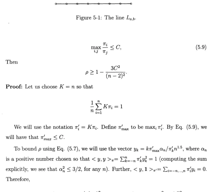
5-1 The line La,b. ... . ... 49

6-1 The iteration graph at time 0. Self-loops which are omitted in the figure are present at every node. . ... .. 56

6-2 Iteration graph at times 1, ... , B - 2. Self-loops which are omitted in

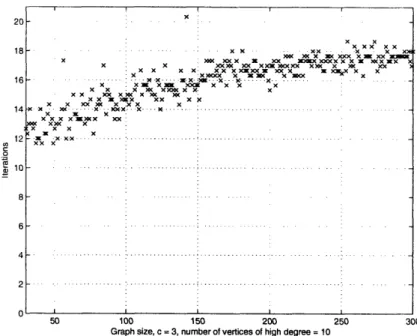
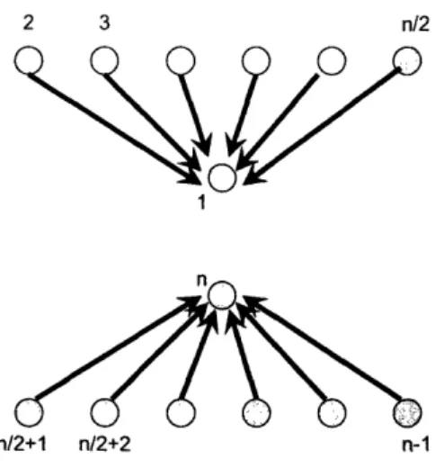
the figure are present at every node. . ... 57 7-1 Comparing averaging algorithms when c = 3. The top line corresponds

to the algorithm of [32], and the bottom line corresponds to two parallel

passes of the agreement algorithm. . ... 66

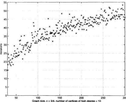
7-2 A blow up of the performance of the agreement algorithm when c = 3. 67 7-3 Comparing averaging algorithms when c = 3/4.The top line

corre-sponds to the algorithm of [32], and the bottom line correcorre-sponds to two parallel passes of the agreement algorithm. . ... . . 67 7-4 A blow up of the performance of the agreement algorithm when c = 3/4. 68 7-5 Averaging in time-varying Erdos-Renyi random graphs with the load

balancing algorithm. Here c = 3 at each time t. . ... 69

7-6 Averaging in time-varying Erdos-Renyi random graphs with the load

Chapter 1

Introduct ion

1.1

Motivation

Given a set of autonomous agents -- which may be sensors, nodes of a communication network, cars, or unmanned aerial vehicles - the distributed consensus problem asks for a distributed algorithm that the agents can use to agree on an opinion (represented by a scalar or a vector) starting from different initial opinions among the agents and possibly severe restrictions on communication.

Algorithms that solve the distributed consensus problem provide the means by which the networks of agents may be coordinated. Although each agent acts inde-pendently of the others, because the agents can agree on a parameter of interest, they may act in a coordinated fashion when decisions involving this parameter arise. Synchronized behavior of this sort has often been observed in biological systems [19]. The distributed consensus problem has historically appeared in many diverse ar-eas: communication networks [29, 26]. control theory [23], and parallel computation [38. 5]. Recently, the problem has attracted significant attention [23, 26, 3, 14, 29,

10. . 30. 31]; research has been driven by advances in communication theory and by new connections to open problems in netwvorking and networked control theory. We briefly describe some more recent applications.

nodes of a wireless multi-hop network are not controlled by a single authority or do not have a common objective. Selfish behavior among nodes (e.g., refusing to forward traffic meant for others) is possible, and some mechanism is needed to enforce coop-eration. One way to detect selfish behavior is reputation management: each node forms an opinion by observing the behavior of its neighbors. One is then faced with the problem. of combining these different opinions into a single globally available rep-utation measure for each node. The use of distributed consensus algorithms for doing this was explored in [26], where a variation of one of the methods we examine in this thesis - the "agreement algorithm" - was used as a basis for empirical experiments.

Sensor Networks: A sensor network designed for detection or estimation will need

to combine various measurements into a decision or into a single estimate. Distributed computation of this decision/estimate has the advantage of being fault-tolerant (net-work operation is not dependent a small set of nodes) and self-organizing (net(net-work functionality does not require constant supervision) [39, 3, 4, 14].

Control of Autonomous Agents: It is often necessary to coordinate collections of

autonomous agents (e.g., cars or UAVs). For example, one may wish for the agents to agree on a direction or speed. Even though the data related to the decision may be distributed through the network, it is usually desirable that the final decision depend on all the known data, even though much of it is unavailable at many nodes. Methods for the solution of this problem were empirically investigated in [41].

We lay special emphasis on a subcase of the distributed consensus problem, the distributed averaging problem. While a consensus algorithm combines the measure-nients of the individual nodes into a global value, an averaging algorithm further guarantees that the limit will be the exact average of the individual values.

This thesis studies the convergence times of distributed algorithms for the consen-sus and averaging problems. Our starting point is the agreement algorithm proposed in [38] for the distributed consensus problem. which we extend to some new set-tings involving delays (Chapter II). We also give a proof of a result that has been ccnli)llter-verified in [23]: the nonexistence of quadratic Lyapunov functions for the agreeclnellt algorithm (Chapter III). lNWe show how the agreement algorithm may be

modified for the distributed averaging problem, in a way that avoids the potential slowdown of other methods (Chapter IV). We proceed to give a, variation of the agree-ment algorithlm that has the same worst-case convergence time as optimization-based approaches (Chapter V). We provide a new algorithm for the distributed averaging problem in symmetric dynamic topology networks (Chapter VI). Our algorithm is the first to be accompanied by a polynomial bound on the worst-case convergence

time in this setting. We finish with some simulation results comparing the algorithms presented here with previous approaches (Chapter VII).

1.2

Previous work

The performance of distributed algorithms for consensus and averaging has been analyzed by a number of authors in the past. For results proving convergence of such algorithms, see:

* DeGroot [12] analyzed the agreement algorithm in the context of social net-works. He proved a convergence result in the static-topology case.

* Tsitsiklis [38], and Tsitsiklis, Bertsekas, and Athans [39], formulated the agree-ment algorithm for distributed consensus in the context of distributed comput-ing. For a summary of this research, see the monograph [5].

* Vicsek et al [41] independently conducted some simulations with the agreement algorithm for coordination of motion of autonomous particles. This inspired the work of Jadbabaie, Lin, and Morse [23], where a convergence result was again proved.

* ()lfati-Saber and Murray [32] proved the convergence of a variation of the agree-nln 'lt algorithmn for the distributed averaging problem (previous results only covnered( the distributed consensus problem). See also the survey [33].

Sorme recent work has focused on extending convergence results to a wider class of algorithlimis:

* Blondel, Hendrickx, Olshevsky, and Tsitsiklis [6] prove a convergence result for the case of positive delays during the execution of the algorithm and under an

"approximate" assumption of symmetry.

* Moreau [30] proved a convergence result for a general class of iterative algo-rithms which includes the agreement algorithm (and others).

* Angeli and Bliman [1] extended Moreau's result to cover the case when delays occur during the execution of the algorithm.

* Tanner, Jabdabaie, and Pappas [40] proved convergence for a variation of the agreement algorithm which achieves coordination for a system of moving parti-cles, along with collision avoidance.

* Cucker and Smale [9] proved convergence for a continuous averaging scheme which does not require any assumptions on the interconnection topology. * The survey by Fang and Antsaklis [16] contains more information on recent

research in this field.

Some recent work has focused on convergence time of consensus and averaging algorithms, which is also our focus. In the case of static graphs:

* Xiao and Boyd [43] proposed a convex optimization approach to the design of fast-converging algorithms in fixed networks.

* Boyd et al. [3, 4] analyze the convergence time of a randormized scheme for averaging.

* Dimakis, Sarwate, and Wainwright propose and analyze an algorithm for aver-aging in geometric random graphs [14].

In the case of dynamic graphs. there are some results on the convergence time of the agreemenelt algorithlln for the conlsensus problem:

* Cao. Spielman, and Morse prove an exponential upper bound for consensus in the case of dynamic graphs [10].

* The Ph.D. thesis of D. Hernek contains some doubly exponential bounds for the cover time of a class of random walks on colored graphs [22]. There is a close relationship between such random walks and the agreement algorithm, and the bounds in [22] may be translated into the language of multi-agent coordination literature to imply that the agreement algorithm on a certain class of graphs will take at most doubly exponential time to converge.

Further, there has been some recent work on the extension of averaging algorithms to the dynamic topology case:

* Mehyar et al. [29] propose an algorithm for averaging in the dynamic-topoly case.

* Moallemi and Van Roy propose another extension to the dynamic graph case, the "consensus propagation" algorithm [31]. In contrast to the agreement al-gorithm, consensus propagation provides an approximation to the average for certain classes of time-varying graphs (recall that the agreement algorithm can compute the average exactly, as shown in section 4.1, in fixed graphs). However, in contrast to the load balancing algorithm presented in Chapter 6 of this thesis, the class of graphs for which consensus propagation has been shown to converge is not large enough to include all time-varying graph sequences.

The "consensus propagation" algorithm is patterned on belief propagation: nodes pass messages that are supposed to represent their estimates of the global mean, and these estimates are accompanied by companion messages that repre-sent their accuracy. Indeed. consensus propagation may be viewed as a special case of a belief propagation algorithm on an appropriately set-up estimation problem [31].

* Some recent work [36], [28] has focused on characterizing graphs that arise from interactions of autonomous agents in Rf2 or R3. These results have potential

implications for the consensus literature. In this thesis, as in other work in this area, we do not restrict the set of graphs that can arise as a result of nearest-neighbour interactions between agents. However, the Euclidean nature of R2 and R3 provides some restrictions, which may result in sharper bounds.

* A variation of the agreement algorithm was proposed in [34] for computing geographical coordinates of nodes in a sensor network.

* A distributed algorithm for optimal territorial coverage with mobile sensing networks based on a gradient descent scheme was proposed in [8].

Our contribution: We add to this literature in three ways. First, we propose

a distributed algorithm for averaging in fixed graphs which has some attractive fea-tures relative to previously known methods. Second, we give some bounds on the performance of optimization-based approached in fixed graphs. Finally, we give a polynomial-time averaging method for dynamic graphs.

Chapter 2

The agreement algorithm

The "agreement algorithm," due to Tsitsiklis et al [38], is an iterative procedure for the solution of the distributed consensus problem. In this section, we describe and analyze the agreement algorithm (see [38], [39], [23] for original literature). We begin with a review of prior work in Section 2.1, where we give the basic background and a summary of known results for the agreement algorithm. In Section 2.2, we explain a connection between the convergence rate of the agreement algorithm and the joint spectral radius. In Section 2.3, we discuss extensions of the agreement algorithm that incorporate the presence of delays.

2.1

Introduction

We consider a, set N = {1, 2,..., n} of agents embedded, at each time t, in a directed

graph G(t) == (N, 8(t)), where t lies in some discrete set of times which we will take,

for simplicity, to be the nonnegative integers.

Each agent i starts with a scalar value x,(0): the vector with the values of all agents at time t will be denoted by x(t) = (xl(t)... .r,, (t)). The agreement algorithm

updates x(t) according to the equation x(t + 1) = A(t)x(t). or

X(t

+ 1)=

()

).

where A(t) is a nonnegative matrix with entries aij(t). The row-sums of A(t) are equal to 1, so that A(t) is a stochastic matrix. In particular, xi(t + 1) is a weighted average of the values xj (t) held by the agents at time t.

We next state some conditions under which the agreement algorithm is guaranteed to converge.

Assumption 1. There exists a positive constant a such that: (a) aii(t) > a, for all i, t.

(b) aij(t) E {0} U [a, 1], for all i, j, t. (c)

ZE'-

Intuitively, whenever aij(t) > 0, agent j communicates its current value xj(t) to agent i. Each agent i updates its own value, by forming a weighted average of its own value and the values it has just received from other agents.

In terms of the directed graph G(t) = (N, S(t)), we introduce an arc (j, i) E S(t)

if and only if aij(t) > 0. Note that (i,i) E 9(t) for all t. A minimal assumption, which is necessary for consensus to be reached and for each agent to have an effect on the final value, requires that following an arbitrary time t, and for any i, j, there is a sequence of communications through which agent i will influence (directly or indirectly) the value held by agent j.

Assumption 2. (Connectivity) The graph (N, U>>tS(s)) is strongly connected for

all t > 0.

We note various special cases of possible interest.

Time invariant model: There is a fixed matrix A, with entries aij, such that, for each t. we have aij(t) = aij.

Symmetric model: If (i,

j)

commu-nicates to j. there is a simultaneous conununication from j to i.

Equal neighbor model: Here,

(= 1/di(t), ifJ c N,(t).

i)

M 0,

if

j

(),

e

account by i at time t, and di(t) is its cardinality. This model is a linear version of a model considered by Vicsek et al. [41]. Note that here the constant a of Assumption

1 can be take to be 1/n.

Assumption 3. (Bounded intercommunication times) There is some B such

that (N, &(kB) U S(kB + 1) U ... U 9((k + 1)B - 1)) is strongly connected for all integer k.

Theorem 1. Under Assumptions 1, 2 (connectivity), and 3 (bounded

intercommu-nication times), the agreement algorithm guarantees asymptotic consensus.

Theorem 1 is presented in [39] and is proved in [38] (under a slightly different version of Assumption 3); a simplified proof, for the special case of fixed coefficients can be found in [5]. It subsumes several subsequent convergence results that have been presented in the literature for special cases of the model. On the other hand, in the presence of symmetry, the bounded intercommunication times assumption is unnecessary. The latter result is proved in [21], [24], [7] and in full generality in [30].

Theorem 2. Under Assumptions 1 and 2, and for the symmetric model, the

agree-ment algorithm guarantees asymptotic consensus.

See [6], [39], [5] for extensions to the cases of communication delay and probabilis-tic dropping of packets.

2.2

Products of stochastic matrices and

conver-gence rate

Theorem I and 2 can be reformulated as results on the convergence of products of stochastic matrices.

Corollary 1. Consider an infinite sequence of stochastic matrices A(0), ,4(1), 4(2),.. that satisfies Assunptions 1 and 2. If either Assumption 3 (bounded intercominu-iication ii tervals) is satisfied, or if we have a symnmetric model. then there exists a

nonnegative vector d such that

lim A(t)A(t - 1) ... A(1)A(O) = ldT .

t--oo

(Here, 1 is a column vector whose elements are all equal to one.)

According to Wolfowitz's Theorem ([42]) convergence occurs whenever the ma-trices are all taken from a finite set of ergodic mama-trices, and the finite set is such that any finite product of matrices in that set is again ergodic. Corollary 1 extends Wolfowitz's theorem by not requiring the matrices A(t) to be ergodic, though it is limited to matrices with positive diagonal entries.

The presence of long matrix products suggests that convergence to consensus in the linear iteration

x(t + 1) = A(t)x(t),

with A(t) stochastic, might be characterized in terms of a joint spectral radius. The joint spectral radius p(M) of a set of matrices M is a scalar that measures the maximal asymptotic growth rate that can be obtained by forming long products of matrices taken from the set M:

p(MA) = lim sup sup Mi Mi2 . .. k 1/k.

k--•00 M/li1,'Ai2,...,Mik EM

This quantity does not depend on the norm used. Moreover, for any q > p(M) there exists a C for which

IAiM ... Mi]yll •< CqkIIYII, for all y and AMi., G Al.

Stochastic matrices satisfy

|IAzxI

|lxll|

spectral radius equal to one. The product of two stochastic matrices is again stochastic and so the joint spectral radius of any set of stochastic matrices is equal to one. To analyze the con-vergence rate of products of stochastic matrices, we consider the dynamics i(hdutced by the matrices on a space of smaller dimension.

Consider a matrix P Y(n-1)x" defining an orthogonal projection on the spaces

orthogonal to span{1}. We have P1 = 0, and IIPxlI2 = IlIx1 2 whenever xr1 = 0.

Associated to any A(t), there is a unique matrix A'(t) e R(n-l)x(n-1) that satisfies

PA(t) = A'(t)P. The spectrum of A'(t) is the spectrum of A(t) after removing one

multiplicity of the eigenvalue 1. Let M' be the set of all matrices A'(t). Let y = 1Tx(t)/n be the mean value of the entries of x(t), then

Px(t) - P'1 = Px(t)

= PA(t)A(t - 1) ... A(O)x(O)

= A'(t)A'(t - 1) ... A'(O)Px(O).

Since (x(t) --71)T1 = 0, we have

lJx(t)

-

•4112

=

llP(x(t)

-

YIl)1I2

<

CqJllx(0)ll

,

for some C and for any q > p(M').

Assume now that limt,,o x(t) = cl for some scalar c. Because all matrices are stochastic, c must belong to the convex hull of the entries of xi(t) for all t. We therefore have

IIx(t)

- clJoD

<

21 x(t)

-

-ll, <

211z(t)

- yll12,

and we may then conclude that

Ijx(t)

-

cli, _<

2Cq

_ll(0)1j

2

.

The joint; spectral radius p(M') therefore gives a measure of the convergence rate of x(t) towards its limit value cl. However, for this bound to be nontrivial, all of the matrices in M need to be ergodic; indeed, in the absence of an ergodicity condition, the convergence of X(t) need not be geometric, and will depend in general on the particular sequence of elements of MAl. Indeed, if A E M is not ergodic. then A'x(t) nimay not converge to (l at all.

2.3

Convergence in the presence of delays.

The model considered so far assumes that messages from one agent to another are immediately delivered. However, in a distributed environment, and in the presence of communication delays, it is conceivable that an agent will end up averaging its own value with an outdated value of another processor. A situation of this type falls within the framework of distributed asynchronous computation developed in [5].

Communication delays are incorporated into the model as follows: when agent

i, at time t, uses the value xj from another agent, that value is not necessarily the

most recent one, xj(t), but rather an outdated one, xj(Tj(t)), where 0 < Tr(t) ( t,

and where t - T·(t)) represents communication and possibly other types of delay. In particular, xi(t) is updated according to the following formula:

n

xi(t + 1)= aij(t)xy(TJ(t)). (2.1)

j=1

We make the following assumption on the w7j(t).

Assumption 4. (Bounded delays) (a) If aij(t) = 0, then rj(t) = t.

(b) limt,, Tf(t) = oc, for all i, j.

(c) 7iT(t) = t, for all i, t.

(d) There exists some B > 0 such that t - B + 1 _< Tj(t) • t, for all i, j, t.

Assumption 4(a) is just a convention: when aij(t) = 0, the value of Tj(t) has

no effect on the update. Assumption 4(b) is necessary for any convergence result: it requires that newer values of x (t) get eventually incorporated in the updates of other agents. Assumption 4(c) is quite natural, since an agent generally has access to its own most recent value. Finally, Assumption 4(d) strenghtens Assumption 4(b)

by requiruing delays to be bounded _{by some constant B,}

The next, result, from [38. 391, is a generalization of Theorem 1. The proof is

similar to the proof of Theorem 1: we define m.(t) = mini mins=t,t-l ... t-1+1 X(s)

and 1\1(t) = maxi maxs=t,t_- ...-B- + 1:ri(s) and show that the difference M(t) - r.(t)

Theorem 3. Under Assumptions 1-4 (connectivity, bounded intercommunication

intervals, and bounded delays), the agreement algorithm with delays [cf. Eq. (2.1)] guarantees asymptotic consensus.

Theorem 3 assumes bounded intercommunication intervals and bounded delays. The example that follows (Example 1.2, in p. 485 of [5]) shows that Assumption 4(d) (bounded delays) cannot be relaxed. This is the case even for a symmetric model, or the further special case where S(t) has exactly four arcs (i, i), (j,j), (i,j), and

(j, i) at any given time t, and these satisfy aij(t) = aji(t) = 1/2, as in the pairwise averaging model.

Example 2. We have two agents who initially hold the values x1(0) = 0 and x2(0) =

1, respectively. Let tk be an increasing sequence of times, with to = 0 and tk+1 - tk

-o00. If tk _< t < tk+1, the agents update according to

x (t + 1) = (x(t) + Z2(tk))/2,

x2(t 1) = (x1(tk) +2(t))/2.

We will then have xl(tl) = 1 - ei and x2(tl) = 1, where e1 > 0 can be made

arbitrarily small, by choosing tj large enough. More generally, between time tk and

tk+l, the absolute difference Ixl(t) - x2(t)0 contracts by a factor of 1 - 26k, where the

corresponding contraction factors 1 - 2_{ek approach 1. If the Ek are chosen so that}

Ck

·

According to the preceding example, the assumption of bounded delays cannot be relaxed. On the other hand, the assumption of bounded intercommunication intervals can be relaxed, in the presence of smnmetry. leading to the following generalization of' Theorem 2. which is a new result.

Theorem 4. Under Assumptions 1, 2 (connectivity), and 4 (bounded delays), and for the symmnetric model. the agreement algorithm with delays [cf. Eq. (2.1)] guarantees

Proof. Let

Mi(t) = max{xi(t), x(t - 1), ... ., xi(t - B + 1)},

M(t)

=

max M(t),

mi(t) = min{xi(t), xi(t - 1),..., xi(t - B + 1)},

m(t)

=

minmi(t).

An easy inductive argument, as in p. 512 of [5], shows that the sequences m(t) and

M(t) are nondecreasing and nonincreasing, respectively. The convergence proof rests on the following lemma.

Lemma 1: If m(t) = 0 and M(t) = 1, then there exists a time T > t such that

Given Lemma 1, the convergence proof is completed as follows. Using the linearity

of the algorithm, there exists a time ri such that M(-r) - m(Tr) < (1 - anB)(M(O)

-m(0)). By applying Lemma 1, with t replaced by Tk_1, and using induction, we see

that for every k there exists a time Tk such that M(-k) - m(Tk) < (1 - anB)k(M(O)

-m(0)), which converges to zero. This, together with the monotonicity properties of

rn(t) and M(t), implies that m(t) and M(t) converge to a common limit, which is equivalent to asymptotic consensus. q.e.d.

Proof of Lemma 1: For k = 1,..., n, we say that "Property Pk holds at time t" if

there exist at least k indices i for which mi(t) > akB

We assume, without loss of generality, that m(0) = 0 and M(0) = 1. Then, me(t) > 0 for all t, because of the monotonicity of rn(t). Furthermore, there exists

sonie i and some - E {-B + 1, -B + 2,...0} such that :r,('r) = 1. Using the

ineqlll itv .ir,(t + 1) > axxi(t), we obtain m1i(T + B) > (.3. This shows that there exists a tinlie at which property P₁ holds.

We continue inductively. Suppose that k < n and that Property PA. holds at some

time t. Let S' be a set of cardinality k containing indices i for which m.-(t) > a kB,

at which ai.j(r)

#

(Assumnption 2).

Note that between times t and r, the agents f in the set S only form convex combinations between the values of the agents in the set S (this is a consequence of the symmetry assumption). Since all of these values are bounded below by akB, it follows that this lower bound remains in effect, and that me(r) > akB, for all £ E S. For times s > T, and for every f e S, we have xe(s + 1) > axe(s), which implies

that

xe(s) Ž>

+

Consider now an agent i E SC for which aij () 4 0. We have

xi(r + 1)

>

Using also the fact x (s+1) > axi(s), we obtain that m(rT+ B) > Z(k+l)B. Therefore,

at time 7 + B, we have k + 1 agents with me(r + B) > a (k+l) (namely, the agents in S, together with agent i). It follows that Property Pk+1 is satisfied at time T + B. This inductive argument shows that there is a time T at which Property P, is satisfied. At that time mi(7) anB for all i, which implies that rn(T) > nB. On the

other hand, M(r)

<

M(0)

=

1,

which proves that

1

a"B. q.e.d.

The symmetry condition [(i,j) C 8(t) iff (j, i) E 8(t)] used in Theorem 4 is

somewhat unnatural in the presence of communication delays, as it requires perfect synchronization of the update times. A looser and more natural assumption is the following.

Assumption 5. There exists some B' > 0 such that whenever (i,.j) E S(t), then there exists some 7 that satisfies It - T7 < B' and (j, Zi) E (rT).

Assumption 5 allows for protocols such as the following. Agent i sends its value to agent

j.

communications, even this loose symmetry condition may be impossible to enforce with absolute certainty. One can imagine more complicated protocols based on an ex-change of acknowledgments, but fundamental obstacles remain (see the discussion of the "two-arimy problem" in pp. 32-34 of [2]). A more realistic model would introduce a positive probability that some of the updates are never carried out. (A simple pos-sibility is to assume that each aij(t), with i Z j, is changed to a zero, independently, and with a fixed probability.) The convergence result that follows remains valid in such a probabilistic setting (with probability 1). Since no essential new insights are provided, we only sketch a proof for the deterministic case.

Theorem 5. Under Assumptions 1, 2 (connectivity), 4 (bounded delays), and 5, the agreement algorithm with delays [cf. Eq. (2.1)] guarantees asymptotic consensus. Proof. A minor change is needed in the proof of Lemma 1. In particular, we define Pk as the event that there exist at least k indices 1 for which mi(t) > a k(B+'). It

follows that P1 holds at time t = B + B'.

By induction, let Pk hold at time t, and let S be the set of cardinality k containing indices 1 for which mi(t) > ak(B+B'). Furthermore, let T be the first time after time

t that aij ()

#

j

proof of Lemma 1, m,(r) > ak(B+B') for 1 E S; since xz(t + 1) Ž axl(t), it follows that

m1(7 + B + B') > a(•+l)(BB') • for each 1 E S. By our assumptions, exactly one of i,j is in S'. If i E Sc, then xi(T + 1) > aij(r)xj(Tj(T)) > ak(B+B')+1 and consequently

xi(7 +

B +

j

C

then

exist

a time Tj E {( + 1, T + 2, ... , T + B' - 1} with aji(rj) > 0. It follows that:

m (T + B + B') a +B+B'-(Tl)xj(7j + 1)

> aT+B+B'--rj-1 (i

> o:T+B+B'--Trj-1 T.I-T k(B+ B') - (k+1)(B+B')

Remark: It is easy to see that Theorem 5 provides a bound on the convergence rate of the agreement algorithm. Indeed, it has been shown that AM'(k(B + B'))

-'m(k(B + B')) < (1 - afk(B+B'))(M(0) - m(O)), showing that the sequence sampled at integral multiples of B + B' converges geometrically with rate a'. In the case of nearest-neighbour model, a = 1/n, so that the convergence rate is 1/n". A similar result was proved in [10], where a rate of convergence on the order of 1/n" was also derived.

Chapter 3

Nonexistence of Quadratic

Lyapunov Functions

Convergence results for the agreement algorithm typically show a decrease in the "span" maxi xi(t) - minx i (t). However, bounds on the "span" typically give

ex-ponential bounds on the rate of convergence - see the previous chapter and [10]. A natural question, therefore, is whether other Lyapunov functions might give improved results.

In [23], this question was investigated for quadratic Lyapunov functions. A com-puter search showed they do not exist for the agreement algorithm in the fixed nearest-neighbour regime. The goal of this chapter is to give a proof of this fact.

Consider the iteration Xt+l = AG(t)x(t) where Ac(t) is the matrix corresponding

to an equal-neighbour iteration on the graph G (see Section II for definitions). A

quadratic Lyapunov function is a function L(x) of the form L(x) = xTQx for some

symmetric non-negative definite Q. The function L(x) must be nonincreasing after each iteration, i.e. L(x(t + 1)) < L(x) and must achieve its minimum of 0 on the

siibspace (vl. Then, if it is possible to show that L(x) strictly decreases often enough, a converrgence result in the spirit of Theorem 1 of Section II would follow.

The following theorem shows that such a funlction L(x) cannot exist.

Theorem: Let n > 12. There does not exist a symmetric, nonnegative definite and

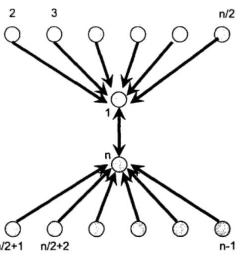
Figure 3-1: The nodes perform an iteration of the nearest-neighbor model with this graph. Every node has a self-loop which is not shown in this picture.

1.

(AG(t)x(t))TQ(AG(t)x(t)) < xTQx, (3.1)

for all connected graphs G on n vertices. 2.

1TQ1 = 0,

where 1 is the column vector of all ones.

Idea of proof: Before jumping into the proof, let us briefly describe the main idea.

1. Suppose we want to show that the sample variance, defined by, U2_{(t) =}

-• in(Xi(t)

x(t))2, where (t) = (1/n) EZI xi(t), is not a Lyapunov function. Consider

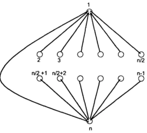
an initial vector x(O) defined by xi(O) = 1, z,,(0) = -1, Zk(0) = 0 for k =

2 .. ..

,-

of the equal neighbour iteration on the graph of Figure 3-1 (note that the graph

d(oes not show self-loops, which are actually present at each vertex). After the

iteration, we will have xl(1) = 1 (1 + (-1) + 0 + ... ·- 0) = 0 and

simi-larlY .r,,(1) = 0. However, x.(1) = (1/2)(1 + 0) = 1/2 for k = 2..., n/2 and,

We now see that the sample variance increased from time 0 to time 1: a2(0) = 2 while a2(1) = (1/4)(n - 2) so that for n > 10, a2_{(O) < a}2_{(1). This shows that}

the sample variance cannot be a Lyapunov function.

2. Let us now show that no diagonal Lyapunov function is possible. A diagonal Lyapunov function is of the form L(x) = xTDx, where D = diag(d11, d22, ... , dn).

It must be that L(x(O)) > L(x(1)) for the x(0) and x(1) we have computed in item 1. Writing this out explicitly,

1

dll

+

dnn > -

Z

dkk-kE{1,2,...,n}-{1,n}

We next derive a similar equation for the sum di, + djj where I now is any index in {1,.. ., n/2} and J is any index in {n/2 + 1,..., n}. Recall that our choice of x(0) and the starting graph of Figure 3-1 is completely arbitrary. For any I E {1,...,n/2} and J

C

xz(0) := 1, xj(0) = -1, and Zk(0) = 0 for k ý {I, J}. We pick a corresponding graph by switching vertices 1 with I and n with J in the graph of Figure 3-1. Then, the analog of the above equation is,

dik + dj 4 1 { dkk. (3.2)

kE{1,2,...,n}-{I,J}

In other words, dl1 + d± j must be large relative to Eke{l,2,...,n}-(I,J} dkk. But

this must hold for all d1, and d .j! We will derive a contradiction from this fact.

Indeed, let us sum Eq. (3.2) over the (n/2)2 ways to pick I C {1, .., n/2} and.

J

C

{rn/2 + 1,...,n}.

(a) Let i E

{1,...,

sum the left hand side of Eq. (3.2) over all possible choices I E { 1 .... rt/2} and J E

{n/2

J. Similarly, i > n/2 + 1, then dii will appear when J = i; there are n/2 such choices as well, exactly one for J and any of the n/2 possibilities for

I.

(b) Similarly, each dii will appear (n/2)(n/2 - 1) times on the right. Indeed, if

i < n/2, then dii will appear on the right if I -i; there are (n/2)(n./2 - 1)

suich choices. Similarly, if i > n/2, then dii will appear on the right if

J : i, which happens (n/2)(n/2 - 1) times. Thus, performing the summation, we have,

(n/2)tr(D) > -(n/2)(n/2 - 1)tr(D).

4

Because D is nonnegative definite, we have that dii 2 0 for all i. Therefore,

because D is nonzero, we have that tr(D) > 0. Canceling (n/2)tr(D) from both sides,

1

1

>

-(n/2

_{- 1),}

-4

which is a contradiction when n > 10.

We next generalize this proof to the case of arbitrary quadratic Lyapunov func-tions.

Proof:

1. Using

the

Q

as,

jij -=0.

i=1 j=1

2. Once again, we begin with the vector x(0) defined by Xi (0) = 1. x,,(0) = -1,

graph G of Figure 3-1 ', the result is xz(1) = 0, , (1) = 0, x2(1). - /2(1)

1/2, x,,/2+1(1) ,....x.,,_(1) = -1/2. By Eq. 3.1, we obtain

f e Qxo xf

Qx

Writing this out in terms of the elements of the matrix Q,

E2, qij +

jE 2,...,n/2} i,j{n/2+1,...,n-1}

qij].

n/2+1,...,nj}-{n}

3. However, our choice to assign initial values of xi(0) = 1 to nodes 1 and n was

completely arbitrary. Let us say we pick nodes I, J instead with x1(0) = 1 and

xj(0) := -1 and disjoint sets AI, Aj each containing n/2 elements with I E A,

and J E Aj. We assign Xk = 0 for k < {I, J}. Then, the analog of the above inequality is: 1 qii + qjj - 2qj > 4( qij + Si,jEAI-{I} _i,jEAj-{J} qij - 2 iEAr-{ I},jEAj-{ J}

4. Let us sum this equation over the (n2 ways to select the two sets A, and Aj

and the (n/2)2 ways to select I and J once AI, Aj are given.

(a) To perform this sunmation, we note some basic combinatorial identities. Given nodes i.j the number of partitions {A!, A. } of {1,.... n} where

i,

j

{A, AI } where one of i.

j

1_{Formally, this is the undirected graph on n vertices made of the edges (1, i) I i= 2...n!2}.}

{(n, i) = 72 n/2 + 1. . .. - 1}. and {(1. n)}. and self-loops { (i. i) i = 1 .. n}

1 q11 + qnn - 2qln > ₄- [ -2 i qij). (3.3)

\ \

2--1

(b) Let us sum the left hand side, which is qli + qJJ - 2qlj, over all possible

ways to choose AI, A , I, J.

i. Each choice of A&, Aj may be followed by (n/2) (n/2) possible choices of I E A, J E Aj. This means each term qii appears n/2 times for each choice of AI, Aj (indeed, i will be in one of the sets - say it is set

AI - and every choice of j E Aj will contribute a qii to the sum). ii. Let us now count how many times the term qij appears in the sum when

i =ý

j.

Q

so that we can write q11 + qjj - 2qij = qui +

qjj

latter representation, we can see that the term qij with i = j appears exactly once with a negative sign in every choice of A&, Aj where i,

j

iii. Therefore, the left hand side sums to

n n-2

n (n/2)tr(Q) - 2 ( 2 1) E qj.

n/2)

_{(n/2 - 1 si}

(c) Similarly, let us consider how often each entry of the matrix Q appears when we sum the right hand side of Eq. (3.3). The right hand side of Eq.

(3.3) is 1 i,jEAI-{I} qij -+ i,jEAj -{J} qij - 2 iEAI-{I},jEAj-{J}

Now each qij is included with a sign of +1 for every distinct choice of A[, Aj, I, J when i i I and i

#

choices. On the other hand, qij appears with a coefficient of +1 for every choice of I, J, A&, Aj where i,

j

j}

(0,

and --1 for every choice where i,

j

}

l{

0.

('n/2

coef-ficiet of -1 is 2 /2 1)2

Therefore. the right hand side sums to 1 nr n-2 1 [n (n/2 - 1)(n/2)tr(Q) + (2(n/2 - 2)(n/2)

4 n/2

(n/2

Putting this all together, we have the inequality:

n/2 (n/2)tr(Q) -(n-2 n/2 -

Z

qij

1Žn

4 n/2)

2

(n/2 -2

-2(n/2

- 1)2

E

qij.

5. But since Ei,j qij = 0, it follows that for real numbers a, 3 it holds that atr(Q)

-3 E~j qij = (a + P)tr(Q). Therefore, we can rewrite the above inequality as:

+ 2 n2 tr(Q)

(n/2 - 1))

If tr(Q) = 0 then Q = 0 since Q is nonnegative definite. Else, canceling tr(Q) from loth sides and plugging in nr = 12. we get 6048 >

(olltradlict ion.

7560, which is a n2 (n/2)

Chapter 4

Averaging with the agreement

algorithm in fixed networks

The agreement algorithm is not guaranteed to converge to the average. However, a variation of the agreement algorithm which does converge to the average has been proposed in [32]. In this chapter, we design another variation of the agreement al-gorithm for the solution of the averaging problem. Our alal-gorithm avoids a small step-size, which is required in [32] for convergence.

We will show that in the case of fixed networks, a single extra parallel pass of the agreement algorithm is sufficient for the agreement algorithm to compute averages. Moreover, this pass need not be repeated if opinions change but the network remains the same. We describe the details below.

4.1

Using two parallel passes of the agreement

al-gorithm

Given a fixed graph G, define the matrix A by ag. = 1/d(i) for all j e Ni. where di is the cardinality of Ni = {j (j, i) E E}. Consider the iteration p -> pA where p is

sonme row vector with elements summing to one. Since A is the transition matrix of the ra•ndom walk oni the graph, and since the presence of self-loops lnakes the period

of the chain equal to one, we conclude that the iteration converges to the row vector 7 defined by 7r = dilE, where E = Ei di is the total number number of edges, including self-loops. Thus, At converges to a matrix whose rows are all equal to 7r.

Consider next the iteration x -- Ax, which is just the averaging algorithm un-der the equal neighbor model on G. It follows from the discussion in the previous paragraph that,

n n

lim xi(t) M = rizx = dixi/E. (4.1)

t

i=1 i=l

The algorithm for computing the average is as follows. The nodes perform two parallel iterations of the equal-neighbor averaging algorithm. At the first iteration the initial value at the ith node is 1/di. The result, which we will denote by z = n/E will at the end be available at every node. The second iteration (performed in parallel

with the first) sets the initial value at the ith node to xi(O)/di. The result of this iteration is then divided by z. The final result is

E n di xi(O0) 1

n i= E di n i=1

which is the desired average. Note that the value of n need not be known by the nodes in order to execute this iteration.

4.2

Comparison with other results

The following averaging method was proposed in [32]. The nodes first agree on some value c

C

degree dmiax and agreeing on 1/(2d,,ax). The largest degree could be computed by a simple iterative algorithm: at each step, each node takes the maximum of its own degree and that of each of its neighbors. After at most n steps, each node knows the highest degree.

Next, the nodes run the iteration xi(t+l1) = (1-Edi)xi(t)+E C 'e N()-i xj(t). This iteration converges to consensus (using either a Markov chain argument. as above, or as a special case of Theorem 1). In addition,. the sum i Xi (t) renlains co(nstant,

which implies that we have convergence to the exact average.

Compared with the algorithm proposed in this chapter, the algorithm of [32] has the disadvantage of uniformly small step sizes. If many of the nodes have degrees of the order of n, there is no significant theoretical difference between the two algorithms, as both have effective step sizes of 1/n. On the other hand, if only a small number of nodes have O(n) degrees, then the algorithm in [32] will force all the nodes to take small steps, in contrast to the algorithm proposed here. The advantages of the algorithm presented here will be illustrated through simulation experiments in Section 7.1 of Chapter 7.

Chapter 5

Estimates of the Convergence Time

In this chapter, we analyze the convergence time of certain time-invariant variants of the agreement algorithm. We also propose a simple heuristic with a favorable worst

case convergence time.

Let X be the set of vectors whose components are all equal. The measure of convergence that we consider in this chapter is the convergence rate defined as

p = sup lim ( t - 12 1/ (51)

x(O)ýX t-10 Jx(O) - x*f12 (

where we denote x* = limt_+• x(t).

The following proposition is well-known.

Proposition 1: Consider the agreement algorithm with a fixed-coefficient matrix A

satisfying Assumptions 1 and 2 (so that A has an cigenvalue at 1. with multiplicity

equal to 1). Then, p = max J\I, where the maxinunm is taken over all eigenvalues A of A different than 1. If the matrix A is symmnetric. then p = max{ IA2

1

},

5.1

Convergence time for the equal neighbor time

invariant model

For the equal neighbor time invariant model, a bound on the convergence rate was computed in [27].

Theorem 3. ([27]) The convergence rate for the equal-neighbor time invariant model,

for any graph on n vertices, satisfies

p < 1 - n

-Moreover, there exists some y > 0 such that for every n E Z+ _{there exists an n-node}

graph for which

p> 1 -

yn-Let us define the convergence time Tn(E) as the first time such that IIx(tx)-X*Il _{I!x(O)-X*Il•} < e -for t > T,(E). Although in principle one could use any norm to define convergence

time, the infinity norm is particularly suited for the consensus problem. Indeed, the final goal of all of the algorithms described in this thesis is to get a set of agents to agree on a value. Thus, the proper measure of performance is how far the agents are from agreement, i.e. maxi xi(t) - mini x (t). Since this is most naturally bounded in terms of the infinity norm, maxi xi(t) - mini xi(t) 211 x(t) - x(oo)l

|,

Then. the above theorem has the following corollary:

Corollary 2. The convergence time for the equal-neighbor time invariant model, for any graph on n vertices, satisfies

T,(c) < (3/4)n3:log n + (1/2)n' log -.

Proof: Let A be the coefficient matrix of an equal-neighbor time invariant model on sonic fixed graph. Consider a randomn walk on this graphI whichl starts at node i and

moves to each of its neighbors with probability ' (note that the random walk may remain at i because of self-loops). Note that the one-step transition probability of this random walk is A. It is known that for any random walk on a graph (Theorem

5.1

of [25]),

(t) - 7 I < r -pj (5.2)

where Pj (t) is the probability of being at node j after t steps, 7rj is the stationary prob-ability of node j, and p is as defined in the previous section, i.e. max{A2(A), AX(A)}.

Since 1 <_ di and n > dj, we can further write

IP(t)

-

7rjl

•

jp

_.

1jP(t)

-

7rj

I• Vni(1

-

n-3)t.

This implies that for t > (3/4)n3 log n + (1/2)n3 log 2, we have IPj(t) - 7rjl < for all j.

Now A" = limt,, At = 7rT1 (see Chapter 4.1 for a proof of this). Thus for

t > (3/4)n3 log n + (1/2)n3 log 2 we have that

At = A0 + E(E),

where I E •. for all i, j. Thus,

.r(t) - x(oo) = Atx(O) - A'x(O) = E('):r(O).

so that

<

_-2

-IIx

(0)11

< Ecx(O) - Z(00)IKoc

where the last inequality follows because the entries of x(oo) lie in the convex hull of the entries of x(0). q.e.d.

5.2

Symmetric eigenvalue minimization via

con-vex optimization

5.2.1

Problem description

Xiao and Boyd [43] considered the following problem. Given a connected, undirected graph G = (V, 8), minimize p over all symmetric, stochastic matrices A that satisfy

aij - 0 whenever (j, i) V E and 1TA = 1T . This problem arises when a network

designer wishes to choose the weights aij to maximize the convergence rate, subject to the constraints induced by a certain communication topology defined by the graph. For example. the nodes may correspond to sensors which are located somewhere in R2

or R3. A communication constraint may be imposed by the requirement that sensors

can communicate only provided they are within a certain distance of each other. The requirement 1TA = 1T enforces the conservation law

ITx(t + _{1) = 1TAx(t) = 1Tx(t),}

thus ensuring that the average (1/n) E•I xi(t) is preserved throughout the execution of the algorithnn. For any matrix A satisfying these constraints.

lini :(t) = limn At x(O) = _{1 1 T} x(0) = •Z (0) 1,

t t n i=1

so that the final consensus is the average of the initial values. The symmetry require-menrt is introdu(ced in [43] in order to obtain a tractable optimization problenm.

5.2.2

Relaxing the constraints

The averaging problem may still be solved even if the constraint 1TA 5 17" is not satisfied and the matrix A is not symmetric. We now describe the details of a two-step procedure for averaging in these conditions.

Provided that the graph (V, {(i, j) aji > 0}) is connected, the Markov chain with probability transition matrix A will have a stationary distribution 7r (Chapter 6.6 of [18]) and

limnAt = 7T1 = -nrT1.

t n

Because 7r is a left-eigenvector of the matrix A, it can be efficiently computed by the network designer. Moreover, it is easy to see that the connectivity of the graph implies 7ri > 0 for all i.

The two-step procedure for averaging is then as follows. As before, the designer communicates to the nodes the coefficients {aij}; now, however, the designer also communicates niri to node i. In the first step, the nodes of the network scale their initial value as

x(0)

Xnew(0) = X() (5.3)

n7r_i

and execute the algorithm with the vector Xnew. The final outcome is

limx(t) lim

Axnew(0)

=(

(

E-n<0) 1 =

_E

_i(o)

₁

_(5.4)

i=.1 n

_i

_ni.1

which is the vector of initial averages.

5.2.3

Our contribution

In this section, we seek to obtain bounds on p for connected Markov chains on finite graphs. As we have just seen. such Markov chains may be used to solve the distributed averaging problem. By obtaining bounds on p for such chains, we obtain bounds on the speed of a class of distributed averaging algorithms.

matrix A. We show that p may approach zero for arbitrary chains of this type. We use this to motivate a constraint which will result in a class of numerically good algorithms, and bound p for the class of chains which satisfy this constraint. We then provide an extended discussion of the convergence time bounds that result from this approach. Finally, we show that a much simpler way of choosing the coefficients results in the same worst-case convergence time.

5.2.4

Convergence rate on a class of spanning trees

We first describe an elementary way to pick a Markov chain on any graph with p arbitrarily close to zero.

Given an undirected graph G = (V, 9), let T = (V, ST) be a spanning tree of G. Pick any vertex of this tree, and designate it to be the root; we will call this vertex

r. We will use NT(i) to refer to the neighbors of node i in T.

Consider a Markov chain on the nodes of G with the following transition proba-bilities: P(i,j) = 1 if

j

j

Next, we will approximate this (reducible) chain with a sequence of irreducible Markov chains. Consider the following probability assignment: for any nonroot vertex

i, P(i,j) = 1 - E|NT(i)l if j is the parent of i in T, P(i, j) = c if j is the child of

i on the tree, and P(i, i) = E. For the root r, we define P(r, r) = 1 - eINT(r)I and

P(r,j) = E where j

E

elements, in the limit as E --- 0 we have that

p--

0

Thus, picking e small, we can get a Markov chain with p arbitrarily small. This

Markov chain can be used to solve the distributed averaging problem as described in Section 5.2.2.