Constrained and phased scheduling of synchronous data flow graphs for StreamIt language

Constrained and Phased Scheduling of Synchronous Data

Flow Graphs for StreamIt Language

by

Michal Karczmarek

Submitted to the Department of Electrical Engineering and Computer Science

in partial fulfillment of the requirements for the degree of

Master of Science in Computer Science and Engineering

at the

MASSACHUSETTS INSTITUTE OF

December 2002

TECHNOLOGY

@ Massachusetts Institute of Technology 2002. All rights reserved.

Author...

Department of Electrical Engineering and Computer Science

/7

C ertified by ...

Sama/Amarasinghe

Associate Professor

Thesis Supervisor

Arthur C. Smith

Chairman, Department Committee on Graduate Students

MASSACHUSETTS INSTITUTE OF TECHNOLOGY

MAY 1 2 2003

Constrained and Phased Scheduling of Synchronous Data Flow Graphs

for StreamIt Language

by

Michal Karczmarek

Submitted to the Department of Electrical Engineering and Computer Science on October 4, 2002, in partial fulfillment of the

requirements for the degree of

Master of Science in Computer Science and Engineering

Abstract

Applications that are structured around some notion of a "stream" are becoming increas-ingly important and widespread. There is evidence that streaming media applications are already consuming most of the cycles on consumer machines [20], and their use is continu-ing to grow. StreamIt is a language and compiler specifically designed for modern stream programming. Despite the prevalence of these applications, there is surprisingly little lan-guage and compiler for practical, large-scale stream programming. StreamIt is a lanlan-guage and compiler specifically designed for modern stream programming. The StreamIt langauge holds two goals: first, to provide high-level stream abstractions that improve programmer productivity and program robustness within the streaming domain; second, to serve as a common machine language for grid-based processors. At the same time, StreamIt com-piler aims to perform stream-specific optimizations to achieve the performance of an expert programmer. This thesis develops several techniques for scheduling execution of Filters in

StreamIt. The work focuses on correctness as well as minimizing buffering requirements

and stored schedule size.

Thesis Supervisor: Saman Amarasinghe Title: Associate Professor

Acknowledgments

I would like to thank my advisor for infinite patience and guidance. The StreamIt team has been invaluable in both the research and writing. Bill Thies helped me with many initial ideas and literature search. Michael Gordon provided the best testing environment

by writing the front end for our compiler and embedding the scheduler in his RAW backend.

David Maze contributed to the internal compiler framework, and help with our printing of program graphs. Jasper Lin hacked our compiler to no end. Chris Leger, Ali Meli, Andrew Lamb and Jeremy Wong wrote scores of applications which I could use for testing.

I want to thank my officemates and friends for putting up with me and convincing me that there is an end to writing. They were right.

Most importantly, I want to thank my all my family and friends, for helping me get here in the first place, and providing constant support.

Contents

3 General StreamIt Scheduling Concepts 3.1 StreamIt execution model . . . .

3.2 Steady State ...

3.2.1 Minimal Steady State . . . . .

3.2.2 Calculating Minimal Steady Stat

3.3 Initialization for Peeking . . . .

3.4 Schedules . . . .

3.5 Schedule Size vs. Buffer Size . . . . .

4 Hierarchical Scheduling 4.1 Motivation . . . . 4.2 Notation . . . . 4.3 Pseudo Single-Appearance Hierarchical Scheduling . . 4.3.1 Filters . . . . 4.3.2 Pipelines . . . . 4.3.3 SplitJoins . . . . 13 17 17 17 19 19 19 20 21 21 23 23 24 25 27 35 36 36 39 39 42 . . . . 43 . . . . 43 . . . . 44 . . . . 46 e . . . . . . . . . . . . . . . . . . . .

4.3.4 FeedbackLoops . . . .4

5 Phased Scheduling 53 5.1 Phased Scheduling . . . . 53

5.2 Minimal Latency Phased Scheduling . . . . 54

5.2.1 Peeking . . . . 55 5.2.2 Notation . . . . 55 5.2.3 General Concept . . . . 56 5.2.4 Filter . . . . 57 5.2.5 Pipeline . . . . 58 5.2.6 SplitJoin . . . . 61 5.2.7 FeedbackLoop . . . . 63

6 Latency Constrained Scheduling 67 6.1 Messages . . . . 67

6.1.1 Timing . . . . 68

6.2 Example . . . . 69

6.3 Information Buffering Model . . . . 71

6.3.1 Intuition . . . . 71

6.3.2 Information Function . . . . 75

6.4 Latency Constraints and Information . . . . 76

6.4.1 Checking for Messages . . . . 76

6.4.2 Information Buffering . . . . 77

6.4.3 Information Buffering and Latency . . . . 77

6.5 Computing the Schedule . . . . 79

6.5.1 Initialization Schedule . . . . 79

6.5.2 Steady State Schedule . . . . 81

6.6 Example . . . . 82 7 Results 85 7.1 Applications. . . . . 85 7.2 Methodology . . . . 86 7.2.1 Schedule Compression . . . . 86 7.2.2 Sinks. . . . . 86 7.3 Results. . . . . 87 8 Related Work 91

9 Conclusion and Future Work 93

List of Figures

2-1 All StreamIt streams . . . .

2-2 Example of a Pipeline with a message being sent . . . .

3-1

3-2 3-3

Sample StreamIt streams . . . .

An illegal SplitJoin . . . . 4 Filter Pipeline . . . .

4-1 Stream for hierarchical scheduling . . . .

4-2 Sample StreamIt streams used for Pseudo Single-Appearance Hierarchical

Scheduling... ...

4-3 Example of non-shedulable FeedbackLoop . . . .

6-1 Example StreamIt program for latency constrained analysis . . . .

7-1 Buffer storage space savings of Phased

archical schedule. . . . .

7-2 Storage usage comparison . . . .

A-I Diagram of Bitonic Sort Application .

A-2 Diagram of CD-DAT Application . . .

A-3 Diagram of FFT Application . . . . .

A-4 Diagram of Filter Bank Application

A-5 Diagram of FIR Application . . . .

A-6 Diagram of Radio Application . . . . .

A-7 Diagram of GSM Application . . . . . A-8 Diagram of 3GPP Application . . . . .

A-9 Diagram of QMF Application . . . . . A-10 Diagram of Radar Application . . . . A-11 Diagram of SJYPEEK-1024 Application

A-12 Diagram of SJYPEEK_31 Application .

A-13 Diagram of Vocoder Application . . .

Minimal Latency schedule vs.

Hier-. Hier-. Hier-. Hier-. Hier-. Hier-. Hier-. Hier-. Hier-. Hier-. Hier-. Hier-. Hier-. Hier-. Hier-. Hier-. Hier-. Hier-. Hier-. Hier-. Hier-. 88 . . . . 89 . . . . 96 . . . . 97 . . . . 98 . . . . 99 . . . . 100 . . . . 10 1 . . . . 102 . . . . 103 . . . . 104 . . . . 105 . . . . 105 . . . . 106 . . . . 106 18 22 28 33 37 40 43 48 69

List of Tables

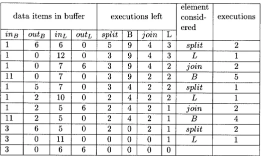
4.1 _{Execution of Steady-State algorithm on sample FeedbackLoop . . . . 51}

5.1 Trace of execution of Minimal Latency Scheduling on a Pipeline . . . . 60

5.2 Execution of Minimal Latency Scheduling Algorithm on a SplitJoin . . . . 62

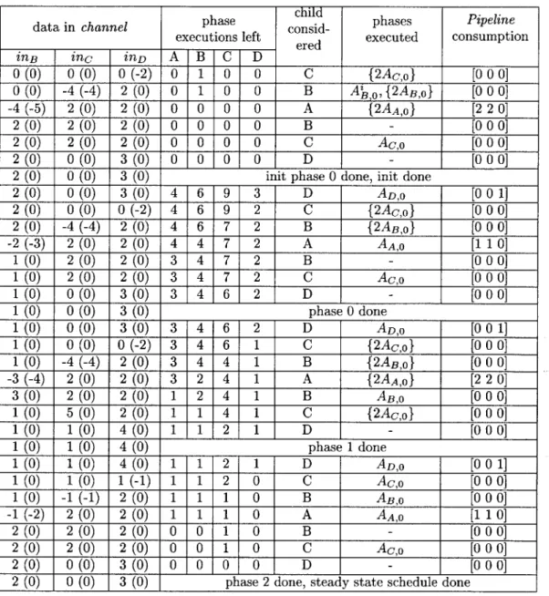
5.3 Execution of Minimal Latency Scheduling Algorithm on a FeedbackLoop . . 65

6.1 Flow of information wavefronts between Filters B an dF in Figure 6-1 . . . 72

6.2 Flow of information wavefronts between Filters A and G in Figure 6-1 . . . 73

6.3 Information per data item in buffers . . . . 76

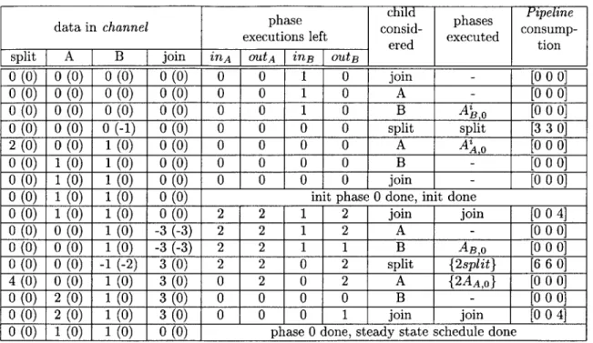
6.4 Sample solution to equations from Section 6.2 . . . . 84

7.1 Results of running pseudo single appearance and minimal latency scheduling

Chapter 1

Introduction

Applications that are structured around some notion of a "stream" are becoming increas-ingly important and widespread. There is evidence that streaming media applications are already consuming most of the cycles on consumer machines [20], and their use is continu-ing to grow. In the embedded domain, applications for hand-held computers, cell phones, and DSP's are centered around stream of voice or video data. The stream abstraction is also fundamental to high-performance applications such as intelligent software routers, cell phone base stations and HDTV editing consoles.

Despite the prevalence of these applications, there is surprisingly little language and compiler for practical, large-scale stream programming. The notion of a stream as a pro-gramming abstraction has been around for decades [1], and a number of special-purpose stream languages have been designed (see [22] for a review). Many of these languages and representations are elegant and theoretically sound, but they often lack features and are too inflexible to support straightforward development of modern stream applications, or their implementations are too inefficient to use in practice. Consequently most programmers turn to general-purpose languages such as C or C++ to implement stream programs.

There are two reasons that general-purpose languages are inappropriate for stream pro-gramming. Firstly, they are a mismatch for the application domain. That is they do not provide a natural or intuitive representation of streams thereby having a negative effect on readability, robustness, and programmer productivity. Furthermore, general-purpose lan-guages do not communicate well the inherent parallelism of stream computations. Secondly, general-purpose languages are a mismatch for the emerging class of grid-based architectures

[17, 25, 21].

StreamIt is a language and compiler specifically designed for modern stream

program-ming. The StreamIt langauge holds two goals: first, to provide high-level stream abstrac-tions that improve programmer productivity and program robustness within the streaming

domain; second, to serve as a common machine language for grid-based processors. At the same time, StreamIt compiler aims to perform stream-specific optimizations to achieve the performance of an expert programmer.

In order to achieve these goals, StreamIt provides a number of features, designed to allow the programmer to easily and naturally express the required computation, while keeping the program easy to analyze by a compiler: all StreamIt streaming constructs are single-input, single-output; all computation happens in Filters; data is passed around between

Filters using three streaming constructs: Pipeline, which allows stacking of Filters one after

another, SplitJoin, which allows splitting and joining of data amongst multiple streams, and FeedbackLoop, which constructs cyclic streams. In StreamIt, every Filter must declare the rate at which it processes data: how much data is consumed and produced on every invocation of the Filter's work function. This model of data passing is called Synchronous

Data Flow (SDF).

In addition to SDF, StreamIt allows the programmer to pass data between Filters in an asynchronous manner, similar to a combination of message passing and function calls. Timing of such data delivery is expressed in terms of amount of information wavefronts

- the programmer can specify a delay between message delivery and destination Filter's

processing of data currently being produced or consumed by the source Filter. Such timing mechanism introduces latency and buffering constraints on execution of StreamIt programs.

Using the features present in StreamIt, the programmer can express complex algorithms and computation models. One of the difficulties faced by StreamIt is scheduling of the execu-tion of the program. Since StreamIt uses SDF computaexecu-tion model with latency constraints, it is possible to schedule the order of execution of Filters at compile time. Scheduling SDF programs presents a difficult challenge to the compiler: as the complexity of the program grows, the amount of memory required to execute the program increases. This increase comes from two sources: the schedule size is creases, as well as amount of data needed for buffering increases. These two sources are closely coupled. There exist tradeoffs between the schedule size and the buffer size.

This problem is further complicated by message latency constraints placed on the pro-gram by the propro-grammer. While StreamIt propro-grams are meant to provide relatively lax latency requirements, it is possible to write programs with latency constraints so tight that very few valid schedules exist. Finding these schedules is a challenging task.

This thesis develops several techniques for scheduling execution of StreamIt programs. This thesis will present techniques which take advantage of structure of StreamIt to create compact schedules. These schedules will be purely hierarchical in nature. The concept of a phasing schedule will be introduced to reduce the requirement for buffering data between

programs with message latency constraints will be solved using integer programming. The contributions of this thesis are:

" hierarchical scheduling of streaming application, a concept enabled by StreamIt

lan-guage,

" first formal handling of SDF graphs with peeking,

* novel phasing scheduling technique,

" a minimal latency schedule using hierarchical phases,

" novel SDF program abstraction called the information buffering model that simplifies

information latency analysis,

" a solution to scheduling of StreamIt programs with latency constraints.

The remainder of this thesis is organized as follows: chapter 2 describes relevant StreamIt constructs in detail; chapter 3 explains basic concepts in scheduling StreamIt graphs; chap-ter 4 describes hierarchical phasing techniques; chapchap-ter 5 describes phasing scheduling tech-niques, including phased scheduling, a more advanced approach to scheduling; chapter 6 introduces techniques for scheduling of StreamIt programs with latency constraints; chapter

Chapter 2

StreamIt Language

This chapter introduces relevant constructs of the StreamIt language. Syntax is not explored here, as it is not relevant to StreamIt scheduling.

Section 2.1 introduces the structured streaming concept, while Section 2.2 introduces the low bandwidth messaging semantics of StreamIt.

2.1

Structure

Perhaps the most distinguishing feature of StreamIt language is that it introduces structure to the concept of stream computation. StreamIt concept of structure is conceptually similar to structured constructs in functional languages such as C.

In StreamIt programs are composed out of streaming components called streams. Each stream is a single-input, single-output component, possibly made up of a hierarchical com-position of other streams. Streams can only be arranged in a limited number of ways, using Pipelines, SplitJoins, and FeedbackLoops. Data passed between Filters is read from and written to channels. Figure 2-1 contains examples of various StreamIt streams. The restrictions on arrangement of streams enforces the structure imposed by StreamIt.

2.1.1 Filters

The basic unit of computation in StreamIt is the Filter. The central aspect of a filter is the

work function, which describes the filter's atomic execution step. Within the work function,

the filter can communicate with its neighbors using the input and output channels, which are typed FIFO queues declared during initialization of a Filter. Figure 2-1(a) depicts a

Filter.

Filters also have the restriction of requiring a static amount of data to be consumed

P₀

peek, pop p

filter

push

(a) A Filter

(b) A Pipeline with n children.

splitter

joiner

(c) A SplitJoin with n children

Filter F upon execution of its work function is called a push amount, denoted push. The

amount of data consumed from input channel by a Filter F upon execution of its work function is called a pop amount, denoted pop. Filters may require that additional data be available in the input channel for the Filter to examine. This data can be read by the

Filter's work function, but it will not be consumed, and will remain in the channel for the

next execution of the work function. The amount of data necessary on the input channel to execute Filter's work function is called peek amount, denoted peek. Note, that for all

Filters peek >= pop. Extra peek amount is the amount of data required on by the Filter

that will be read but will not be consumed, namely peek - pop. The peek, pop and push

values in Figure 2-1(a) correspond to the peek, pop and push amounts of the Filter's work function.

A Filter can be a source, if it does not consume any data, but it produced data. Namely,

a Filter is a source if it has peek = pop = 0. Likewise, a Filter can be a sink, if it consumes

data, but does not produce any, or push = 0.

2.1.2 Pipelines

Pipelines are used to connect StreamIt structures in a chain fashion: each child stream's

output is the next child stream's input. Pipelines have no work function, as they do not perform any computation themselves. Pipelines are simply containers of other StreamIt structures. Figure 2-1(b) depicts a Pipeline.

2.1.3 SplitJoins

SplitJoins are used to specify independent parallel structures that diverge from a common splitter and merge into a common joiner. There are two types of splitters:

(a) Duplicate, which replicates each data item and sends a copy to each parallel stream, and

(b) RoundRobin (wO,..., w1), which sends the first wo items to the first stream, the next

w1 items to the second stream, and so on. If all wi are equal to 0, all child streams of

the SplitJoin must be sources.

RoundRobin is also the only type of a joiner supported in Streamlt; its function is

analogous to a RoundRobin splitter. Figure 2-1(c) depicts a SplitJoin.

2.1.4 FeedbackLoops

joiner, a body stream, a splitter, and a loop stream. Figure 2-1(d) depicts a FeedbackLoop.

A FeedbackLoop has an additional feature required to allow a FeedbackLoop to begin computation: since there is no data on the feedback path at first, the stream instead inputs data from a special function defined by the FeedbackLoop. The amount of data pushed onto

the feedback path is called delay amount, denoted delayfi, for a FeedbackLoop

f

2.2

Messages

In addition to passing data between Filters using structured streams, StreamIt provides a method for low-bandwidth data passing, similar to a combination of sending messages and function calls. Messages are sent from within the body of a Filter's work function, perhaps to change a parameter in another Filter. The sender can continue to execute while the message is en route. When the message arrives at its destination, a special message receiver method is called within the destination Filter. Since message delivery is asynchronous, there can be no return value; only void methods can be message targets. This allows the

send to continue execution while the message is en route - the sender does not have to wait

for the receiver to receive the message and send a return value back. If the receiver wants to send a return value to the sender, it can send a message back to the sender.

Although message delivery in StreamIt is asynchronous in principle, StreamIt does in-clude semantics to restrict the latency of delivery of a message. Since StreamIt does not provide any shared resources to Filters (including global memory, global clock, etc), the timing mechanism uses a concept of flow of information.

One motivating example for messaging in StreamIt can be found in cell phone processing

application. Modern cellular phone protocols involve a technique called frequency hopping

-the cell phone base station selects a new frequency or channel for -the phone to communicate with the base station and informs the phone of this change. The phone must switch to the new channel within a certain amount of time, or it risks losing connection with the base station.

If the phone decoder application is written in StreamIt, the Filter controlling the antenna

and the Filter which will process control signals are likely far apart, and may not have a simple way of communicating data directly with each other. In StreamIt, the Filter which decodes control signals can simply send a message to the Filter controlling the antenna. The message can be sent with a specific latency corresponding to the timing required by the base station. When the antenna controller receives the message it can change the appropriate settings in the hardware to switch to the appropriate new frequency, without having to wait for the appropriate time. The timing of delivery is taken care of by StreamIt.

2.2.1

Information Wavefronts

When a data item enters a stream, it carries with it some new information. As execution progresses, this information cascades through the stream, affecting the state of Filters and the values of new data items which are produced. We refer to an information wavefront as the set of Filter executions that first sees the effects of a given input item. Thus, although each Filter's work function is invoked asynchronously without any notion of global time, two invocations of a work function occur at the same information-relative time if they operate on the same information wavefront.

2.2.2 Message Sending

Messages can be sent upstream or downstream between any two Filters. Sending messages across branches of a SplitJoin is not legal. Timing of message delivery uses the concept of information wavefront. The sender specifies that the message is supposed to be delivered with a certain delay of information wavefront. The delays are specified as ranges, [lo, 111,10 5

li. lo and li specify the information wavefront in executions of the work function of the

sender Filter.

If the message is being sent downstream, the sender specifies that the receiver will receive the data just before it sees the information wavefront produced by the sender between lo and li executions of its work function from when it sends the message. If the message is being sent upstream, the sender specifies that the receiver must receive the message just

before it produces an information wavefront the sender will see between lo and l1 executions

of its work function from when it sends the message.

Message sending is meant to be a low-bandwidth method of communication between

Filters. Message sending is not a fast operation and is intended not to interfere with

the high bandwidth StreamIt communication and processing. However, depending on how tight the latency constraints are (both the magnitude of the latency as well as the range), declaring that messages can be sent may slow program execution down considerably.

Figure 2-2 presents an example of a Pipeline in which the last Filter sends a message to

the first Filter. Filter3 sends a message to Filtero. The message is sent with latency [3, 8].

This means that after at least 3 and at most 8 executions of sender's work function, it will see data produced by the receiver just after receiving the message.

Po

Pi

[38

4[3,8]

FE

P3

Chapter 3

General

StreamIt

Scheduling

Concepts

This chapter introduces the general concepts used for scheduling StreamIt programs. Con-cepts presented here are are common with other languages [16] [3] [14].

Section 3.1 presents the StreamIt execution model. Section 3.2 introduces the concept of a steady state and shows how to calculate it. Section 3.3 explains the need for initialization of StreamIt program. Section 3.4 introduces simple notation for expressing schedules while Section 3.5 presents the tradeoff between schedule and buffer storage requirements.

3.1

StreamIt execution model

A StreamIt program is represented by a directed graph, G = (N, E). A node in G is either a Filter, a splitter or a joiner. Edges in G represent data channels. Each node in G takes data from its input channel(s), processes this data, and puts the result on the output

channel(s). Each data channel is simply a FIFO queue.

Each Filter node nf has exactly one incoming edge and one outgoing edge. The incoming edge is referred to as an input channel, while the outgoing edge is called an output channel.

A splitter node n, has exactly one incoming edge (input channel), but has multiple outgoing

edges (output channels). A joiner node has multiple incoming edges (input channels) but only one outgoing edge (output channel).

Each node of graph G can be executed. An execution of a node causes some data to be collected from the node's input channel(s), the data to be processed and the result to be put on the output channel(s). An execution of a node transfers the smallest amount of data

across the node - it is an atomic operation. StreamIt uses a static data flow model, meaning

node's input channel(s) for consumption or inspection, same amount to be consumed from the input channel(s) and same amount of data to be pushed onto its output channel(s).

Each Filter node nf is associated with a 3-tuple (ef, of, uf). These three values represent the rate of data flow for the Filter for each execution. The first value represents the amount of data necessary to be present in its input channel in order to execute the Filter. This is also called the peek amount of the Filter. The second value represents the amount of data which will be consumed by the Filter from its input channel. This is called the pop amount of the Filter. Note, that ef > of. The final value represents the amount of data that will be put on the output channel of the Filter. This is called the push amount of a Filter. The amount of data present in the input channel of a Filter node nf is denoted irf, while data present in the output channel is denoted outf.

Each splitter node n, is associated with a tuple (o,, w,). The first value represents the amount amount of data that will be consumed by n, from its input channel. Thus, in order to execute n,, there must be at least o, data in its input channel. w, is a vector of integers, each representing the amount of data that will be pushed onto a corresponding

output channel of n,. The amount of data present in the input channel of a splitter node n, is denoted in,, while data present in the ith output channel is denoted out,j.

Each joiner node nj is associated with a tuple (wj, uj). The first value is a vector of integers, each representing the amount of data that will be consumed by nj from its corresponding input channels. In order to execute nj, each of its input channels must have at least as much data in it as the corresponding value in wj indicates. uj represents the amount of data that will be pushed by nj onto its output channel. The amount of data present in the ith input channel of a joiner node nj is denoted inji, while data present in the output channel is denoted ins.

A schedule for a StreamIt program is a list of executions of nodes of graph G. The list

describes the order in which these nodes are to be executed. In order for a schedule to be legal, it must satisfy two conditions. The first one is that for every execution of a node, a sufficient amount of data must be present on its input channel(s), as described above. The second is that the execution of the schedule must require a finite amount of memory.

3.2

Steady State

A StreamIt schedule is an ordered list of firings of nodes in the StreamIt graph. Every

firing of a node consumes some data from input channel(s) and pushes data onto the output

channel(s).

One of the most important concepts in scheduling streaming applications is the steady state schedule. A steady state schedule is a schedule that the program can repeatedly

execute forever. It has a property that the amount of data buffered up between any two nodes does not change from before to after the execution of the steady state schedule. This property is important, because it allows the compiler to statically schedule the program at compile time, and simply repeat the schedule forever at runtime. A schedule without this property cannot be repeated continuously. This is because the delta in amount of data buffered up on between nodes will continue accumulating, requiring an infinite amount of buffering space.

A steady state of a program is a collection of number of times that every node in

the program needs to execute in a steady state schedule. It does not impose an order of execution of the nodes in the program.

Not every StreamIt program has a steady state schedule. As will be explained in Section

3.2.2, it is possible for a program to have unbalanced production and consumption of data

in SplitJoins and FeedbackLoops. The amount of data buffered continually increases, and cannot be reduced, thus making it impossible to create a steady state schedule for them. It is also possible that a FeedbackLoop does not have enough data buffered up internally in order to complete execution of a full steady state, and thus deadlocks. Programs without a valid steady state schedule are not considered valid StreamIt programs. In other words, all valid StreamIt programs have a steady state schedule.

3.2.1 Minimal Steady State

The size of a steady state is defined as the sum of all executions of all the nodes in the program per iteration of the steady state.

Definition 1 A steady state of stream s is represented by vector m of non-negative integers.

Each of the elements in m represents the number of times a corresponding node in s must be executed in the steady state.

Note that m does not impose an order of execution of nodes. Size of a steady state is the total number of executions of all the nodes in the steady state, and is represented by

Ei mi.

Next we will summerize the properties of schedules prsented in [15].

Theorem 1 (Minimal Steady State Uniqueness) A StreamIt program that has a valid

steady state, has a unique minimal steady state.

Proof 1 (Minimal Steady State Uniqueness) Assume that there are two different

min-imal steady states with same size. Let m and q denote vectors representing the two steady states. Let >j mi denote size of schedule m and

E>

that since both m and q are minimal steady states, Ej mi = EZ qi. Since the schedules are

different, there must be some j for which mj = qj. Assume without loss of generality that mj < qj. Since a steady state does not change the amount of data buffered between nodes, the node producing data for node i must also execute less times than corresponding node in q. Similarly, the node consuming data produced by node j also must execute less times than the corresponding node in schedule q. Since a StreamIt program describes a connected graph, it follows that Vi, mi < qi. Thus EZ mi =A Ej qi, which is a contradiction. Thus there cannot be two different minimal steady state.

Corollary 1 (Minimal Steady State Uniqueness) The additional property we have from

the above proof is that if m represents a minimal steady and q any other steady state, then

Vi, mi < qi.

Lemma 1 (Composition of Steady Schedules) If m and q are two steady states for a StreamIt program, then m

+

The above lemma is true because neither m nor q change the amount of data buffered in the channels. Thus a composition of the steady states does not change the amount of data buffered in the channels, which makes the composition also a steady schedule.

Corollary 2 (Composition of Steady Schedules) If m and q are two steady states,

and Vi, mi > qi, then w = m - q is also a steady state.

If q is a steady state and m = w + q is a steady state, then w must not change the

amount of data buffered in channels. Thus w must be a steady state.

Theorem 2 (Multiplicity of Minimal Steady States) If a StreamIt program has a

valid steady state, then all its steady states are strict multiples of its minimal steady state.

Proof 2 (Multiplicity of Minimal Steady State) Assume that there exists a steady

state that is not a multiple of the minimal steady state. Let m denote the minimal steady state. Let q denote the other steady state. Note that w = q - m is still a steady state, as long as all elements of w remain non-negative (by Corollary 2). Repeat subtracting m from q until no more subtractions can be performed without generating at least one negative

element in vector w. Since q is not a multiple of m, w = 0. But since we cannot subtract m from w any further, 31,mi > wi. Since m is a minimal steady state and w is a steady state, this is impossible due to Corollary 1. Thus there are no steady states that are not

3.2.2

Calculating Minimal Steady State

This section presents equations used for calculating minimal steady states. Minimal steady

states are calculated recursively in a hierarchical manner. That is, a minimal steady state is calculated for all children streams of Pipeline, SplitJoin and FeedbackLoop, and then the schedule is computed for the actual parent stream using these minimal states as atomic executions. This yields a minimal steady state because all child streams must execute their steady states (to avoid buffering changes), and all steady states are multiples of the minimal steady states (per Theorem 2). Executing a full steady state of a stream is referred to as "executing a stream".

Notation of Steady States

In this section, the notation for peek, pop and push will be extended to mean entire streams in their minimal steady state execution. That is, a Pipeline p will consume op data, produce uP data and peek ep data on every execution of its steady state. Again, in the hierarchi-cal view of StreamIt programs, a child stream of a Pipeline will execute its steady state atomically.

A steady state of a stream s is represented by a set S, of elements, Ss = {m, N, C, V}.

The set includes a vector m, which describes how many times each StreamIt node of the stream will be executed in the steady state, a corresponding ordered set N which stores all

the nodes of the stream, a vector c, which holds values [e8, os , u.] for stream s, and a vector

v which holds number of steady state executions of all direct children of s. m and v are

not the same vector, because m refers to nodes in the subgraph, while v refers only to the direct children, which may be Filters, Pipelines, splitters and FeedbackLoops.

For a stream s, set S is denoted as S, and the elements of S, are denoted as 5

s,m, 5_s,N,

Ss,candSs,V.

Note, that a steady state does not say anything about the ordering of the execution of nodes, only how many times each node needs to be executed to preserve amount of data buffered by the stream.

Filter

Since Filters do not have any internal buffering, their minimal steady state is to execute the Filter's work function once. This is the smallest amount of execution a Filter can have.

A 3 3,2 B 3 2,2 C 1

(a) A sample Pipeline

3

splitter

A

B

(b) A sample Split Join

2,3

joiner

B

L

splitter

(c) A sample FeedbackLoop. The L Filter has been flipped

upside-down for clarity.

peekL = POPL = 5,pushL = 6 Figure 3-1: Sample StreamIt streams

Sf

=

[1],{f},

[

ef

of

Uf

I

,[]

Notice that Sf,, is empty, because a Filter does not have any children.

Pipeline

Let the Pipeline p have n children and let pi denote the ith child of the Pipeline (counting from input to output, starting with 0, the children may be streams, not necessarily Filters). We must find Sp.

We start with calculating all Spi, i E {0,..., n - 1}. This task is achieved recursively. Next we find a fractional vector v" such that executing each pi 0l' times will not change the amount of data buffered in the Pipeline and the first child is executed exactly once. Since the children streams are executed fractional amount of times, we calculate the amount of data they produce and consume during this execution by multiplying Spi,co and Spi,C, by

v2'. Thus v" must have the following property

We compute v" as follows. The first child executes once, thus v' = 1. The second child

must execute v' = c times to ensure that all data pushed on the the first channel is

P1

consumed by the second child. The third child must execute v' = v'i'p- ₂ - P Up- times to

OP2 _{OP1 OP2}

ensure that it consumes all the data produced by the second child. Thus,

V.2

Next we will find an integral vector v' such that executing each pi vo times will not change the amount of data buffered in the Pipeline. v' will be a valid steady state of the

Pipeline.

In order to calculate v' we multiply v" by "_-Z oP3 . Thus

W-1 U i n-1 i-1 n-1

=(

P

)(

j=

1

)

j=

) (j=i+L

Now we find an integral vector v, such that, for some positive integer g, v' = g * v, and

E; vi is minimal. In other words, we find the greatest integer g, such that v' = g * v, with

v consisting of integers. v represents the minimal steady state for pipeline p.

This is achieved by finding the gcd of all elements in v', and dividing v' by g. Thus V'

V _gcd(v')

v represents the number of times each child of p will need to execute its steady state

in order to execute the minimal steady state of p, thus Sp,V = v. v holds a steady state

because amount of data buffered in p does not change, and it is a minimal steady state, because E2 vi is minimal.

We construct set SP as follows:1

V * Spo,m 0 ... -0 Vn-1 * Spn_1,m, Spo,N 0 ... 0 SPn_1,Ni

ePO v *oPO

1

1n-1

I

An example is presented in Figure 3-1 (a). For this Pipeline, we have the following steady states for all children of the Pipeline:

'Here we use symbol o to denote concatenation of vectors and sets. Thus [1 2 3] o [4 5 6] = [1 2 3 4 5 6] and {A B C} o {D E F} = {A B C D E F}.

1 3

SA=

[1],{A},

,[1},

[1],{B},

2

,

3 3

2 5

SC=

[1],{JD},

2 ,[

,

=

[1],{JD},

3 , []

Using the steady states above, we get the following vector v':

(2*2*3) 12

'= (3)(2

*3)

We now calculate g =

gcd(v')

gcd(12,

12 4 v' 1 18 6 3 3 27 9 9 3 Finally, we construct SP:

4SA,r

o

SC,m

1

-1)

Let the SplitJoin have n children and let sji denote the ith child of the SplitJoin (counting from left to right, starting with 0). Let sj8 and sjj denote the splitter and the joiner of the

SplitJoin, respectively. Let w,,i denote the number of items sent by the splitter to ith child on splitter's every execution. Let wj,i denote the number of items consumed by the joiner from the ith child on joiner's every execution. We are computing Ssj.

Next we compute a fraction vector v" and a fraction a" such that executing the splitter exactly once, each child sji v ' times and the joiner a! times does not change the amount of data buffered in the SplitJoin. Again, since v" and a" are fractions, we multiply the steady-state pop and push amounts by appropriate fractions to obtain the amount of data pushed and popped. For convenience we define a' to be the number of executions of the

splitter and set it to 1.

We thus have that each child sji must execute v' = W _osji times. To compute the number

of executions of the joiner, a'!, we select an arbitrary kth child (0 < k < n) and have that

the joiner executes a' - Usk times. 3 Osk Wj,k

Next we compute integer vector v' and integers a, and aj such that executing the splitter a, times, each child sji vo times and the joiner aj times still does not change the amount of

data buffered in the SplitJoin. We do this by multiplying a', v" and a" by Wj,k (r _{-0 osj,).}

Thus we get

as= Wjk

( id

(i/-=n-i * n'j =W' ii- 1 08 \ -rn-1

Wj,k (lrO Osir * = Ws,i * Wr (H=r Os lr=i+1 oSr

I (n-1, ₁ ' jUj (k1 I (n-1

a' = Wj,k ki0rosr * Wk = s,k * US * '"r=O "Sr r-k+1 OSr

Now we use v', a' and a' to compute minimal steady state of the SplitJoin. Since v',

a' and a' represent a steady state, they represent a strict multiple of the minimal steady

state. Thus we find the multiplier by computing g, the gcd of all elements in v' and integers a' and a', and dividing v', a' and a' by g. We have that

g= gcd(v', _{a' , a'.)}

9 9

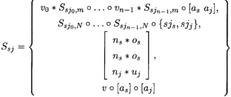
Finally, we use v, as and a3 to construct S,:

V0 * Ssjo,m 0 ... 0 Vn-- * Ssjn1,m 0 [as aj,]

Ssjo,N 0 ... 0 sjin-1,N 0 {sis, s8jI,

ns* o

ns *os ,

U, * U₃

J

V 0 [as] o [aj]

SplitJoin's children:

2 3

SA=

[1],{A},

2

]D

,

[1],{B},

2[

, [

1 6

For this SplitJoin, we select k = 0 (we use the left-most child to compute a['). We get the

following v', a' and a

v'

2 *

1* 2(2) 4

a' = 1* 2(2*2) =8

a = 2* 1(2*2) =8

Thus gcd(u', a', a;) = gcd(8, 4, 8, 8) = 4. Now we obtain

V V 8 2 a'. = a, = 8 = 2 3 = 4= = Finally, we construct S.g: 2 * Ssjo,m o 1 * Ssji,m o [2 2], Ssjo,N 0 Ssji,N 0 {s ss, sj}, 2 Ssi = 2

1

It is important to note, that it is not always possible to compute a unique v" for all possible SplitJoins. The reason is that unbalanced production/consumption ratios between different children of a SplitJoin can cause data to buffer up infinitely.

Definition 2 (Valid SplitJoin) A SplitJoin is valid iff Vk, 0 < k < n - 1, a"'k = ak

using notation of a,k to indicate that kth child of the SplitJoin was used to compute the value of a.

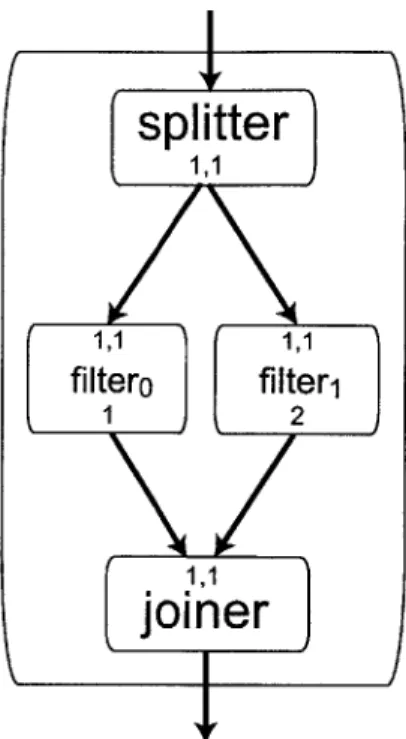
An example of an illegal SplitJoin is depicted in Figure 3-2. The rates of throughput of data for the left child mean that for every execution of the splitter, the joiner needs to

splitter

filtero

filter1

joiner

Figure 3-2: An illegal SplitJoin

be executed exactly once to drain all data entering the SplitJoin. The rates of throughput of data for the right child mean that for every execution of the splitter, the joiner needs to be executed exactly twice to drain all data entering the SplitJoin. That means that consumption of data by the joiner will be relatively slower on the right side, causing data to buffer up. This means that the given SplitJoin does not have a steady state.

If a SplitJoin is such that it does not have a steady state, it is considered an illegal

SplitJoin. It cannot be executed repeatedly without infinite buffering, so a practical target

for StreamIt cannot execute it. The calculations presented here assume that the SplitJoin is legal. In order to check if a given SplitJoin is legal, we test if selecting a different child for calculation of a' yields a different a'J. If it does, then the two paths tested have different production/consumption rates, and the SplitJoin does not have a steady state.

FeedbackLoop

Let FeedbackLoop fl have children B (the body child) and L (the feedback loop child). Let

the joiner and the splitter of the FeedbackLoop be denoted flj and

f

denote the number of data items consumed by the joiner from the input channel to the

FeedbackLoop and from flL, respectively. Let w,,o and Ws,F denote the number of data

items pushed by the splitter onto the FeedbackLoop's input channel and to flL respectively. We are computing Sf1.

First we calculate SB and SL.

Now we compute a fractional vector v" = [a/ a'l a's a'!] such that executing the body

child a" times, the splitter a' times, the loop child a' times and the joiner a' times will not change the amount of data buffered up in the FeedbackLoop. Thus

a/ * uB =a os

a' *uB al*.wj,L

a's8* ,F aL* OB

a * Uj a B* oB

We begin with setting a'! = 1. B needs to be executed "B--j times, the splitter needs₃

OB

to be executed a'' = B times and L needs to be executed a' = g g , times.

OB Os oB o.

Furthermore, in order to assure that the FeedbackLoop has a valid steady state, we continue

going around the loop, the joiner must require WL u = = 1. If this condition is not

OB Os OL Wj,L

satisfied, the FeedbackLoop does not have a steady state. This is a necessary, but not a sufficient condition for a FeedbackLoop to be valid.

Next we compute an integer vector v' = [a' a' a' a'] such that executing B a' times,

splitter a' times, L a' times and joiner a times will not change the amount of data buffered

in the SplitJoin. We do this by multiplying v" by OB * Os *

OL-a' = Uj Os OL

aL= Uj UB *Ws,L

aj = OB *Os *OL a. = Uj *UB *OL

We now use v' to compute v = [aB aL as aj], a minimal steady state for the

Feed-backLoop. We do this by finding an integer g, the gcd of all elements in v' and computing

9

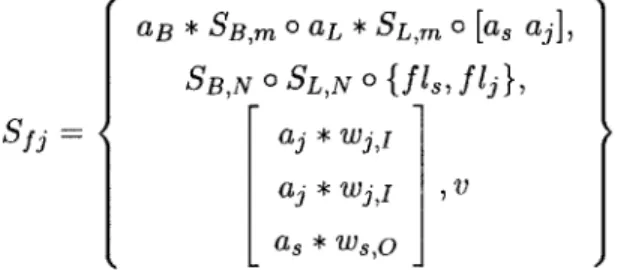
Finally, we construct Sfj as follows:

aB * SB,m o aL * SL,m 0 [as aj],

SB,N 0 SL,N 0

{f

Sfj=

[a

a3 wj,i ,v

[

J

SplitJoin's children:

2 5

SB = [1], {B}, 2 ,U [] SL = [1], {L}, 5 ,0[

1 6

We compute v' for this FeedbackLoop:

5 * 3 * 5 ~ 75~ / 5 * 1 * 3 15 5 * 1 * 5 25 2 * 3 * 5 30 Thus g = gcd(75, 15,25,30) = 5 and 15 1 3 v = -5 ₅ 6 Finally, we construct Sf1 15 * SB,m o 3 * SL,m o [5 6], SB,N 0 SL,N 0 Ifls, flj}, Sfi = 6* 15 3 6* 2 , 5* 3 L 6 _1

3.3

Initialization for Peeking

Consider a Filter f, with peek amount of 2 and a pop amount of 1. When a StreamIt program is first run, there is no data present on any of the channels. This means that for

the first execution, filter

f

After the first execution of f, it will have consumed one data item, and left at least one

data item on its input channel. Thus in order to execute

f

extra data item needs to be pushed onto f's input channel. The same situation persists for

all subsequent executions of

f

This example illustrates that first execution of a Filter may require special treatment. Namely, the source for Filter's data may need to push more data onto Filter's input channel for Filter's first execution. Due to this condition, a StreamIt program may need to be initialized before it can enter steady state execution.

There are other constraints (latency constraints) which may require more complex ini-tialization. These will be discussed in Chapter 6.

After an execution, a Filter

f

Thus, if the only constraints on initialization are peek-related, it is a sufficient condition for

entering steady state schedule that Vf E Filters, inff > ef - of.

Specific strategies for generating initialization schedules for peeking will be presented in Chapter 4 and Chapter 5.

3.4

Schedules

Once a program has been initialized, it is ready to execute its steady state. In order to do this, a steady state schedule needs to be computed. The steady states computed above do not indicate the ordering of execution of the nodes, only how many times the nodes need to be executed.

A schedule is an ordering of nodes in a StreamIt streams. In order to execute the

schedule, we iterate through all of its nodes in order of appearance and execute them one

by one. For example in order to execute schedule {ABBCCBBBCC} we would execute

node A once, then node B, node B again, C two times, B three times and C twice again, in that order.

In order to shorten the above schedule we can run-length encode it. The schedule

becomes {A{2B}{2C}{3B}{3C}}.

3.5

Schedule Size vs. Buffer Size

When creating a schedule, two very important properties of it are schedule size and amount of buffering required. Schedule size depends on encoding the schedule in an efficient way, while amount of space required depends only on order of execution of nodes. The two are related, however, because order of execution of Filters affects how efficiently the schedule can be encoded.

For example, execution of Filters in Pipeline depicted in Figure 3-3 can be ordered in two simple ways, one resulting in a large schedule but minimal amount of buffering, the other resulting in a small schedule but a large amount of buffering.

1,1 A 3 2,2 B 3 2,2 C 1 3,3 D

Figure 3-3: Sample 4 Filter Pipeline. This Pipeline is the same as one in Figure 3-1 (a), except that its children do not peek extra data

times, Filter C 9 times and Filter D 3 times. Writing out a schedule that requires minimal

buffering results in schedule {AB{2C}BCDAB{2C}ABCDB{2C}ABCD}. This schedule

requires a buffer for 4 data items between Filters A and B, 4 items between B and C and 3 items between C and D, resulting in total buffers size 11, assuming data items in all buffers require the same amount of space. The schedule itself has 18 entries.

To compare, writing the schedule in the most compact method we get

{4A}{6B}{9C}{3D}

This schedule requires a buffer for 12 data items between Filters A and B, 18 items between

B and C, and 9 data items between C and D, resulting in total buffers size 39. The schedule

has 4 entries.

We can compare the storage efficiency of these two schedules by assuming that one data item in a buffer requires x amount of memory and each entry in a schedule requires

y amount of memory. Thus the two schedules will require the same amount of storage to

store themselves and execute if IIx + 18y = 39x + 4y.

11x + 18y = 39x + 4y

14y = 28x

y = 2x

Thus the smaller schedule is more efficient if every data item requires less than twice the amount of storage than every entry in the schedule.

One of the difficulties in scheduling StreamIt programs lies in finding a good set of trade-offs between schedule size and buffering requirements.

Chapter 4

Hierarchical Scheduling

In this chapter we present Hierarchical Scheduling, a technique which is quite effective for scheduling StreamIt programs, but which cannot schedule all programs, and which may require the buffers to be very large.

Section 4.1 provides some motivation for hierarchical scheduling. Section 4.2 presents the notation used for hierarchical notation. Section 4.3 provides an algorithm for computing hierarchical schedules.

4.1

Motivation

As has been explained in Section 3.5, the ordering of execution of nodes in a StreamIt program can have a significant effect on the amount of resources necessary to execute the schedule. The two important factors to consider when creating the schedule is amount of buffering necessary to execute the schedule, and the amount of space necessary to store the schedule. The amount of buffering necessary is controlled by the ordering of execution of nodes of the StreamIt graph. The amount of storage necessary to store the schedule is controlled by the encoding of the schedule. As a general rule, ordering which minimizes the buffering space requirements is fairly irregular and difficult to encode efficiently.

One technique used for encoding schedules is to form loop-nests of sub-schedules and repeat them multiple times, until a steady-state schedule is reached. For example, the stream in Figure 4-1 has a following steady state:

6,6 A 4

T

Figure 4-1: A sample stream used for hierarchical scheduling.

9 A 6 C

F

91

2

Thus one steady state schedule for this stream can be

{9{A{2split}{2D}}}{2{{3C}{2split}{2B}}}

Here, {A{2split}{2D}} and {{3C}{2split}{2B}} are the inner nests, executed 9 and 2 times respectively.

If, the overall schedule has every StreamIt node appear only once (as in the example

above), the technique is called Single Appearance Scheduling [7]. One of difficulties in

using Single Appearance Scheduling is finding a good way to form loop-nests for the sub-schedules, because the buffering requirements can grow quite large. An example of this has been presented in Section 3.5.

is possible to use techniques developed for Single Appearance Scheduling to create valid schedules for StreamIt programs, Single Appearance Scheduling does not satisfy all require-ments of an effective StreamIt scheduler. This is because some FeedbackLoops cannot be scheduled using Single Appearance Scheduling techniques. This difficulty arises because the amount of data provided to the FeedbackLoop by the delayfl variable is not sufficient to perform a complete steady-state execution of the loop, thus preventing the schedule for the

FeedbackLoop to be encoded with only a single appearance of every node in the schedule.

The solution to this problem is to have the same node appear multiple times in the schedule. While this solves the problem of inability to schedule some FeedbackLoops, it introduces another problem: which nodes should appear several times, and how many times should they be executed on each appearance. The solution proposed here goes half-way to solve the problem. A more effective solution will be proposed in Chapter 5.

In hierarchical scheduling we use the pre-existing structure (hierarchy) to determine the nodes that belong in every nest. Basically, every stream receives its own loop-nest, and treats steady-state execution of its children as atomic (even if those children are streams whose executions can be broken down into more fine-grained steps). In the exam-ple above, the Pipeline has a SplitJoin child. The SplitJoin is responsible for scheduling its children (nodes C, B, split and join). The Pipeline will use the SplitJoin's

sched-ule to create its own steady state schedsched-ule. Here the SplitJoin's schedsched-ule can be Tj3 =

{{9split}{3C}{9D}{2join}}, thus making the Pipeline's schedule 1

Tpipe = {{9A}{2Tsj}{4B}} = {{9A}{2{{9split}{3C}{9D}{2join}}}{4B}}

The problem of inability to schedule some FeedbackLoops is alleviated by allowing

Feed-backLoop to interleave the execution of its children (the body, the loop, and the splitter and joiner). This results in FeedbackLoop containing multiple appearances of its children. All

other streams use their children's schedules in their schedules only once. This technique is called Pseudo Single Appearance Scheduling, since it results in schedules that are very similar to proper single appearance schedules. While it does not allow scheduling of all

FeedbackLoops (a FeedbackLoop may have a child which requires more data for steady state

execution then made available by the delayfi variable) it has been found to be very effective, and only one application has been found which cannot be scheduled using this technique.