A coupled atmosphere-ocean model of thermohaline circulation, including wind-driven gyre circulation with an analytical solution

(1)

A Coupled Atmosphere-Ocean Model of Thermohaline Circulation, Including Wind-driven Gyre Circulation with an Analytical Solution

by Elise M. Olson

Submitted to the Department of Earth, Atmospheric and Planetary Sciences in Partial Fulfillment of the Requirements for the Degree of Bachelor of Science in Earth, Atmospheric and Planetary Sciences at the Massachusetts Institute of Technology

Februrary 2006

MASCHUT TOTE

OF TECHNOLOGY

OCT 2

4 2017

LIBRARIES

Author-Signature

redacted

Department of Earth, Atmospheric and Planetary Sciences Ma 23 204 Certified by_ Accepted by

igatrereace

Signature redacted

y , Peter H. Stone Thesis Supervisor J. Brian Evans Chair, Undergraduate Thesis Committee The author hereby grants to MIT permission to reproduce and to distribute publicly paper and cectronic cop:s of Lhis thesis document in whole or in part in any medium now known or hereafter created.

(2)

A Coupled Atmosphere-Ocean Model of Thermohaline Circulation, Including Wind-driven Gyre Circulation with an Analytical Solution

by Elise M. Olson

Submitted to the Department of Earth, Atmospheric and Planetary Sciences May 19, 2005

In Partial Fulfillment of the Requirements for the Degree of Bachelor of Science in Earth, Atmospheric and Planetary Sciences

Februrary 2006

Abstract

A parameter representing circulation due to wind forcing is added to the thermohaline circulation model of Marotzke (1996). The model consists of four boxes and is governed by a system of two differential equations governing the temperature and salinity

differences between high latitude ocean and low latitude ocean boxes. The modified model is solved numerically for equilibrium solutions, and then solved analytically by the method of Krasovskiy and Stone (1998). At the maximum strength of wind-forced

circulation studied, v = 5 x 10-" s', a stable thermal mode equilibrium temperature difference of 25 K is calculated. Once v reaches a critical value, which is within the range of physically reasonable values, the stable haline mode equlibrium and unstable thermal mode equilibrium are no longer observed. It is concluded that strong wind-forced circulation suppresses the thermal mode equilibrium, but that more research is necessary to determine the degree to which this effect is present in the real world.

Thesis Supervisor: Peter H. Stone Title: Professor of Climate Dynamics

(3)

Acknowledgements

First, I would like to thank my thesis supervisor, Professor Peter Stone, for his invaluable guidance in this project as well as for everything I learned in his Global Change Science class. In addition, I would like to thank the faculty and staff of the Department of Earth, Atmospheric, and Planetary Sciences, who, in every instance, have been overwhelmingly helpful and inspiring. In particular, I am grateful to Professor Paola Malanotte-Rizzoli for introducing me to the type of box circulation model studied in this thesis through a UROP project. I would like to thank Dr. Kimberly De Vries and Cameron Wobus for their editing help and advice as well as flexibility in scheduling. To Zhenye Mei, thank you for your kindness and understanding and for all the dinners you cooked even though you were as busy as I was. Finally, thank you to my parents, whose support I have come to value even more over the past few years.

(4)

Table of Contents 1. Introduction... 5 2. Literature Review... 7 3. M ethods ... 18 4. Numerical Results ... 20 5. Analytical Solution... 27 6. Conclusions... 34 References ... 35 Figures 1. Diagram of model, adapted from Stommel (1961)...9

2. Four-box model similar to M arotzke and Stone (1995)... 12

3. Six-box Shaffer and Olsen (2001) model... 12

4. Plot of meridional temperature difference vs. wind-forcing parameter, m = n = 1...23

5. Plot of meridional salinity difference vs. wind-forcing parameter, m = n = 1...23

6. Plot of meridional temperature difference vs. wind-forcing parameter, m = n = 3...24

7. Plot of meridional salinity difference vs. wind-forcing parameter, m = n = 3...24

8. Time evolution of T and S, V = 0 ... 26

9. Time evolution of T and S, v = 5 x 101" s-1... 26

10. Time evolution in S-T plane, v = 0... 26

11. Time evolution in S-T plane, v = 5 x 10-1 s-...26

12. Plot of

9

vs. y exhibiting all three equilibrium solutions... 32

13. Plot of y vs. y at g = h...32

14. Plot of vs. yforg > h... 33

Table 1. Parameter values and definitions... 21

(5)

1. Introduction

The factors that contribute to climate variation and their relative importance are not yet well understood, but they are of great interest because of concerns about global warming. Predictions of global temperature increase by current climate models range from small to alarmingly large. Many scientists are therefore interested in discovering how anthropogenic changes to the environment affect climate so that these factors can be effectively integrated into climate models. However, the manner in which climate

change is brought about is not straightforward. Many feedback mechanisms magnify or damp perturbations to the parameters affecting climate, leading to a highly nonlinear and complex system.

Because the factors governing climate are so complex, it is impossible to conduct laboratory experiments isolating each factor in the system. Instead, researchers develop simplified models based on physical mechanisms believed to affect climate. Some of the simplest models consist of boxes representing segments of the ocean and atmosphere between which heat and moisture are exchanged. An important aspect of all such models is the thermohaline ocean circulation driven by density gradients due to differences in temperature and salinity between boxes. The thermohaline circulation is one of the mechanisms that transfer heat and salinity between boxes. These models often have several equilibrium solutions for temperature and salinity, and different equilibrium solutions are expected to correlate with different types of climate. The models are mathematically analyzed to see how changes in various parameters alter the equilibrium solutions, and since the equilibrium solutions are analogous to climate states, insight may be gained into how these mechanisms might affect real climate. Findings from such

(6)

simplified models can be applied to aid in the development of more complex general circulation models, which more directly reflect the behavior of the real climate.

The object of this thesis will be to develop and analyze a four-box coupled atmosphere-ocean circulation model that includes the effect of wind-driven gyre circulation. It will be an extension of a four-box model, developed by Marotzke and Stone (1995), to include a wind-driven circulation term to represent the way wind forcing at the surface of the ocean increases mixing between high and low latitudes in the North Atlantic.

(7)

2. Literature Review

The most sophisticated models used to predict climate change are called general circulation models, or GCMs. These highly complex models are limited not only by current understanding of climate processes but also by available computing power. As

Stone (2004) points out, subgrid-scale processes, uncertainty in how far the current climate is from a bifurcation, and the potential for chaotic behavior all limit the ability to construct accurate models to predict climate change.

Sub-grid scale processes are processes that occur over distances smaller than the spatial resolution that can be achieved using contemporary computers. These processes, such as convection and diapycnal mixing, must be represented by parameterizations that are likely to introduce error into the model. The wind-driven gyre circulation that will be analyzed in this study is a type of diapycnal mixing. The second source of difficulty discussed by Stone arises from the fact that GCMs generally demonstrate more than one equilibrium state for at least some parameter values. How far the current climate may be from a bifurcation where the number of possible equilibrium states changes is unknown, and the stability of the current climate depends strongly on this factor. Third, Stone points out that the characteristics of the climate system are such that its behavior is likely to be chaotic and therefore have inherently limited predictability. However, the scale of this limitation is difficult to assess due to the long timescales over which ocean

circulation adjusts to changes. Thus, a more complete understanding of climate

interactions is necessary to improve GCMs and even to assess the ultimate limitations of climate prediction.

(8)

Simple models can be useful tools to gain insight into the fundamental physical processes at work in the climate system. Stommel's (1961) thermohaline circulation model is one of the simplest and is the precursor to the other models discussed in this paper. First, Stommel (1961) developed a model consisting of a vessel of water and a reservoir through which heat and salt are exchanged at a rate proportional to the differences in temperature and salinity, respectively, between the vessel and reservoir. The vessel is assumed to be uniformly mixed at all times, and the reservoir is assumed to have constant temperature and salinity (Stommel, 1961). If the temperature and salinity in the vessel are T, and S,, and the temperature and salinity in the reservoir are T2 and S2, where T1, S1, T2, and S2 represent deviations from reference values, then the rates of change of temperature and salinity in the vessel can be expressed as follows:

dT

dt = c(T2-T 1), (1)

dS₁ = d(S2 -Si), ₍₂₎

dt

where c and d are constants (Stommel, 1961). Stommel shows that over infinite time, the system reaches the state T,=T2 and S1=S2. Then Stommel (1961) invokes the equation of state,

p = po(1- aT +

PS),

(3)

where p represents the water's density and c and

P

represent the thermal expansion and haline contraction coefficients of seawater, respectively. If, initially, T, = S, = 0, the final density is greater than the initial density when @S2/aT2> 1 (Stommel, 1961).

(9)

return flow q

reservoir vessel a vessel b - reservoir

T2 S2 Ti S1 -T1 -SI' -T2 -S 2

q ) capillary

Figure 1: Diagram of Stommel (1961) model. Direction of flow, q, shown is for salinity driven circulation.

Next, Stommel (1961) expands the model to include a second vessel-reservoir system with T2' = -T2, and S2' = -S 2. The two systems are connected above by an

overflow channel that keeps the surfaces at the same height and below by a capillary tube with resistance k, as shown in Figure 1. If the density of the first vessel is Pa and the density of the second vessel is Pb, both determined by the equation of state (3), then

kq = pa - P, (4)

where q is the flow through the capillary from the first vessel to the second vessel and is balanced by an equal return flow in the overflow channel (Stommel, 1961). The

circulation described by q is driven by a pressure gradient resulting from density

differences. The force of gravity is greater on the denser water than the less dense water. Therefore, if Pa > Pb, the pressure at point a is greater than the pressure at point b, and

water will flow down the pressure gradient, along the capillary from vessel a to vessel b. In order to conserve mass, a return flow must occur. In the diagram, q is shown with arrows in the counterclockwise sense corresponding to Pa > Pb- If Pb > Pa, however, the

(10)

flow is clockwise, and q has a negative value. Stommel derives the following equations based on conservation of temperature and salinity, defining T=T,=-Tl' and S=S=-S₁':

dT

-- = c(T2 - T) -

|2q|T,

(5)

dS

dt= d(S2 -S) -

|2q|S,

(6)

Solving the system of equations formed by equations 4 through 6, Stommel (1961) finds that for some values of the parameters there are as many as three real equilibrium (steady-state) solutions, corresponding to a stable node, a stable spiral, and a saddle. Thus, Stommel (1961) finds that the system can have two stable equilibria- one

corresponding to a temperature-dominated (thermal) mode with negative q and the other to a salinity-dominated (haline) mode with positive q and flow in the sense depicted in Figure 1. The first equilibrium occurs when the density difference due to temperature dominates, and flow is from the low temperature box, 1, to the high temperature box, 2. The second equilibrium occurs when the density difference due to salinity dominates, and the flow through the capillary is from the dense high salinity box, 2, to the low salinity box, 1. Stommel (1961) concludes with the speculation that such "different states of flow" might exist in nature, for instance, in ocean thermohaline circulation, and that sufficient perturbation could cause the system to switch from one type of flow to the other. Because the thermohaline circulation in the North Atlantic transfers heat from the tropics to the poles, its reversal might lead to a climate with a large meridional

temperature gradient and very cold temperatures at high latitudes.

Subsequent papers by other authors aim to gain insight into the physical processes at work in the Atlantic Ocean using similar models. Nakamura, Stone and Marotzke

(11)

(1994) develop a model consisting of two atmospheric boxes and three ocean boxes. The Northern Hemisphere is considered, and the atmosphere and ocean are divided along a line of latitude 35*N. The low latitude ocean is divided into a shallow box and a deep box while a single box represents the high-latitude ocean2_{. An important aspect of the}

model is the coupled atmosphere, allowing feedbacks between sea surface temperature distribution and atmospheric heat and moisture fluxes. Previous models represented heat and moisture fluxes with fixed parameters. Nakamura, Stone and Marotzke (1994) find that the dependence of atmospheric moisture transport on temperature leads to a positive feedback that destabilizes the thermohaline circulation, dubbed the "eddy moisture transport-thermohaline circulation feedback", or "EMT feedback". A reduction in thermohaline circulation leads to an increased meridional temperature gradient, which in turn increases low-latitude evaporation and atmospheric moisture transport. The

increased freshwater flux at high latitudes reduces the meridional salinity gradient, reducing the high-latitude sinking that drives the thermohaline circulation (Nakamura et

al, 1994).

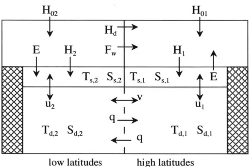
Marotzke and Stone (1995) develop a model along the lines of the Nakamura et al (1994) model but with only four boxes and a simpler parameterization of atmospheric transports, allowing the possibility of an analytic solution. The atmospheric heat and

moisture transports are linearly related to the meridional temperature gradient in this model. The geometry of the model is shown in Figure 2. Marotzke and Stone (1995) find that the coupled atmosphere reduces the range of stable thermal mode solutions due to the EMT feedback as described by Nakamura et al (1994).

2 The geometry of the model can be visualized by combining the high-latitude half of

(12)

H_{0 2}

low latitudes

Hoi

high latitudes

Figure 2: Model similar to Marotzke and Stone (1995), Marotzke (1998), and Krasovskiy and Stone (1996). The parameter v represents wind-driven mixing, the factor added to the model and analyzed in this study.

H_{0 2}

Hoi

low latitudes high latitudes

Figure 3: Shaffer and Olsen (2001) model: atmospheric, surface, and deep ocean boxes

Marotzke (1996) studies feedback mechanisms in a model nearly identical to that of Marotzke and Stone (1995). The major difference is the parameterization of heat and moisture flux, for which a general power law is adopted in place of a linear one. Again,

Hd

H

2

FI

T

HI E

E

q

__

T2S2

D

T1

Si

T2 _{__}

_q

Hd- >

E

H

2

Fw- +

Hi

STs,2

Ss,2

Ts,1

S,,+

E

U2 Ui q Td,2 S d,2

q

TdI Sd,1

(13)

Marotzke (1996) finds that increasing dependence of atmospheric moisture transport on the temperature gradient destabilizes the thermohaline circulation. When the atmospheric moisture transport depends weakly on temperature, decreasing temperature dependence of atmospheric heat transport stabilizes the thermohaline circulation. However, when the atmospheric temperature dependence of the moisture transport is strong, decreasing temperature dependence of atmospheric heat transport destabilizes the thermohaline circulation (Marotzke, 1996).

As the model studied by Marotzke (1996), which is solved analytically by

Krasovskiy and Stone (1997), is the direct precursor to the model that will be used in this study, it is useful to discuss it in some detail. The backbone of the model consists of a set of differential equations for the time rate of change of temperature and salinity in the ocean boxes. The subscript 1 always refers to the high-latitude boxes, and 2 to the low-latitude boxes, as shown in Figure 2.

dT1 HI +ql(T2- TI) (7) dt dT_{-T2= H2- -ql(T2 - TI)}2 8 (8) dt dS- -H, +jqj(S ₂-S1) ₍₉₎ dt dS dS =HS -jqj(S 2 -Si) (10) dt

H, and H2 are the heat fluxes into the ocean boxes, and H, is the virtual salinity flux, which corresponds to net rain in box 1 and net evaporation in box 2. The heat fluxes, H, and H2, are calculated from the net radiation into the atmospheric boxes, HO,

(14)

and H02, and the heat transport between boxes, Hd. The net radiation into each of the atmospheric boxes is

SA BTI,(11) and

H02 = _A2 -BT2. (12)

A, and A2 are the net incoming radiation to the high and low latitude boxes, respectively, if the surface temperature is 0*C. BT, and BT2 represent adjustments that account for changes in the amount of longwave radiation that result from deviations of surface temperature from 0*C. The meridional heat flux, Hd, is parameterized by the equation

Hd = y(T2 -T)", (13)

where n is a constant chosen so that the stable thermal mode solution resembles the

current climate. Thus, if the stable thermal mode solution has T = T2 - T,, then

kii= J . Similarly, the meridional freshwater flux, F, which is used to find H, is

parameterized by the equation

Fw =

im(T

2 -Ti) m1 (14)

where im is a constant, and IT = mm.

Since the particular location of the division between the high-latitude and low-latitude boxes is fairly arbitrary, the areas, Fo1 and F02 of the atmospheric boxes are taken

to be equal, and so are the areas of the ocean boxes, F, and F2. Thus, the ratio of ocean box area to atmospheric box area is

F F

=- 2 (15)

FOI _F₀

(15)

If xn = 5s /Fo0 , then 1 HI = -(HOI _{+ Hd/FI)} ecpOD H2 =- 1

_(H

₀₂ EcpOD - Hd/F1) = = DcPAD - BT, + x.(T2 - TI)" ], sEpoD c A2 - BT2 - X(T2 - TI)" , FIepoD

where c is the specific heat capacity of seawater, po is the mean density of seawater, and D is the ocean depth.

The virtual salinity flux, H, is given by H~E

HS = so

-D (18)

where So is a constant reference salinity and E is the rate of water loss in low latitudes and gain in high latitudes. The moisture flux E is

I F E - F Ew Fol'

(19)

where EW is the ratio of the area of the ocean to the catchment area, the area over which

fallen rainwater flows into the ocean. Thus, if Ym =

Ym/Foi

, then

HS= D= Ym(T₂-T).

S w D F₁ ED

(20)

Finally, the variable T is taken to be T2- T,, and S to be S2 - S1. Then, dT = '(T02 -TO 1 - T) - 21T -2|qlT, dt dS = 2Tm_{T" -2|qS,} dt (21) (22)

where k = B/ccpOD, To, = A1/B, T02 = A2/B, V= Xn/EcpOD, and Fm = SoYm

/F

wD. The

volume flux due to the thermohaline circulation, q, is parameterized as and

(16)

(16)

q = k(T - PS).

Krasovskiy and Stone (1998) analytically solve the model described above and studied by Marotzke (1996). Krasovskiy and Stone (1998) confirm the results of Marotzke (1996) in a more general form and also note that the EMT feedback is a negative feedback in the haline mode. According to Krasovskiy and Stone (1998), it is more realistic for the atmospheric heat and moisture fluxes to depend on the same power of the temperature difference, and increased temperature dependence destabilizes the thermohaline circulation in its current state.

Longworth, Marotzke and Stocker (2004) and Shafer and Olsen (2001) both study the effects of the addition of wind-driven gyre circulation to thermohaline

circulation models. Longworth, Marotzke and Stocker (2004) discuss two models- one based on the Stommel (1961) model, and another, called the Rooth model, with three ocean boxes representing southern high latitudes, tropics, and northern high latitudes. Neither model includes a fully coupled atmosphere such as that of the Nakamura et al (1994) or Marotzke and Stone (1995). In the Stommel model, wind-driven circulation stabilizes the stable thermal mode equilibrium (Longworth et al, 2004). For some parameter values, the model can have two stable equilibrium solutions and one unstable equilibrium solution, as can the original Stommel model. For other parameter values, only the stable equilibrium solution representing high latitude sinking is present due to the reduction of the meridional salinity difference by wind-driven forcing (Longworth et

al, 2004). In the Rooth model, which has no haline mode, wind-driven mixing stabilizes

solutions in which sinking occurs in the hemisphere with larger salinity flux, or weaker freshwater flux (Longworth et al, 2004).

(17)

In addition to adding a wind-driven mixing parameter, Shaffer and Olsen (2001) adapt the Marotzke and Stone (1995) model to include two shallow ocean boxes, for a total of six boxes in the new model, as depicted in Figure 3. In this model, the EMT feedback has virtually no effect. In addition, with values of v estimated for the current climate, the salinity-driven steady-state solution characterized by sinking in the low latitudes is no longer viable (Shaffer and Olsen, 2001). In this model, as in the Stommel model, increased wind-driven horizontal mixing stabilizes the stable thermal mode equilibrium and can eliminate the stable haline mode solution. These results can be explained by the fact that the parameter v does not depend on salinity, and therefore reduces the dependence of circulation on salinity, which is crucial to the EMT feedback as well as the salinity-driven equilibrium solution (Shaffer and Olsen, 2001). The temperature dependence of the circulation is relatively unaffected because the

thermohaline circulation depends more strongly on temperature than on salinity (Shaffer and Olsen, 2001).

In general, the addition of wind-forcing terms to simple box models has reduced the range over which a salinity-driven equilibrium solution with low-latitude sinking can exist. This suggests that in the current climate, mixing due to wind stress may reduce the likelihood of a reversal in the thermohaline circulation. In this thesis, wind-driven gyre forcing will be added to the Marotzke (1996) model, in order to see to what degree the addition of wind forcing changes the behavior of the model when no other aspects of the model are changed. An analytical solution will be sought in order to clearly identify the mechanisms involved.

(18)

3. Methods

The four-box coupled atmosphere-ocean model, as developed by Marotzke (1996) and solved analytically in Krasovskiy and Stone (1998), is here modified to include a term representing wind-driven gyre circulation. The gyre circulation term has the same form as that used by Shaffer and Olsen (2001) in their six-box model and by Longworth

et al (2004) in their models containing ocean boxes without coupled atmosphere. Eqs.

(24) through (27) correspond to Eqs. (7) through (10) in the preceding exposition of the model studied by Marotzke (1996) and Krasovskiy and Stone (1998). These equations relate the time derivatives of temperature and salinity in each box to the heat and freshwater fluxes from the atmosphere and the advection of heat and salt with the flow. The variable v represents an inverse timescale, or volume flux, associated with wind-driven gyre circulation.

dT1 HI + ql(T2- TI)+ v(T2- T,) (24) dt dT2 =H2 -|q|(T 2- T) - v(T2- T) (25) dt dS1 _(6 dt- -H, +ql(S 2 - SO)+ v(S2 -S) (26) dt s

dS

2 = H, - qj(S₂- Si) - v(S₂- Si) (27) dt

Eqs. (28) and (29) are the equivalent of Eqs. (21) and (22) in the original model. Again, the variable T represents the meridional temperature difference and S represents the meridional salinity difference.

dT

-= (T2 -T01 - T) - 2 T - 2|qlT - 2vT, (28)

(19)

dS

--- = 2FmTm - 2JqlS - 2vS, (29)

dt (9

where all variables, excluding the new parameter v, are as defined before.

First, the system is solved numerically for equilibrium solutions using MATLAB, and the stability of the equilibrium solutions is determined. Equilibrium solutions are plotted as a function of v, and sample trajectories in the T-S plane are computed with a Runge-Kutta algorithm for two values of v. Then, the system is solved analytically, using an expansion around the equilibrium states found numerically, by the same method described in Krasovskiy and Stone (1998).

(20)

4. Numerical Results

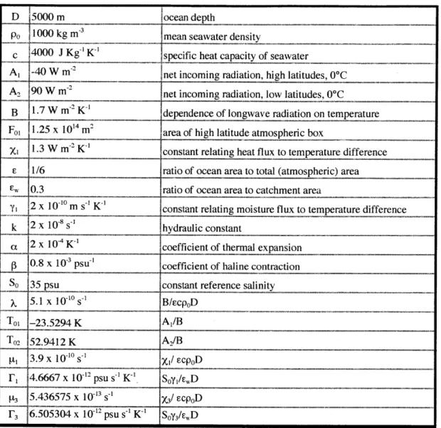
Equilibrium solutions are calculated numerically using the parameter values given in Table 1. The parameter values chosen are those used by Marotzke and Stone (1996), and were chosen so that if v = 0, the stable thermal mode solution is similar to the current climate. Equilibrium solutions consist of pairs of values, (T, S), for which the time derivative of the meridional temperature difference and the time derivative of the meridional salinity difference equal zero. First, the temperature exponents, m and n, in atmospheric flux parameterizations, are both taken to be one. Figures 4 and 5 are plots of the equilibrium temperature and salinity differences between high and low latitude boxes versus the mixing parameter. For each value of v, there is an equilibrium solution

consisting of the temperature difference described by Figure 4 and the salinity difference shown in Figure 5. The mixing paremeter, v, is plotted from zero to 5 x 10-" s-,

covering the range of values considered in Shaffer and Olsen (2001) and Longworth et al (2004).

An ocean that covered one-tenth of the Earth's surface at constant depth of 5000 meters would have a volume of approximately 2 x 10" cubic meters. Therefore, the maximum value of v considered, 5 x 10-" s', corresponds to a flow of approximately 107

cubic meters per second, or 10 Sv3

. A reasonable estimate of the horizontal volume flux due to wind-driven circulation in the current climate is 5 Sv (Shaffer and Olsen, 2001). Here, v = 2.5 x 10-" s' corresponds approximately to 5 Sv.

(21)

D 5000 m Mocean depth

Po 1000 kg mean seawater density

c 4000 J Kg'K' specific heat capacity of seawater

Al -40 W m _{net incoming radiation, high latitudes,}_0*C

A 90 W M-2 _{net incoming radiation,}_{low latitudes,}_0*C

B 11.7_W M-2 K- dependence of longwave radiation on temperature

F1 1.25 x 1014 m 'area of high latitude atmospheric box _ Xi 1.3 W m K- constant relating heat flux to temperature difference

s 1/6 ratio of ocean area to total (atmospheric) area

0.3 _ratio of ocean area to catchment area

2 x 100 m s- K) _{constant relating moisture flux to temperature difference}

k 2 x 10- s hydraulic constant

2 x io-4K' _{coefficient of thermal expansion}

p 0.8 x 10-3 psu- coefficient of haline contraction

So 35 psu constant reference salinity

x

5. 10I4W s-' _ B/__ ~cp₀D To, -23.5294 K Al/B T0 2 52.9412 K A2/B t13.9 x 0 s- _{Xj/ EcpOD} F, 4.6667 x 10-2 psu s K1. Soy1Is D S5.436575 x 10-3 s- X3/ EcpOD F3 6.505304 x 10-12 psu s- K' Soy₃/s₁wD

(22)

As Figures 4 and 5 demonstrate, the stable haline mode equilibrium and the unstable thermal mode equilibrium intersect at v = 1.86 x 10-" s', which corresponds to a wind-driven gyre flow below Shaffer and Olsen's estimate of the ocean's actual circulation at around 5 Sv. As v increases further, only the stable thermal mode equilibrium solution remains. Thus, when the wind-driven gyre circulation is strong enough, the thermal mode solution, corresponding to the high-latitude sinking that characterizes the current climate, is the only possible stable equilibrium. Over the range studied, the wind-mixing parameter reduces the stable thermal mode equilibrium temperature difference by approximately 2 K and salinity difference by approximately 0.5 psu.

Next, the equilibrium temperature differences are plotted versus the mixing parameter for atmospheric transports proportional to the third power of the temperature difference, so that m = n = 3. These plots are shown in Figures 6 and 7. The atmospheric transport parameters, t3 and F₃, are calculated for the v = 0 case, without wind-driven

mixing, and their values are shown in Table 1. The critical value of the mixing

parameter, v, increases slightly, to about 2 x 10-1 s'. In addition, the increased strength of negative feedbacks between atmospheric transports and the temperature gradient destabilizes the thermohaline circulation slightly; in general the critical salinity perturbation necessary to shift the system from the stable thermal mode to the stable haline mode, calculated by finding the difference between the unstable and stable thermal

(23)

Equilibrium Temperature Differences vs. Wind-forcing Paramete: 301 1 H

29.5

28.5

27.5

26.5

25.5 24.5'

0

1 2

v (s-1)

3

4 5 x 10-11

Figure 4: Plot of meridional temperature difference vs. wind-forcing

parameter, with m = n = 1. For v > 1.86 x 10" s-', the haline mode equilibrium

is suppressed.

Equilibrium Salinity Differences vs. Wind-forcing Paramete:

9 8

61

cj~

41

2 0

0

1

2

3

4

v

(s-I)

5 x 10~

Figure 5: Plot of meridional salinity difference vs. wind-forcing parameter, with m=n=1.

4 ,-ahaline mode, stable

-thermal mode, unstable

- thermal mode, stable

thra-odsal

,__haline mode, stable

thermal mode, unstable

thermal mode, stable

(24)

3quilibrium Temperature Differences vs. Wind-forcing Parameter, 28L -II--27.5 k 27F 26.5 0 1 2 V (s-1) 3 4

Figure 6: Plot of meridional temperature difference vs. wind-forcing

parameter, with m = n = 3. For v > 2 x 10-" s-', the haline mode equilibrium is suppressed.

Equilibrium Salinity Differences vs. Wind-forcing Parameter, m=n='

8 7 6 3 2 1 0 0 1 2 3 4 V (s~I) 5 x 10 " Figure 7: Plot of temperature meridional salinity vs. wind-forcing with m = n = 3. parameter, m=n=. 5 x 10-11 I5 'II 26l 25 -o

(25)

Figures 8 - 11 are plots of data generated using a Runge-Kutta algorithm with a step size

of 107 seconds and a range from zero to 10" seconds. An interesting feature of the evolution of the temperature and salinity fields shown in these plots is that the temperature difference tends to approach its equilibrium value faster than the salinity difference. For instance, for initial values (T, S) = (40 K, 10 psu), the temperature

difference is half way to its equilibrium value by about 10' s, and the salinity difference is half way to its equilibrium value after about 9 x 109 s. This characteristic of the system will be applied to the analytical solution presented later.

(26)

Temperature Time Series, v=0

S = 10

0 = 7

0 80= 3

Temperature Time Series, v = 5 x 10~11 s-401

2

H 40 35 30 25 20 15 0 t (s) x I0 Salinity Time Series, v=0

T=15 M---- 0 .'..._TO = 40₀ T0 = 40 T0= 15 0 1 2 3 4 5 t (s) 35 30 25 20 S =10 0 15 0 1 2 3 4 5 10 5 t (s) _{x 10"}

Salinity Time Series, v=5 x 10-11 s-i

T= 40 0

.

_T 0=15 1 2 3 4 5 t (s) _x₁₀₁₀ U 0 x 1010 Trajectories, v =0 ustable haline x unstable thermal iginum stable thermal

Figure 9: Time evolution of T and S, v = 5 x 10-" s'. 12 10 W4 8 6 4 2 Trajectories, v = 5 x 10~" s1 stable thermal P1111 nim 15 20 25 30 35 40 T (K)

Figure 11: Time evolution in S-T plane, v = 5 x 10" s-. 1 2 3 4 5

2

H Ow' 10 8 6 4 2 0

Figure 8: Time evolution of T and S, v =0. 12 10 8 6 4 I15 20 25 30 35 40 T (K)

Figure 10: Time evolution in S-T plane, v = 0.

(27)

--5. Analytical Solution

The system of equations is converted to nondimensional form by introducing the variables, T-T T= - , T

s

S -

T

(30) (31) and t'= kaTt , (32)

where T is the equilibrium temperature difference associated with high-latitude sinking. Thus, in terms of the nondimensional variable x, that equilibrium is represented by

x = x = 0.

After substituting for q from Eq. (23), Eq. (29) is set equal to zero and solved for the salinity difference corresponding to the high latitude sinking equilibrium. In

nondimensional form, this salinity difference is

- _g+1 ₁ y= -- (g +1) 2- 4h, 2 2 where v kaT h Prk (I2kT

After substituting for q from Eq. (23), nondimensionalizing, and simplifying using Eq. (33), Eqs. (28) and (29) become

(33)

and

(34)

(28)

dx _{- =}. k _{__-x -} 2n_{_[(I +} x)" -- 2(1+ x)J1+ x - y|-2y+2-2gx, (36) dt' kaT kaT and dy d- = 2h(1 + x)' - 2|1 + x - yly - 2gy. (37)

If x << 1, the equilibrium condition for x can be approximated as

Sy <1 _=-261+2(2-y+g)' ₍₃₈₎ Y+Y-2 _{y > I} 1+26(y + g - 2)' where =kaT (39) k + 2 tn

To confirm the validity of the assumption that x<<1, 6 is estimated numerically.

Parameter values used are k = 2 x 10~8 s-, a = 2 x 1 04 K-1, k = 5.1 x 100 s- and

= 3.9 x 10-10 s-', which are the same as those used by Marotzke and Stone (1995). The largest value found numerically for the stable thermal mode solution was T= 26.8 K when v = 0. When n = 1, 8 ~ 0.08, and 6 decreases with increasing n. Thus, for the parameter values considered x << 1 and 6 <<1. Because 6 << 1, Eq. (38) can be simplified to

x -28(1 - y +

y

-1). ₍₄₀₎

Then, to order 6, Eq. (36) is x

x = - - 2(1- yj+

Y

-1). ₍₄₁₎

(29)

described by Eq. (41) will evolve faster than the salinity field described by Eq. (37), meaning that the system will quickly approach its equilibrium temperature, described by Eq. (40), while the salinity field is still evolving. Therefore, X from Eq. (40) can be

substituted in Eq. (37) in order to solve for the equilibrium salinity solutions (Krasovskiy and Stone, 1998). To order 8,

y

2 h - 2hm8(1 - yj +

y -1)

-

(1- y)y -28 11- y I y

- 28(y - 1)yj _- gy]. (42) The equilibrium solutions to Eq. (42) are found by a perturbation expansion method. Eq. (42)'s right side could have a total of four potential roots- two

corresponding to the thermal mode with positive q, and two corresponding to the haline mode with negative q. The first equilibrium is the thermal mode solution given by Eq. (33).

g+1 1

y, = 2

=(g +1)2 _-4h ₍₄₃₎

2 2

The second is, to order 6,

Y2 = +(g +1) - 4h + g +1+ (g +12)- 4h -2mh) (44) The solutions y1 and y2 are both thermal mode equilibria corresponding to the case where

y 1. The solutions to the quadratic equation corresponding to the thermal mode, where y : 1, are

Y3 = ₂ + 2-(g -₂

)2

+ 4h + O(N (5

Y4 = (g -1) 2 _{+ 4h + O(8)} ₍₄₆₎

2 2

However, it is clear that the quantity described by Eq. (46) will be negative over the range of parameter values relevant to the model, since h > 0. Therefore, y4 can never

(30)

meet the condition y a 1, and the solution is spurious. Eq. (42) is now rewritten in terms of Eqs. (43)-(46) as

. (1 - 28)(y - y)yY - Y2) _{y = 2} yr (47)₍₄₇₎

1(-1 - 28)(y - y3)(Y - Y4O Y >

The stability of the equilibrium solutions described by Eqs. (43)-(45) is determined from Eq. (47).

y>O if y<y1 , (48) y<O if yI<y<y2, (49) y>O if y2<ys1, (50) y>O if 15y<y, (51) and y<O if y>y3. (52)

If y is initially less than Y2, it tends toward yi over time. Similarly, if y is initially greater than y₂, it tends toward y3. Therefore, y1 and y3 are stable, and y2 is unstable.

The minimum salinity perturbation necessary to cause the state to change from the thermal mode equilibrium to the haline mode can be found by subtracting y, from y2 and converting back to dimensional variables. Such a change would correspond to a reversal of the thermohaline circulation, and could occur if

AS > P(g +1)2 -4h + 8 + g + (g +1) - 4h -2mh)]. (53)

Therefore, as g increases, the minimum salinity perturbation necessary to cause the system to switch from one stable equilibrium to the other increases, so the effect of the wind-driven circulation is stabilizing. An increase in m, corresponding to moisture transport proportional to a higher power of the temperature difference, decreases the

(31)

critical perturbation, as found in Krasovskiy and Stone (1998), but increasing wind forcing decreases this effect. Thus, wind-driven mixing diminishes the effect of the eddy moisture transport.

However, Y2 _{and y3 are valid solutions only for certain values of the wind-driven}

circulation parameter v. Above a critical value for v, these solutions no longer exist and there is no haline mode equilibrium. This occurs when y2 becomes greater than one and

y3 becomes less than one. To first order, the condition for the elimination of the haline

mode equilibrium is

g > h, ₍₅₄₎

or, in terms of dimensional variables,

v > , (55)

or

rDx2_kT

For the parameter values used earlier in the numerical analysis, this corresponds to

v >1.867 x 10-" s-1, (56)

which is approximately the same critical value found numerically.

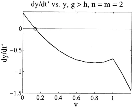
In Figures 12 - 14,

Y

is plotted as a function of y for g = 0, g = h, and g > h. The series of graphs shows how the unstable thermal mode solution and the stable haline mode solution come closer together as g increases and eventually disappear altogether.

(32)

dy/dt'vs. y, g = h, n = m = 2

0

0.2

0.4

0.6

0.8

1 y

Figure 12: Plot of y vs. y exhibiting all three equilibrium solutions.

dy/dt'vs. y,

g =

0,

n = m = 2

0.4

0.2

0 -0.2

C0

0.2

0.4

0.6

0.8

1 y

Figure 13: Plot of

y

vs. y at g = h, where the stable haline mode solution and unstable thermal mode solution merge.

0.4 0.2 F

0 -0.2-

0.4

-

A-\L7

(33)

dy/dt'vs. y,g>h,n=m=2

0.2

0.4

0.6

0.8 y

Figure 14: Plot of y vs. y for g > h. Only the stable thermal present. The value of g used corresponds to v = 5 x

mode solution is 10-"s-1.

0 -0.51

-1

-1.50

C

1

(34)

6. Conclusions

In this model, as the mixing due to surface wind stress increases, the perturbation necessary to shift the system from the stable thermal equilibrium to the stable haline equilibrium increases. Once a critical value is reached, the haline mode equilibrium solution is suppressed entirely. Therefore, if this idealized model accurately represents the real climate, and the circulation due to wind stress were strong enough, the

thermohaline circulation could not switch to another equilibrium state in which sinking occurred at the tropics. These results are consistent with the findings of Shaffer and Olsen (2001) and Longworth et al (2004) using different models. Furthermore, this model has the advantage of an analytical solution, so that an expression can be found for

the critical strength of wind forcing, v D = S '' to first order, necessary to fully EDaC2kT

suppress the haline mode equilibrium. While these results shed light on the way in which wind forcing may affect the circulation patterns in the North Atlantic, it is important to keep in mind that the actual circulation is much more complex than this model, and many factors that could not be considered in such a model may have important effects. In addition, future work might extend this model to include a parameterization that couples the wind-driven mixing term to other variables in order to study any feedbacks that may occur.

(35)

References

Krasovskiy, Y. P., and P. H. Stone (1998), Destabilization of the thermohaline circulation by atmospheric transports: an analytic solution, Journal of Climate, 11,

1803-1811.

Longworth, H., J. Marotzke and T. F. Stocker (2004), Ocean gyres and abrupt change in thermohaline circulation and climate, Journal of Climate (manuscript submitted to journal of climate).

Marotzke, J. (1996), Analysis of thermohaline feedbacks, Decadal Climate Variability:

Dynamics and Predictability, D. Anderson and J. Willebrand, Eds.,

Springer-Verlag, 333-378.

Marotzke, J., and P. H. Stone (1995), Atmospheric transports, the thermohaline

circulation, and flux adjustments in a simple coupled model, Journal of Physical

Oceanography, 25, 1350-1364.

Nakamura, M., P. H. Stone, and J. Marotzke (1994), Destabilization of the thermohaline circulation by atmospheric eddy transports, Journal of Climate, 7, 1870-1882. Shaffer, G., and S. M. Olsen (2001), Sensitivity of the thermohaline circulation and

climate to ocean exchanges in a simple coupled model, Climate Dynamics, 17, 433-444.

Stommel, H. (1961), Thermohaline Convection with Two Stable Regimes of Flow,

Tellus, 13, 224-230.

Stone, P. H. (2004), Climate predictions: the limits of ocean models, in The state of the

Planet: Frontiers and Challenges in Geophysics, Geophysical Monograph, vol.

150, edited by R. S. J. Sparks and C. J. Hawkesworth, pp. 259-267, AGU, Washington, D. C.