Fluid demixing kinetics on spherical geometry: power spectrum and Minkowski functional analysis

(1)

Here plots for all DDFT calculations can be found. (a)

2

4

6

8

10

12

14 l

0

10

20

30

40

50 C

l

10

0

10

1

10

2

10

3

10

4

10

5

t

∗ (b)

1

2

3

4

5

6 l

0

10

20

30

40

50 C

l

10

0

10

1

10

2

10

3

10

4

10

5

t

∗ (c)

2

4

6

8

10

12

14 l

0

10

20

30

40

50 C

l

10

0

10

1

10

2

10

3

10

4

10

5

t

∗ (d)

1

2

3

4

5

6 l

0

50

100

150

200 C

l

10

0

10

1

10

2

10

3

10

4

10

5

t

∗ (e)

2

4

6

8

10

12

14 l

0

20

40

60

80

100

120

140

160

180 C

l

10

0

10

1

10

2

10

3

10

4

10

5

t

∗ (f )

1

2

3

4

5

6 l

0

50

100

150

200

250

300 C

l

10

0

10

1

10

2

10

3

10

4

10

5

t

∗ (g)

2

4

6

8

10

12

14 l

0

50

100

150

200

250

300 C

l

10

0

10

1

10

2

10

3

10

4

10

5

t

∗ (h)

1

2

3

4

5

6 l

0

50

100

150

200

250

300

350

400 C

l

10

0

10

1

10

2

10

3

10

4

10

5

t

∗ (i)

2

4

6

8

10

12

14 l

0

100

200

300

400

500 C

l

10

0

10

1

10

2

10

3

10

4

10

5

t

∗ (j)

1

2

3

4

5

6 l

0

100

200

300

400

500 C

l

10

0

10

1

10

2

10

3

10

4

10

5

t

∗

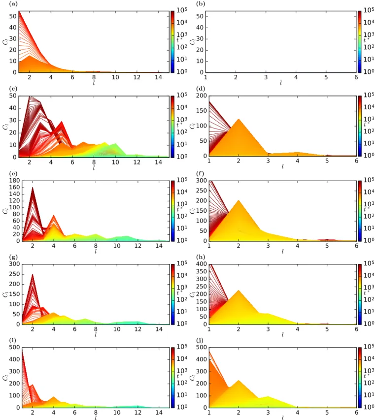
Figure 1. Angular power spectral density. Time t∗is color coded. First column: Large sphere R = 10R11, second column:

(2)

(a) 0.0 0.2 0.4 0.6 0.8 1.0

ρ

th

/ρ

th, 100 0 2 4 6 8 10 12

M

0 (1 00 0 Api x ) 100 101 102 103 104 105

t

∗ (b) 0.0 0.2 0.4 0.6 0.8 1.0

ρ

th

/ρ

th, 100 0 1 2 3 4 5 6

M

1 (1 00 0 q Api x ) 100 101 102 103 104 105

t

∗ (c) 0.0 0.2 0.4 0.6 0.8 1.0 ρth/ρth,100 20 10 0 10 20 30 40 M2 100 101 102 103 104 105

t

∗ (d) 0.0 0.2 0.4 0.6 0.8 1.0

ρ

th

/ρ

th, 100 0 2 4 6 8 10 12

M

0 (1 00 0 Api x ) 100 101 102 103 104 105

t

∗ (e) 0.0 0.2 0.4 0.6 0.8 1.0

ρ

th

/ρ

th, 100 0 1 2 3 4 5 6

M

1 (1 00 0 q Api x ) 100 101 102 103 104 105

t

∗ (f ) 0.0 0.2 0.4 0.6 0.8 1.0 ρth/ρth,100 20 10 0 10 20 30 40 M2 100 101 102 103 104 105

t

∗ (g) 0.0 0.2 0.4 0.6 0.8 1.0

ρ

th

/ρ

th, 100 0 2 4 6 8 10 12

M

0 (1 00 0 Api x ) 100 101 102 103 104 105

t

∗ (h) 0.0 0.2 0.4 0.6 0.8 1.0

ρ

th

/ρ

th, 100 0 1 2 3 4 5 6

M

1 (1 00 0 q Api x ) 100 101 102 103 104 105

t

∗ (i) 0.0 0.2 0.4 0.6 0.8 1.0 ρth/ρth,100 20 10 0 10 20 30 40 M2 100 101 102 103 104 105

t

∗ (j) 0.0 0.2 0.4 0.6 0.8 1.0

ρ

th

/ρ

th, 100 0 2 4 6 8 10 12

M

0 (1 00 0 Api x ) 100 101 102 103 104 105

t

∗ (k) 0.0 0.2 0.4 0.6 0.8 1.0

ρ

th

/ρ

th, 100 0 1 2 3 4 5 6

M

1 (1 00 0 q Api x ) 100 101 102 103 104 105

t

∗ (l) 0.0 0.2 0.4 0.6 0.8 1.0 ρth/ρth,100 20 10 0 10 20 30 40 M2 100 101 102 103 104 105

t

∗ (m) 0.0 0.2 0.4 0.6 0.8 1.0

ρ

th

/ρ

th, 100 0 2 4 6 8 10 12

M

0 (1 00 0 Api x ) 100 101 102 103 104 105

t

∗ (n) 0.0 0.2 0.4 0.6 0.8 1.0

ρ

th

/ρ

th, 100 0 1 2 3 4 5 6

M

1 (1 00 0 q Api x ) 100 101 102 103 104 105

t

∗ (o) 0.0 0.2 0.4 0.6 0.8 1.0 ρth/ρth,100 20 10 0 10 20 30 40 M2 100 101 102 103 104 105

t

∗

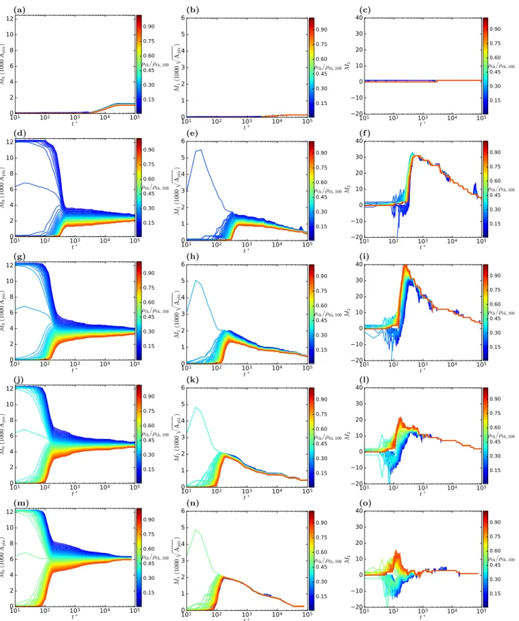
Figure 2. Minkowski functionals dependence on the threshold density ρth/ρth,100 for the large sphere R = 10R11. Time t∗is

(3)

(a) 0.0 0.2 0.4 0.6 0.8 1.0

ρ

th

/ρ

th, 100 0 2 4 6 8 10 12

M

0 (1 00 0 Api x ) 100 101 102 103 104 105

t

∗ (b) 0.0 0.2 0.4 0.6 0.8 1.0 ρth/ρth,100 0 20 40 60 80 100 M1 (1 00 q Api x ) 100 101 102 103 104 105

t

∗ (c) 0.0 0.2 0.4 0.6 0.8 1.0

ρ

th

/ρ

th, 100 4 2 0 2 4 M2 100 101 102 103 104 105

t

∗ (d) 0.0 0.2 0.4 0.6 0.8 1.0

ρ

th

/ρ

th, 100 0 2 4 6 8 10 12

M

0 (1 00 0 Api x ) 100 101 102 103 104 105

t

∗ (e) 0.0 0.2 0.4 0.6 0.8 1.0 ρth/ρth,100 0 20 40 60 80 100 M1 (1 00 q A pi x ) 100 101 102 103 104 105

t

∗ (f ) 0.0 0.2 0.4 0.6 0.8 1.0

ρ

th

/ρ

th, 100 4 2 0 2 4 M2 100 101 102 103 104 105

t

∗ (g) 0.0 0.2 0.4 0.6 0.8 1.0

ρ

th

/ρ

th, 100 0 2 4 6 8 10 12

M

0 (1 00 0 Api x ) 100 101 102 103 104 105

t

∗ (h) 0.0 0.2 0.4 0.6 0.8 1.0 ρth/ρth,100 0 20 40 60 80 100 M1 (1 00 q Api x ) 100 101 102 103 104 105

t

∗ (i) 0.0 0.2 0.4 0.6 0.8 1.0

ρ

th

/ρ

th, 100 4 2 0 2 4 M2 100 101 102 103 104 105

t

∗ (j) 0.0 0.2 0.4 0.6 0.8 1.0

ρ

th

/ρ

th, 100 0 2 4 6 8 10 12

M

0 (1 00 0 Api x ) 100 101 102 103 104 105

t

∗ (k) 0.0 0.2 0.4 0.6 0.8 1.0 ρth/ρth,100 0 20 40 60 80 100 M1 (1 00 q A pi x ) 100 101 102 103 104 105

t

∗ (l) 0.0 0.2 0.4 0.6 0.8 1.0

ρ

th

/ρ

th, 100 4 2 0 2 4 M2 100 101 102 103 104 105

t

∗ (m) 0.0 0.2 0.4 0.6 0.8 1.0

ρ

th

/ρ

th, 100 0 2 4 6 8 10 12

M

0 (1 00 0 Api x ) 100 101 102 103 104 105

t

∗ (n) 0.0 0.2 0.4 0.6 0.8 1.0 ρth/ρth,100 0 20 40 60 80 100 M1 (1 00 q Api x ) 100 101 102 103 104 105

t

∗ (o) 0.0 0.2 0.4 0.6 0.8 1.0

ρ

th

/ρ

th, 100 4 2 0 2 4 M2 100 101 102 103 104 105

t

∗

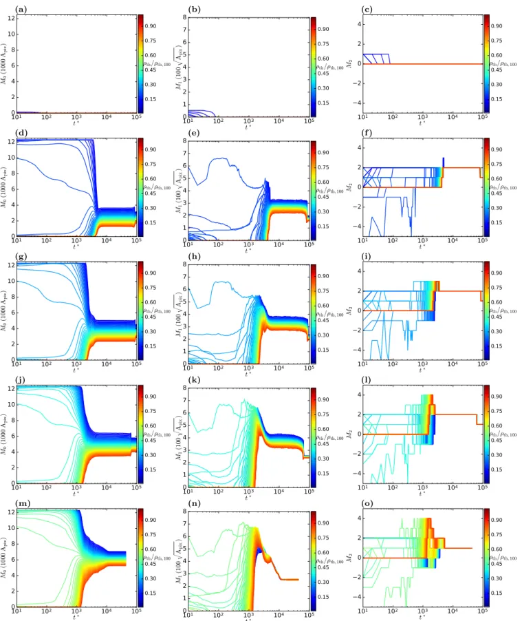
Figure 3. Minkowski functionals dependence on the threshold density ρth/ρth,100for the small sphere R = 2.5R11. Time t∗is

color coded. First column: Area functional M0, second column: perimeter functional M1, third column: euler functional M2.

(4)

For early times of spinodal decomposition the time dependent functionals (Fig. 4 and Fig. 5) vary for different threshold density values. However, for later times the functionals become constant functions of ρth due to the

emergence of well defined demixed domains. The functionals have their greatest variations at relative threshold values in the vicinity of the mixture parameter ρth/ρth,100' x. The variation of the functionals at ρth/ρth,100 ' x

decreases as time evolves due to the decrease of interfaces in the stage of domain coalescence. After the crossover time t∗c between the spinodal decomposition and domain growth phase the functionals become constant functions.

The area functionals M0 for large times approach the constant value of the complete surface V0 weighted with the

mixing parameter x: V (t → ∞) = V0x. Correspondingly the perimeter functionals M1converge towards the value of

the boundary length of the corresponding spherical cap. The Euler functional M2 converges to the constant number

of already demixed domains. For the extreme values of T on can observe peaks in M1 and M2 that originate from

an artefact of the numerical implementation: the calculation of functional derivatives is done via convolutions of the spherical harmonical decomposition leading to overshoots at sharp edges of density variations at pixel boundaries. Since the analysis in the main paper only depends on intermediate values of ρth this does not pose a problem.

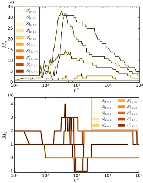
The number of domains can readily be obtained as the value of the Euler functional M2 (Fig. 8 ). It counts the

number of connected domains and substracts the number of holes in the domains. Since for non-extreme threshold values (near the boundaries, e.g, ρth/ρth,100 = 0 and ρth/ρth,100 = 1) there are no holes in the domains, and the

(5)

(a) 101 ₁₀2 103 104 ₁₀5 t∗ 0 2 4 6 8 10 12 M0 (1 00 0 Api x ) 0.15 0.30 0.45 0.60 0.75 0.90 ρth/ρth, 100 (b) 101 ₁₀2 ₁₀3 ₁₀4 ₁₀5 t∗ 0 1 2 3 4 5 6 M1 (1 00 0 q Api x ) 0.15 0.30 0.45 0.60 0.75 0.90 ρth/ρth, 100 (c) 101 ₁₀2 ₁₀3 ₁₀4 ₁₀5 t∗ 20 10 0 10 20 30 40 M2 0.15 0.30 0.45 0.60 0.75 0.90 ρth/ρth,100 (d) 101 102 103 104 105 t∗ 0 2 4 6 8 10 12 M0 (1 00 0 Api x ) 0.15 0.30 0.45 0.60 0.75 0.90 ρth/ρth, 100 (e) 101 ₁₀2 ₁₀3 ₁₀4 ₁₀5 t∗ 0 1 2 3 4 5 6 M1 (1 00 0 q A pi x ) 0.15 0.30 0.45 0.60 0.75 0.90 ρth/ρth, 100 (f ) 101 ₁₀2 ₁₀3 ₁₀4 ₁₀5 t∗ 20 10 0 10 20 30 40 M2 0.15 0.30 0.45 0.60 0.75 0.90 ρth/ρth,100 (g) 101 ₁₀2 ₁₀3 ₁₀4 ₁₀5 t∗ 0 2 4 6 8 10 12 M0 (1 00 0 Api x ) 0.15 0.30 0.45 0.60 0.75 0.90 ρth/ρth, 100 (h) 101 ₁₀2 ₁₀3 ₁₀4 ₁₀5 t∗ 0 1 2 3 4 5 6 M1 (1 00 0 q Api x ) 0.15 0.30 0.45 0.60 0.75 0.90 ρth/ρth, 100 (i) 101 ₁₀2 ₁₀3 ₁₀4 ₁₀5 t∗ 20 10 0 10 20 30 40 M2 0.15 0.30 0.45 0.60 0.75 0.90 ρth/ρth,100 (j) 101 102 103 104 105 t∗ 0 2 4 6 8 10 12 M0 (1 00 0 Api x ) 0.15 0.30 0.45 0.60 0.75 0.90 ρth/ρth, 100 (k) 101 ₁₀2 ₁₀3 ₁₀4 ₁₀5 t∗ 0 1 2 3 4 5 6 M1 (1 00 0 q Api x ) 0.15 0.30 0.45 0.60 0.75 0.90 ρth/ρth, 100 (l) 101 ₁₀2 ₁₀3 ₁₀4 ₁₀5 t∗ 20 10 0 10 20 30 40 M2 0.15 0.30 0.45 0.60 0.75 0.90 ρth/ρth,100 (m) 101 102 103 104 105 t∗ 0 2 4 6 8 10 12 M0 (1 00 0 Api x ) 0.15 0.30 0.45 0.60 0.75 0.90 ρth/ρth, 100 (n) 101 ₁₀2 ₁₀3 ₁₀4 ₁₀5 t∗ 0 1 2 3 4 5 6 M1 (1 00 0 q A pi x ) 0.15 0.30 0.45 0.60 0.75 0.90 ρth/ρth, 100 (o) 101 ₁₀2 ₁₀3 ₁₀4 ₁₀5 t∗ 20 10 0 10 20 30 40 M2 0.15 0.30 0.45 0.60 0.75 0.90 ρth/ρth,100

Figure 4. Minkowski functionals, dependence on time t∗, for the large sphere R = 10R11. Threshold values ρth/ρth,100 are

(6)

(a) 101 ₁₀2 103 104 ₁₀5 t∗ 0 2 4 6 8 10 12 M0 (1 00 0 Api x ) 0.15 0.30 0.45 0.60 0.75 0.90 ρth/ρth, 100 (b) 101 ₁₀2 ₁₀3 ₁₀4 ₁₀5 t∗ 0 1 2 3 4 5 6 7 8 M1 (1 00 q A pi x ) 0.15 0.30 0.45 0.60 0.75 0.90 ρth/ρth, 100 (c) 101 ₁₀2 ₁₀3 ₁₀4 ₁₀5 t∗ 4 2 0 2 4 M2 0.15 0.30 0.45 0.60 0.75 0.90 ρth/ρth, 100 (d) 101 102 103 104 105 t∗ 0 2 4 6 8 10 12 M0 (1 00 0 Api x ) 0.15 0.30 0.45 0.60 0.75 0.90 ρth/ρth, 100 (e) 101 ₁₀2 ₁₀3 ₁₀4 ₁₀5 t∗ 0 1 2 3 4 5 6 7 8 M1 (1 00 q Api x ) 0.15 0.30 0.45 0.60 0.75 0.90 ρth/ρth, 100 (f ) 101 102 103 104 105 t∗ 4 2 0 2 4 M2 0.15 0.30 0.45 0.60 0.75 0.90 ρth/ρth, 100 (g) 101 ₁₀2 ₁₀3 ₁₀4 ₁₀5 t∗ 0 2 4 6 8 10 12 M0 (1 00 0 Api x ) 0.15 0.30 0.45 0.60 0.75 0.90 ρth/ρth, 100 (h) 101 ₁₀2 ₁₀3 ₁₀4 ₁₀5 t∗ 0 1 2 3 4 5 6 7 8 M1 (1 00 q Api x ) 0.15 0.30 0.45 0.60 0.75 0.90 ρth/ρth, 100 (i) 101 102 103 104 105 t∗ 4 2 0 2 4 M2 0.15 0.30 0.45 0.60 0.75 0.90 ρth/ρth, 100 (j) 101 102 103 104 105 t∗ 0 2 4 6 8 10 12 M0 (1 00 0 Api x ) 0.15 0.30 0.45 0.60 0.75 0.90 ρth/ρth, 100 (k) 101 ₁₀2 ₁₀3 ₁₀4 ₁₀5 t∗ 0 1 2 3 4 5 6 7 8 M1 (1 00 q Api x ) 0.15 0.30 0.45 0.60 0.75 0.90 ρth/ρth, 100 (l) 101 102 103 104 105 t∗ 4 2 0 2 4 M2 0.15 0.30 0.45 0.60 0.75 0.90 ρth/ρth, 100 (m) 101 102 103 104 105 t∗ 0 2 4 6 8 10 12 M0 (1 00 0 Api x ) 0.15 0.30 0.45 0.60 0.75 0.90 ρth/ρth, 100 (n) 101 ₁₀2 ₁₀3 ₁₀4 ₁₀5 t∗ 0 1 2 3 4 5 6 7 8 M1 (1 00 q Api x ) 0.15 0.30 0.45 0.60 0.75 0.90 ρth/ρth, 100 (o) 101 102 103 104 105 t∗ 4 2 0 2 4 M2 0.15 0.30 0.45 0.60 0.75 0.90 ρth/ρth, 100

Figure 5. Minkowski functionals, dependence on time t∗, for the small sphere R = 2.5R11. Threshold values ρth/ρth,100 are

(7)

101 ₁₀2 ₁₀3 ₁₀4 ₁₀5

t

∗ 10-2 10-1 100 101 102 103

(2

l

+

1)

·

C

l,m

ax

S2 10,0.1 S2 10,0.2 S2 10,0.3 S2₁₀_,₀_.₄ S2 10,0.5 S2 2.5,0.1 S2 2.5,0.2 S2 2.5,0.3 S2₂_.₅_,₀_.₄ S2 2.5,0.5

Figure 6. Power spectrum analysis: Power (2l + 1)Cl,max of the maximum of the angular power spectrum Cl,max =

max1<l<N(Cl). 101 ₁₀2 ₁₀3 ₁₀4 ₁₀5

t

∗ 101 102 103

M

1

(

A

pi x

)

S2 10, 0. 1 S2 10, 0. 2 S2 10, 0. 3 S2 10, 0. 4 S2 10, 0. 5 S2 2. 5, 0. 1 S2 2. 5, 0. 2 S2 2. 5, 0. 3 S2 2. 5, 0. 4 S2 2. 5, 0. 5

Figure 7. Circumference Minkowski functionals M1 for threshold values T /T100' x. Exact threshold values are ρth/ρth,100∈

(8)

(a) 101 ₁₀2 ₁₀3 ₁₀4 ₁₀5

t

∗ 0 5 10 15 20 25 30 35

M

2 S2 10, 0. 1 S2 10, 0. 2 S2 10, 0. 3 S2 10, 0. 4 S2 10, 0. 5 S2 2. 5, 0. 1 S2 2. 5, 0. 2 S2 2. 5, 0. 3 S2 2. 5, 0. 4 S2 2. 5, 0. 5 (b) 101 ₁₀2 ₁₀3 ₁₀4 ₁₀5

t

∗ −1 0 1 2 3 4

M

2 S2 10, 0. 1 S2 10, 0. 2 S2 10, 0. 3 S2 10, 0. 4 S2 10, 0. 5 S2 2. 5, 0. 1 S2 2. 5, 0. 2 S2 2. 5, 0. 3 S2 2. 5, 0. 4 S2 2. 5, 0. 5

Figure 8. Euler characteristic Minkowski functional M2 for threshold values T /T100 ' x. Exact threshold values are