Fluid demixing kinetics on spherical geometry: power spectrum and Minkowski functional analysis

PAPER • OPEN ACCESS

Fluid demixing kinetics on spherical geometry: power spectrum and

Minkowski functional analysis

To cite this article: A Böbel et al 2019 New J. Phys. 21 013031

View the article online for updates and enhancements.

PAPER

Fluid demixing kinetics on spherical geometry: power spectrum and

Minkowski functional analysis

A Böbel1

, M C Bott2

, H Modest1

, J M Brader2

and C Räth1

1 _{Institut für Materialphysik im Weltraum, Deutsches Zentrum für Luft- und Raumfahrt(DLR), Münchener Str. 20, D-82234, Weßling,}

Germany

2 _{Soft Matter Theory, University of Fribourg, Switzerland}

E-mail:[email protected]

Keywords: morphological data analysis, demixing, curved space, spinodal decomposition Supplementary material for this article is availableonline

Abstract

Dynamic density functional theory calculations of

fluid–fluid demixing on spherical geometries are

characterized via their angular power spectrum as well as via the Minkowski functionals

(MFs) of their

binarized

fluid density fields. MFs form a complete set of additive, motion invariant and continuous

morphological measures sensitive to nonlinear

(spatial) correlations. The temporal evolution of the

fluid density fields is analyzed for different sphere sizes and mixing compositions. The demixing

process in the stages of early spinodal decomposition and consecutive domain growth can be

characterized by both methods and a power-law domain growth

L t

( )

µ

t is evidenced for the MF

measures. The average domain size obtained by the structure factor only responds to the late stage

domain growth of the demixing process. MFs provide refined insights into the demixing process: they

allow the detection of distinct stages in the early spinodal decomposition, provide a precise measure of

the relative species composition of the mixture and, most importantly: after a proper rescaling, they

allow the detection of a universal demixing behavior for a wide range of mixture fractions and for

different sphere sizes.

1. Introduction

If a binaryfluid mixture is in the immiscible state it will start to dynamically demix in order to reach the thermodynamically stable state of two coexisting phases. This phase separation can be split in two consecutive regimes[1–3]: the spinodal decomposition in the early stage, followed by the domain growth stage. During spinodal decompositionfluid density fluctuations increase exponentially and neighboring particles agglomerate to form disjoint domains. In the domain growth stage the size of these initial domains increases further and they start to coalesce with neighboring domains in order to reduce the energy costs of the interface areas. As the domain morphology is preserved, this domain growth is self-similar in time. The self-similarity implies a time-dependent characteristic length of the mean domain size that can be described by a power-law

growthL t( )µta.

When the system is spatially confined, the phase separation kinetics are less well understood. Spatial confinement can be imposed by obstacles and external fields [4,5]. Another form of spatial confinement can be achieved via the geometry of space itself[6]. Recently, the study of statistical physics processes on curved surfaces, in particular on the sphere, has attracted growing interest and showed the richness of physical phenomena that are influenced by their embedding on non-flat geometries. The crystallization of a colloidal suspension on a sphere was explained via a icosahedrically symmetric order parameter that revealed the long-range order of the crystal on the curved surface[7]. The projection of inhomogeneous crystals onto homogeneous ones on curved surfaces enabled the prediction of defect distributions[8]. Also, unusual emergent structures due to advection were demonstrated on a spherical geometry[9].

OPEN ACCESS

RECEIVED 4 October 2018 REVISED 30 November 2018 ACCEPTED FOR PUBLICATION 17 December 2018 PUBLISHED 30 January 2019

Original content from this work may be used under the terms of theCreative Commons Attribution 3.0 licence.

Any further distribution of this work must maintain attribution to the author(s) and the title of the work, journal citation and DOI.

Common methods for the characterization of demixing dynamics are based on linear measures: the mean domain size is measured via thefirst zero crossing of the radial correlation function or equivalently via the first maximum of the power spectral structure factor[10–12]. However, this method is computationally expensive [13]. Another drawback lies in the linearity of the method. The mean domain size is not a sufficient descriptor of the domain morphology[3,14,15]. Thus, it is beneficial to extend the description of the demixing system to morphological measures, which are sensitive to higher order correlations.

Morphological measures that capture the complete nonlinear structural information of a system are the Minkowski functionals(MFs) [16]. They became a prominent tool for morphological data analysis since they form a complete family of structural descriptors sensitive to nonlinear properties. MFs are well suited for the investigation of demixing processes[3,14,15] and can readily be applied on spherical geometry [17–19]. In two-dimensionalflat and curved spaces the MFs are easily interpretable measures connected to concepts as area, perimeter and the Euler characteristic. The Euler characteristic is a measure for the connectivity of a spatial structure.

In this work we aim to systematically study the properties of dynamic density functional theory calculations (DDFT) of fluid demixing on a spherical geometry with both linear and nonlinear measures. The DDFT calculations were already utilized as the basis for the studies in[6] and are reused here as a convenient starting point for thefirst ever MF analysis of fluid–fluid demixing on spherical geometries. Initially we apply the conventional linear method known in theflat space case to the spherical data: we calculate the angular power spectral density andfit it to a general structure factor function in order to calculate the average domain size L. These results are then compared with the MF measures.

This paper is structured as follows: in section2we explain the methods and results for the calculation of the phase separation dynamics on the spherical body. Section3describes the method of the structure factor calculation based on the angular power spectral density and the implementation of the MF calculation. The results of power spectral density and MF analysis for DDFT calculations with different sphere sizes and mixture parameters are presented in section4. Finally, in section5results are discussed and conclusions drawn.

2. Dynamic density functional theory calculations

This section is intended to give a brief overview of the methods and results found about phase separation on a large spherical particle[6]. The data for the evolution of the density distribution during spinodal decomposition forms the basis for the MF analysis discussed in this manuscript.

In order to avoid any confusion with terminology, we will henceforth refer to the large particle as the ‘meso-particle’ and the smaller, mobile particles constituting the fluid on its surface as the ‘surface particles’.

2.1. The Gaussian core model(GCM)

To represent the surface particles, we consider a model binary mixture, thus two particle species, in which the particles interact via the soft repulsive pair potential



bv rij( )=b ijexp{-r2 Rij2}. ( )1

Here the non-negative parametersòij, Rijand b =(k TB )-1determine the strength and range, respectively, of the interaction between species i and j. The GCM was introduced by Stillinger[20] to study phase separation in binary mixtures and has since been studied intensively, both in bulk and at interfaces[21]. The model has the advantage that a simple mean-field approximation to the free energy provides good agreement with computer simulation data[22] and is therefore straight forward to incorporate in a density functional theory.

2.2. Mean-field free energy functional

To describe the collective behavior of the surface particles we use an approximation to the two-dimensional Helmholtz free energy functional



ò

ò ò

å

å

where thefirst and second terms provide the ideal and excess (over ideal, describing the particle interactions) contributions, respectively. The subscripts i and j are species labels and the notation[{ ( )}]r_i r indicates a functional dependence on the one-body density profiles of all species. We set the (physically irrelevant) thermal wavelengthλ equal to unity. For a binary mixture the species indicies are restricted to the values i, j=1, 2.

In bulk, the number density of species i isr = N V_i i , where V is the area in the 2d case and Nithe number of

particles of species i. The total density is of the surface particlesρ=ρ1+ρ2.

It is convenient to introduce a concentration variable, the mixture parameter x=N2/N, with the total

number of particles N. This enables the species labeled densities to be expressed asρ1=(1−x)ρ and ρ2=xρ. In

these variables the bulk free energy per particle consists of a sum of two terms, fºF N=f_id +f_ex. The ideal part is given by

bf_id =ln( )r - +1 (1-x)ln 1( -x)+xln( )x , ( )3 and the reduced bulk excess free energy per particle can be written as

b r r r r r r r = ( ˆ + ˆ + ˆ ) ( ) f 1 v v v 2 2 . 4 ex 1 1 11 1 2 12 2 2 22

wherevˆij =*ijRij2pand *ij =bij. In[6] the parametersR11=R22=R12=1, *11=*22= 2and *12= 1.035*11

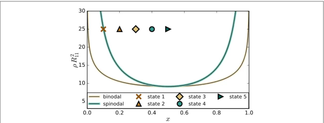
where chosen and the phase diagram for an infinite planar system has been calculated. This phase diagram is shown infigure1and indicates thefive states that will be analyzed in this study for a large R=10R11, respectively

a small R=2.5R11sphere. Even though the meso-sphere represents afinite size system the phase diagram for

the bulk system offers a useful guide. When the total densityρ becomes sufficiently large the GCM demixes. 2.3. Dynamical density functional theory and numerical implementation

To study phase separation on the surface of a meso-particle we will focus on the dynamics of the one-body density of the surface particles. This can be obtained using DDFT[23,24]. Within this approach the time evolution of the density of species i is given by a

 g r r d r dr ¶ ¶ = ¶ ¶ ¶ ¶ - ⎡ ⎣ ⎢ ⎤ ⎦ ⎥ ( ) · ( ) [{ ( )}] ( ) ( ) t t t t t r r r r r r , , , , . 5 i i i i 1

Hereγ is the mobility and it is related to the diffusion coefficients D as γ=βD. The DDFT equation of motion (5) is a generalized diffusion equation. The one-body density is driven by gradients in the local chemical potential which arise from the particle interaction described by the functional for the free energy(2). If we insert the functional of the ideal gas, we recover the well known diffusion equation for a non interacting gas.

To solve the DDFT equation of motion(5) on the surface of a meso-sphere we chose to parametrize the sphere using the spherical polar anglesθ and f. With this approach we have an accurate finite-difference scheme for calculating the gradient and divergence of scalar- and vectorfields. In addition we make use of the

convolution theorem on the unit-sphere[6,25] to efficiently compute the convolution of two scalar fields in the space of spherical harmonic functions. The numerical methods for solving equation(5) on the surface of a sphere are described in more detail in[6].

2.4. DDFT calculation results

For larger meso-sphere radii(R = 10R11) we find standard spinodal decomposition dynamics for an equal

mixture, x=0.5, leading to a ‘half–half’ final state. As the value of x is reduced towards the spinodal, then the Figure 1. Phase diagram for the planar system as a reference point. Binodal and spinodal curves, as well as the states analyzed in this study are indicated. The states arexÎ {0.1, 0.2, 0.3, 0.4, 0.5 for r} R₁₁2=25_{. Parameters areR =R =R =1}

11 22 12 , *11=*22= 1,

* *

phase separation dynamics are given by the Ostwald ripening scenario[26], where islands of the minority phase form, which then slowly merge together(see figure2). For the phase separation on the smaller meso-particle (R = 2.5R11) finite-size effects become more important. In contrast to the behavior on the larger meso-sphere,

the density evolves here in most cases into a‘band’ state, where two islands with species 1 form, separated by a band of species 2 particles. This state is stable over a long time. The smaller we chose the mixture parameter x the longer the metastable band state lives. This enhanced stability of the band structure can be attributed to the fact that the distance between the interfaces increases as the surface coverage of the minority phase is reduced by reducing x. In the following analyses we only consider one of the species and call its densityfield

* *

r₂(r,t )ºr(r,t ). Since their contributions are mirror images their information content is redundant. t*is the dimensionless time given by * =t tD R₁₁2_{, where D is the bare diffusion coefficient.}

Movies for all DDFT calculations are provided in the supplemental material available online atstacks.iop. org/NJP/21/013031/mmedia.

2.5. Equal area pixelisation

Using the python library healpy[27] for HEALPix the spherical coordinate grid (181×92=16652 pixel) was interpolated on a equal area pixel grid with Npix=12 288 pixel in order to apply the MF analysis

straightforwardly. The HEALPix pixelisation scheme is a partition of a spherical surface into exactly equal area quadrilateral pixels of varying shape[28] but uniform area Apix. The pixel size depends on the HEALPix

resolution parameter of the grid equal toNside=1, 2, 4, 8,¼corresponding to a total number of pixels of

= ´ = ¼

Npix 12 Nside2 12, 48, 192, 768, In this work we use a resolution parameter of Nside=32, since this is

the closest match to the raw data in the spherical coordinate grid. In further studies much higher resolutions can be obtained. Infigure2the pixelization of the densityfieldsr(r,t*)is shown for both sphere sizes during the evolution of time t*.

Figure 2. Mollweide projection of equal area pixelisation for the DDFT calculation data for x=0.3. Left column: (a), (c), (e), (g) Evolution of the particle densityr (₂r,t*)of species two for the large sphere R=10R11. Right column:(b), (d), (f), (h) Evolution of

3. Spatial statistics

3.1. Angular power spectral density

Any scalar functionr( )n on a spherical geometry, wheren ,(q f)is a direction on the sphere, can be

decomposed into its spherical harmonics representation. The spherical harmonics Ylmform an orthonormal

base on the unit sphere. They are given by:

p q = + -+ f ( )! ( )! ( ( )) ( ) Y l l m l m P 2 1 4 cos e . 6 lm lm im

With indiceslÎ0and-lml. Plmare the Legendre polynomials. l is the multipole. The average solid

angleΩ corresponding to a specific l is Ω=4π/2l. Considering the division of the sphere in 2l equal slices, the widest part of these slices corresponds to an angleγ=π/l. This translates into a length scale L=R·π/l, with the sphere radius R.

Thenr( )n can be expanded as:

 

å å

with harmonic coefficients almgiven by the projection

*

ò

= W ( ) ( ) ( )

alm d n Ylmn . 8

*

◦ denotes the complex conjugate of◦. The power spectrum Clof the scalarfield ρ(n) can be defined as the

variance of the harmonic coefficientsáa alm l m*_{¢ ¢}ñ =d dll¢ mm¢Clwith



å

The Clare called the angular power spectral density. Since for any l there exist 2l+1 modes of m the total power

for the multipole l is given by(2l+1) ·Cl.

In the following we analyze the positionlmaxand value Cl,maxof the maximum of the power spectral density.

lmaxis a measure for the length scale of the most dominant pattern. This quantity is the standard metric to

characterize the domain growth of demixing processes[2,3,12,13,29]. Here we also introduce the power Cl,max as a measure for the domain growth. Cl,maxis a measure for the dominance of the most predominant pattern(in terms of spherical harmonics) of the function on the sphere.

The position of the maximum is determined, using the standard procedure, viafitting the off-critical fitting functionS l t(, )µ( ·l LPS( )t 2p)2 [2+( ·l LPS( )t 2p) ]6 [30] and the average domain size LPSis identified

as pR lmax.

3.2. Minkowski functionals

Since the early 20th century[16] MFs have been known in integral geometry [31,32] and became a prominent tool for morphological data analysis[33]. They are able to characterize the geometry and shape of structural data as well as their topology and connectedness. MFs are sensitive to any n-point correlation function and thus can provide new insights into physical processes beyond the capability of linear methods, e.g. power spectral density measures.

On the two-dimensional sphere 2_{with radius R in D=2 dimensions the D+1 MFs n Î}

n { }

M , 0, 1, 2

for a setKÍ2_{are the area M}

0, the perimeter M1and the Euler characteristic M2. They are defined as:

ò

ò

ò

Here,κ (r) is the local Gaussian curvature.

MFs are motion invariant, additive and conditionally continuous. They form a complete family of

morphological measures. Or vice versa: Any motion invariant, conditionally continuous and additive functional is a superposition of the countably many MFs[34]. They are nonlinear measures sensitive to any higher order correlations. They are homogeneous functions of orderD-n:

l =l

n( ) -n n( ) ( )

There is a broad range of applications of MFs, e.g. curvature energy of membranes[35], order parameter in Turing patterns[36], density functional theory for fluids (as hard balls or ellipsoids) [37,38], testing point distributions(find clusters, filaments, underlying point-process) or searching for non-Gaussian signatures in the cosmic microwave background[17–19,39,40].

In order to study the morphology of the smooth, scalar densityfieldsr(r,t*), the MFs of the excursion sets Kthof the equal area pixelization of the simulation data are calculated. Kthis the set of all pixels with density

valuesr(r,t*)that are higher or at least equal to a threshold valueρth:Kth={rÎ2∣ (r r,t*)rth}. These

pixels mark the regionsron 2_{that have a densityr(r,t*)greater or equal to the threshold densityr} th, at the

time t*.

By running over 101 equidistant threshold stepsr_th,k(with Îk {0,¼, 100}) the density fields are binarized into an active and a non-active part. Thefirst threshold stepr_th,0is chosen such that every pixel on 2_{is active.}

The last stepr_th,100is reached when all pixels are excluded and inactive.

For the implementation of the explicit calculation the algorithm proposed in[41] is adapted to compute MFs of pixelized maps: due to the additivity of the MFs the calculation can be performed by the summation of local contributions. Individual pixels are considered to be composed of 4 vertices, 4 edges and their interior area. The total number of active pixels ns, the number of edges neand vertices nvat the interface of active and inactive

pixels is counted. Then the area M0, the integral mean curvature(or perimeter) M1and the Euler characteristic

M2can be calculated as sums:

= = - + = - + M n M n n M n n n 4 2 . 0 s 1 s e 2 s e v

In order to avoid any double counting of edges or vertices the originalfield is built up iteratively by adding active pixels to the initially empty temporaryfield individually. Only if all neighboring pixels have already been built into the temporaryfield the edges and vertices are added to the total sum. The number of arithmetic operations required to compute the MFs scales linearly with the number of active pixels and the total number of pixels of the image.

4. Results

4.1. Power spectral density

The angular power spectral densities obtained for the DDFT calculations on different sphere sizes R and with different mixture parameters x are presented in the supplementary material.

The graphs for the average domain size, measured as the characteristic length scaleLPS=Rp lmax, derived

from the positions of maximal power spectrum amplitudeslmaxare presented infigure3. In these graphs the

initial spinodal decomposition phase of nucleation cannot be observed. LPSis blind for the initial demixing

stage(exponential growth of density fluctuations) where yet no domain growth can be observed. However, in the coalescence stage, an increase of LPSis found that can befitted to a power-law. The power law is better

reproduced in the large sphere graphs, since they allow for more individual domains, more coalescence events Figure 3. Power spectrum analysis: The characteristic length scaleLPS=Rp lmaxis identified via the position of the maximum of the

angular power spectrumlmax=l∣Cl=Cl,max. It is the standard measure for the average domain size. Different sphere radii R and mixture parameters x are color coded. Their values are indicated in the legend by_{R R}2_{/ ,x}

112 .

2_{denotes the two-dimensional sphere. As a guide}

to the eye power-lawfits are presented as green dashes lines. The signal for2.5,0.12 is not shown. It is very small since no demixing

and therefore provide a more constant slope in the log–log plot. The small sphere graphs show plateaus between power law growth. During plateau phases no coalescence of domains happens because of the low number of individual domains on the small sphere. The onset of demixing is much later for the small sphere compared to the large sphere. Also smaller mixture parameters correlate with later times for the onset of demixing. In particular forR=2.5R11and x=0.1 no demixing is observed during the complete DDFT calculation, ending

at * =t 105_{. The domain growth is faster for higher mixture parameters, the exception being x=0.1: here the}

demixing processes starts late but domain growth is fast. 4.2. Minkowski functionals

The dependence of the MFs on the threshold densityρthis presented in the supplementary material.

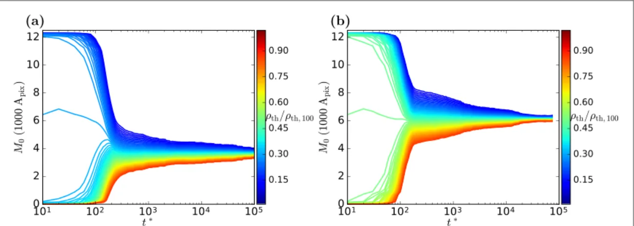
The temporal evolution of the MFs is also presented in the supplementary material. Here two plots are shown representatively:figure4shows the area functional M0for the mixing fractions x=0.3 in panel (a) and

x=0.5 in panel (b). The relative threshold value r r_{th th,100}is color coded. For early times there is a qualitative difference for the regimes r_th r_th,100< xand r_th r_th,100> xfor M0.(AlsoM1(rth)andM2(rth)have a higher

variance in the early time phase during spinodal decomposition. See supplementary material.) The functional at the crossover value r_th r_th,100 xdeviate significantly from the functional values at neighboring threshold values. Any other threshold variations only show small changes in the shape of the curve. In the initial mixture the density is r r_th,100 x, all relative threshold values below x result in almost no active pixels after

binarization, but most pixels are active for higher thresholds. This leads to a sharp transition of the MFs from detecting almost all pixels as active to detecting almost no active pixels at r_th r_th,100 x. Thus it is easy to detect the composition parameter x via the shape of MF curves even only analyzing the initial phase of spinodal decomposition.

After a certain point in time, however, the curves are essentially the same. This point can be identified as the timetc*where the spinodal decomposition transitions from the early nucleation stage to the late stage

coalescence regime. With these curvestc*can easily be determined. In particular using non-morphological

measures like e.g. the correlation function the determination oftc*proves to be more difficult and

computationally expensive[13].

The MF graphs obtained on the sphere are in qualitative agreement with MF calculated for spinodal decomposition inflat two-dimensional geometry [14,15].

4.3. Stages during spinodal decomposition

In the following analysis a specific threshold valuer_this chosen for any DDFT calculation. It is choosen such that the minimal detected number of active pixels is close to 1.(This happens at r r_{th th,100} x.) Then the MFs have a maximal dynamic range. These MF graphs are presented, for the area functional M0, infigure5. In all

functional graphs both, the spinodal decomposition and the subsequent coalescence stage of demixing can be evidenced. During spinodal decomposition the M0area functional follows a power law. In the coalescence stage

it assumes a constant value since the individual domains only grow by merging with neighboring domains. M1

also grows fast during spinodal decomposition. However, during the coalescence stage it drops again, thus providing a means to easily determine the crossover timetc*.(Compare figure6, or consult the supplementary

material.) We obtain *t_c 2´102_{in the case of R=10R}

11and *tc 2´103in the case of R=2.5R11.

A difference in the shape of the graphs for the large and small sphere can be observed: in the large sphere graphs M0has a small, non-vanishing slope before the main growth phase evidences the initial nucleation. This

Figure 4. Area Minkowski functional M0, dependent on the relative threshold density rth rth,100, for large sphereR=10R11.

cannot be observed for the small sphere, where the slope changes rapidly from its zero value in the beginning to a high value in the initial nucleation phase of the spinodal decomposition.(M1shows the same behavior, shown in

the supplementary material.)

In comparison to the power spectrum measure presented infigure3, the MF graphs are not as smooth since they are more sensitive to dynamical changes in the structure of density profiles. This allows the MFs to detect features of the demixing process that is not accessible via power spectrum analysis. The MFs resolve three distinct phases in the early stage of spinodal decomposition with different domain growth rates:(1) prior to the spinodal decomposition,(2) initial spinodal decompostion, (3) main spinodal decomposition. None of these stages can be detected with the standard demixing metric L(t) obtained by the position of the maximum of the power spectral density as can be seen infigure3. When plotting the maximum of the angular power spectrum Cl,maxphases(1) and (2) can also be detected. (Shown in the supplementary material.) Thus, the maximum of the power spectral density is, in contrast to measures obtained by its position, able to detect the densityfluctuation growth characteristic to the spinodal decomposition in the early stage of demixing.

The dynamical range of the MFs depends only on the resolution of the data, since one can alwaysfind a threshold value, such that the minimal number of active pixels is close to one. The upper limit is determined by the number of active pixels after spinodal decomposition which scales with the resolution of the data. The power spectrum analysis does not show such a resolution dependence that provides a higher dynamical range proportional to the resolution. For the power spectral density a higher resolution only provides further modes l. 4.4. Characteristic length scaleL

Since the MFM K are homogeneous function of ordern( ) D-n(equation (11)) one can expect a scaling behavior of the MFs for the scaling length L:

Figure 5. Area Minkowski functional M0for threshold values rth rth,100 x. Exact threshold values are rth rth,100Î [0.134, 0.212,

]

0.316, 0.416, 0.515 4 . Different sphere radii R and mixture parameters x are color coded. Their values are indicated in the legend by

2_{R R/ ,x} 112 .

2_{denotes the two-dimensional sphere.}

Figure 6. Scaling behavior of1 M1µLreveal power law domain growthLµt*aafter spinodal decomposition. Different sphere

radii R and mixture parameters x are color coded. Their values are indicated in the legend by2_{R R/ ,x} 112 .

2_{denotes the two-dimensional}

sphere. As a guide to the eye power-lawfits are presented as green dashes lines. They are shifted in a parallel fashion (by multiplication with the factor 0.8) to enhance visibility.

µ µ - µ - _{( )}

M0 1, M1 L 1, M2 L 2, 12

L can be interpreted as the characteristic size of demixed domains. Note that L can of be defined via different methods, e.g. as thefirst zero crossing of the correlation function or as the first moment of the wavelength distribution[10,11]. These widely used methods are, however, computationally expensive [13]. The scaling behavior of1 M1µLis presented infigure6.(For the plot of1 M2 µLconsult the supplementary material.)

It evidences the power law growth of domain sizeLµt*aduring the coalescence phase after spinodal

decomposition. The transition from spinodal decomposition to coalescence happens at about *t_c 2´102_in

the case ofR=10R11and *tc 2´103in the case ofR=2.5R11.

For the small sphere only few disjoint domains exist and thus only few coalescence events happen where L changes rapidly. The power law can however still be detected via the mean slope in1 M1. For1 M2the few

coalescence events result in non-smooth graphs resulting in poor linearfits.

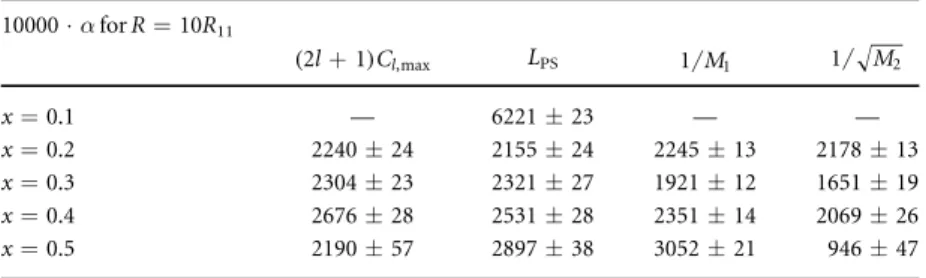
Power-law exponentsα obtained by linear fits to the domain growth stages ( *t >tc*) in figures3and6are

presented in table1for the large sphere and respectively in table2for the small sphere. Also thefit values for the power spectrum measures, the total power(2l+1)Cl,maxand the average domain size LPSare presented.

Uncertainties are given by thefit routine. Statistics generally are better for the MFs, in particular 1/M1gives the

smallest statistical errors and provides the most comparable curves to a power-law. The angular power spectral density based measures have high uncertainties and in particular for the small sphere they only provide few curves that allow for a power-lawfit.

The power-law exponents are found to be close toα ; 0.2. This is close to the predicted value in [42]. It is smaller than the value of 1/3 that is predicted in the diffusive domain growth regime of the Lifshitz–Slyozov growth law[29,43]. Only in the case of the mixture parameter x=0.5 the power-law exponent gets close to the prediction in the diffusive regime.

4.5. Hints towards universal behavior

Motivated byfindings in [3] universal features in the demixing behavior on spherical geometries are

investigated. We hypothesize that the temporal development of the structure parameters becomes independent of the mixture parameter and sphere size by a suitable rescaling of axis. The rescaled time *tr is a function

*= (* )

tr f t , ,x R and the rescaled measures mrare transformed viamr= (g M x R, , )for different measures M.

The specific scalings are obtained by empirically testing simple functions f and g. In order to remove possible scaling effects due to the mixture parameter x and the sphere size R, that influence the otherwise universal dynamics,the simplest rescaling functions are products of the form_{f t(} *_{, ,x R)}=_{t x}* w_{(R R )}W

11 and

= s S

( ) ( )

g M x R, , Mx R R11 with real exponentsw,W, ,s S Î. Wefind universal behavior for the MFs M0

and M1. This is presented infigure7where, after rescaling, the graphs for M0and M1coincide well for all sphere

sizes and mixture parametersx>0.1. The time axis was scaled by *t t*·x-2 3· (R R )

11 3 2. M0was scaled

by the mixture parameter asM0M0 xinfigure7(b). M1was scaled by the mixture parameter and the sphere

Radius asM1M1 x (R R11)0.8infigure7(c). This hints towards a universal demixing behavior for these systems. Only the graphs for x=0.1 show a different behavior due to their very late start of the demixing process

Table 1. Power-law exponentα during domain growth phase for the large sphere R=10R11.

Values are obtained via linear_{fits in the log–log plots in figures}3and6fort*>t_c*. 10000·α for R=10R11 + (2l 1)Cl,max LPS 1 M1 1 M2 x=0.1 — 6221±23 — — x=0.2 2240±24 2155±24 2245±13 2178±13 x=0.3 2304±23 2321±27 1921±12 1651±19 x=0.4 2676±28 2531±28 2351±14 2069±26 x=0.5 2190±57 2897±38 3052±21 946±47

Table 2. Power-law exponent_{α during domain growth phase for the small sphere R=2.5R}11. Values

are obtained via linearfits in the log–log plots in figures3and6fort*>t_c*. 10000·α forR=2.5R11 + (2l 1)Cl,max LPS 1/M1 1 M2 x=0.1 — — — — x=0.2 — 1320±160 792±29 1200±210 x=0.3 — — 1330±30 1000±200 x=0.4 — 1500±30 1894±32 2230±210 x=0.5 3254±38 4511±19 3052±21 —

and thus may have qualitatively different demixing behavior. The specific scaling of axis is obtained by empirical testing of simple functions.

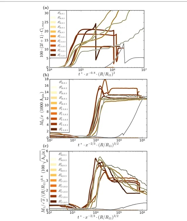
For the power spectral measures no rescaling of the axis could be found that leads to uniform graphs, see figure7(a). Since this could easily be achieved via MF measures this suggests that nonlinear properties play a role in the demixing process and that hence nonlinear measures, such as the MFs, are a more suitable means for the analysis of demixing processes.

5. Conclusion and outlook

An angular power spectrum analysis for DDFT calculations of the demixing processes on a sphere is able to detect different stages in the demixing process: the onset of spinodal decomposition, the main spinodal decomposition stage and the coalescence stage after spinodal decomposition. A scale-free power law growth

µ a

L t could be found for the domain size of demixed domains in the coalescence stage. The onset of the main Figure 7. After a rescaling of axis hints of universal behavior are found in panel(b) for M0and in panel(c) for M1. However, in panel

(a), no universal behavior is found for power spectral density(2l+1) ·Cl,max. Different sphere radii R and mixture parameters x are color coded. Their values are indicated in the legend by_{R R}2_{/ ,x}

112 .

spinodal decomposition phase is much later on the small sphere withR=2.5R11compared to the large sphere

withR=10R11. The same behavior is found for the crossover time between spinodal decomposition and

coalescence. Also the mixture parameter x influences these times: smaller x shifts the onset of the spinodal decomposition and also the crossover time to coalescence to later times. In the large sphere case many nucleation sites in the spinodal decomposition phase provide a large number of initially demixed domains. Thus during the growth and coalescence phase the domain size power law yields a smooth function. However, in the small sphere case only few nucleation sites exist and therefore also only few initially demixed domains exist after spinodal decomposition and prior to coalescence. This leads to a worse statistic in detecting the domain growth power law in the case of the small sphere.

The main spinodal decomposition stage cannot be detected with the standard method of analyzing the average domain size LPSprovided by the structure factor (S l t, ). This measure is only responsive to the domain

coalescence in the late stage of demixing. Using the maximum of the structure factor, the power(2l+1)Cl,max, one can observe the spinodal decomposition stage prior to the coalescence of domains. The MFs provide even further insight: they reveal that the main spinodal decomposition stage actually is composed of two parts: atfirst the functional measures M0and M1show a slow growth and after a specific value start to grow faster until the

beginning of the coalescence stage. MFs are able to resolve a further level of detail in the spinodal decomposition process. A systematic evaluation of the MFs on further demixing systems might shed new light on the early stage spinodal decompostion dynamics.

Another advantage of MFs is their scaling behavior during the coalescence stage: The domain growth power-laws are reproduced with higher precision than using the angular power spectrum method. The MFs seem to be a convenient measure to efficiently determine domain growth power-law exponents and shed light on a possible connection between the growth rate and the domain morphology.

The MFs allow the precise measurement of the mixture parameter x only observing the early stage spinodal decomposition without knowledge of the demixed end state. Since the density in the initial mixture is

r r_th,100 x, all relative threshold values below x result in almost no pixels being active after binarization, but almost all pixels are active for higher thresholds. This leads to a sharp transition of the value of the MFs at r_th r_th,100 x.

The most interesting new insight gained by a morphological MF analysis is their universal behavior. By applying a suitable rescaling, all MFs collapse onto a single master curve. The only exception being the curve for the smallest mixture parameter x=0.1, suggesting a qualitatively different demixing scenario with a much later onset of phase separation. For higher mixture parameters this shows that the analyzed demixing process has a universal, parameter independent domain evolution. For the angular power spectrum measures no suitable rescaling of the axis could be found. This suggests that nonlinear properties play an important role in the demixing process and thus that the inherently nonlinear MFs are a suitable tool for the characterization of this process. In further studies we will use surrogates[17–19] in order to disentangle the linear and nonlinear effects of the demixing process and their impact on the behavior of the MFs.

This result immediately suggest further analysis of the binary demixing system on spherical geometry: What are the differences between the low and high mixture parameter classes and how is the transition between these classes? Other questions worth of further examination are: Is this behavior influenced by the interaction potential, and is there a connection to theflat three-dimensional case?

Hints towards universal behavior in demixing systems via MF(and tensor) analysis were already discovered in previous studies[3]. Here simulations of a three-dimensional system with a binary complex plasma were analyzed. A universal behavior was found for different screening length rations of a double Yukawa interaction potential. There, also an exception of the universal behavior was found for a single screening length interaction potential. Further investigation of the universal behavior of demixing processes on various geometries, boundary conditions and with various interaction potentials are vital in order to obtain a thorough

understanding of the fundamental properties of demixing systems. The preliminary analyses in this work and in [3] suggest that further investigation will lead to deeper insight into the physical mechanisms of the demixing of binary systems.

Applying higher ranked(tensor) Minkowski valuations to demixing DDFT calculations on spherical geometries in further studies may shed further light on the features of the universal properties of the demixing process. Tensor MF on the two-sphere 2_{were introduced and applied in[44,45]. Higher ranked Minkowski}

tensor measures already proved to be useful in characterizing the solid–liquid phase transition in a two-dimensionalflat complex plasma [46]. Also the resolution of the DDFT calculations can be significantly improved in further studies.

This study gives further evidence that MF methods are a powerful tool for morphological characterization of physical processes. They are superior to conventional analysis methods in various respects: they directly provide information on the morphology of structures, are inherently nonlinear, and are fast and easy to compute (by only counting pixels) compared to correlation function measures. They allow the measurement of the

characteristic length scale L with high statistical reliability even for low resolution data. MF analysis is able to quickly reveal new aspects of interest in particular in nonlinear(non-Gaussian) data. It is founded on a solid mathematical framework, however it still provides easily interpretable results.

Acknowledgments

We thank I Laut for carefully checking this manuscript. AB was funded by the StMWi, MCB acknowledges funding provided by the Swiss National Science Foundation through the National Center of Competence in Research Bio-Inspired Materials.

ORCID iDs

A Böbel https://orcid.org/0000-0001-5612-7543

References

[1] Gunton J D, Miguel M and Sahni P S 1983 The dynamics of first order phase transitions Phase Transitions and Critical Phenomena ed C Domb and J Lebowitz_{(New York: Academic)}

[2] Bray A J 1994 Adv. Phys.43 357–459

[3] Böbel A and Räth C 2016 Phys. Rev. E94 013201

[4] Li W H and Lee J 1994 Phys. A: Stat. Mech. Appl.202 165–74

[5] Lee J 1994 Phys. A: Stat. Mech. Appl.210 127–38

[6] Bott M C and Brader J M 2016 Phys. Rev. E94 012603

[7] Guerra R E, Kelleher C P, Hollingsworth A D and Chaikin P M 2018 Nature554 346

[8] Soni V, Gómez L R and Irvine W T M 2018 Phys. Rev. X8 011039

[9] Krause A L, Burton A M, Fadai N T and Van Gorder R A 2018 Phys. Rev. E97 042215

[10] Stanley H E 1987 Introduction to Phase Transitions and Critical Phenomena (Oxford: Oxford University Press) [11] Allen M P and Tildesley D J 1987 Computer Simulation of Liquids (New York: Oxford University Press) [12] Wysocki A et al 2010 Phys. Rev. Lett.105 045001

[13] Velasco E and Toxvaerd S 1996 Phys. Rev. E54 605–10

[14] Mecke K R and Sofonea V 1997 Phys. Rev. E56 R3761–4

[15] Sofonea V and Mecke K 1999 Eur. Phys. J. B8 99–112

[16] Minkowski H 1903 Math. Ann.57 447–95

[17] Rossmanith G, Modest H, Räth C, Banday A J, Górski K M and Morfill G 2012 Phys. Rev. D86 083005

[18] Modest H I, Räth C, Banday A J, Rossmanith G, Sütterlin R, Basak S, Delabrouille J, Górski K M and Morfill G E 2013 Mon. Not. R. Astron. Soc.428 551_–62

[19] Modest H I, Räth C, Banday A J, Górski K M and Morfill G E 2014 Phys. Rev. D89 123004

[20] Stillinger F H 1976 J. Chem. Phys.65 3968

[21] Archer A J and Evans R 2001 Phys. Rev. E64 041501

[22] Louis A A, Bolhuis P G and Hansen J P 2000 Phys. Rev. E62 7961–72

[23] Archer A J and Evans R 2004 J. Chem. Phys.121 4246–54

[24] Marconi U M B and Tarazona P 1999 J. Chem. Phys.110 8032

[25] Driscoll J and Healy D 1994 Adv. Appl. Math.15 202–50

[26] Onuki A 2002 Phase Transition Dynamics (Cambridge: Cambridge University Press) [27]https://healpy.readthedocs.io

[28] Górski K M, Hivon E, Banday A J, Wandelt B D, Hansen F K, Reinecke M and Bartelmann M 2005 Astrophys. J.622 759

[29] Thakre A K, den Otter W K and Briels W J 2008 Phys. Rev. E77 011503

[30] Furukawa H 1984 Phys. A: Stat. Mech. Appl.123 497–515

[31] Weil W 1983 Stereology: A Survey for Geometers (Basel: Birkhäuser Basel) pp 360–412

[32] Schneider R 2013 Convex bodies: the Brunn-Minkowski theory Encyclopedia of Mathematics and its Applications 2nd edn (Cambridge: Cambridge University Press)

[33] Mecke K R, Buchert T and Wagner H 1994 Astron. Astrophys. 288 697–704

[34] Hadwiger H 1957 Vorlesungen über Inhalt, Oberfläche und Isoperimetrie (Berlin: Springer) [35] Helfrich W 1973 Z. Naturforsch.28c 693_–703

[36] Mecke K R 1996 Phys. Rev. E53 4794_–800

[37] Rosenfeld Y 1995 Mol. Phys.86 637–47

[38] Mecke K 2000 Additivity, convexity and beyond: applications of Minkowski functionals in statistical physics Statistical Physics and Spatial Statistics(Lecture Notes in Physics vol 554) ed K R Mecke and Stoyan D S (Berlin: Springer) pp 111–84

[39] Schmalzing J and Górski K M 1998 Mon. Not. R. Astron. Soc.297 355–65

[40] Winitzki S and Kosowsky A 1998 New Astron.3 75–99

[41] Michielsen K and Raedt H D 2001 Phys. Rep.347 461–538

[42] Binder K and Stauffer D 1974 Phys. Rev. Lett.33 1006–9

[43] Lifshitz I and Slyozov V 1961 J. Phys. Chem. Solids19 35–50

[44] Chingangbam P, Yogendran K, Joby P, Ganesan V, Appleby S and Park C 2017 J. Cosmol. Astropart. Phys.2017 023

[45] Ganesan V and Chingangbam P 2017 J. Cosmol. Astropart. Phys.2017 023