HAL Id: hal-01026308
https://hal.archives-ouvertes.fr/hal-01026308
Submitted on 21 Jul 2014
HAL is a multi-disciplinary open access
archive for the deposit and dissemination of
sci-entific research documents, whether they are
pub-lished or not. The documents may come from
teaching and research institutions in France or
abroad, or from public or private research centers.
L’archive ouverte pluridisciplinaire HAL, est
destinée au dépôt et à la diffusion de documents
scientifiques de niveau recherche, publiés ou non,
émanant des établissements d’enseignement et de
recherche français ou étrangers, des laboratoires
publics ou privés.
A fictitious domain approach for the simulation of dense
suspensions
Stany Gallier, Elisabeth Lemaire, Laurent Lobry, François Peters
To cite this version:
Stany Gallier, Elisabeth Lemaire, Laurent Lobry, François Peters. A fictitious domain approach for the
simulation of dense suspensions. Journal of Computational Physics, Elsevier, 2014, 256, pp.367-387.
�10.1016/j.jcp.2013.09.015�. �hal-01026308�
A fictitious domain approach for the simulation of dense suspensions
Stany GALLIERa,b,⇤, Elisabeth LEMAIREb, Laurent LOBRYb, Franc¸ois PETERSb
aSAFRAN-Herakles, Le Bouchet Research Center, 91710 Vert le Petit, France bCNRS, University of Nice LPMC, UMR 6622, Parc Valrose, 06108 Nice, France
Abstract
Low Reynolds number concentrated suspensions do exhibit an intricate physics which can be partly unraveled by the use of numerical simulation. To this end, a Lagrange multiplier-free fictitious domain approach is described in this work. Unlike some methods recently proposed, the present approach is fully Eulerian and therefore does not need any transfer between the Eulerian background grid and some Lagrangian nodes attached to particles. Lubrication forces between particles play an important role in the suspension rheology and have been properly accounted for in the model. A robust and effective lubrication scheme is outlined which consists in transposing the classical approach used in Stokesian Dynamics to our present direct numerical simulation. This lubrication model has also been adapted to account for solid boundaries such as walls. Contact forces between particles are modeled using a classical Discrete Element Method (DEM), a widely used method in granular matter physics. Comprehensive validations are presented on various one-particle, two-particle or three-particle configurations in a linear shear flow as well as someO(103) and O(104) particle simulations.
Keywords:
Suspensions, Fictitious domain, Lubrication, Discrete Element Method
1. Introduction
Suspensions of solid particles embedded in a liquid are a class of two-phase flows that are ubiquitous in industry as well as in biological or natural flows. Fresh concrete or uncured solid rocket fuel are two examples of industrial concentrated suspensions for which the highest particle volume fraction is desired while keeping correct rheological properties and flowing behavior. Such dense suspensions do exhibit an intricate physics which is hitherto far beyond complete understanding. This complexity mainly stems from the wide variety of fluid-particle or particle-particle interactions [1] so that even the idealized case of hydrodynamically-interacting smooth monodisperse spherical par-ticles in a Newtonian fluid can involve strong non-Newtonian effects such as yield stress, shear-thickening, particle migration or anisotropic microstructures (see [2, 3] for a review).
⇤Corresponding author. Tel.:+33 1 64991193 ; fax:+33 1 64991118.
Email address: stany.gallier@herakles.com (Stany GALLIER)
*Manuscript
The development of numerical simulation can help shed light on the complex physics of suspensions. However, due to the importance of flow-particle interactions, only microscale methods – wherein the flow is fully resolved around each particle – are relevant. In contrast, macroscale methods are less computationally demanding but require a local averaging – because computational cells are much larger than particles – which loses the essential details of the flow. For low Reynolds number suspensions, well-suited techniques include Stokesian Dynamics (SD) [4–7] and Force-Coupling Method (FCM) [8–10]. Although different, both methods rely on a truncated multipole expansion so-lution of the Stokes equations. They undoubtedly have numerous upsides and appear to be instrumental in providing among the most influential results in the field of suspension physics. Nevertheless, they are highly specialized and may not tackle any kind of flows. Because they rest on special solutions of the Stokes equations (multipole expan-sion), they are inherently restricted to non- or weakly-inertial flows. By and large, multipole expansions are mostly available for spheres, thereby preventing from simulating arbitrary-shaped particles. Furthermore, it is not possible to consider non-Newtonian fluids with these techniques. Therefore, direct numerical simulation (DNS) has emerged as an attractive alternative. In this approach, governing equations (Navier-Stokes or Stokes equations) are solved without any further assumptions other than numerical approximations. This makes possible to solve particulate flows with arbitrary particle shape, flow Reynolds number or fluid rheological constitutive equation. The very first class of DNS methods dedicated to particulate flows followed a boundary-fitted approach wherein only the domain occupied by the fluid is meshed [11, 12]. As particles move, the constantly evolving fluid domain poses complex remesh-ing issues. For sheared concentrated suspensions, in which particle separation can be vanishremesh-ingly small, remeshremesh-ing becomes extremely involved and makes this approach impractical for more than a few particles. As an exception, let us mention the works of Johnson and Tezduyar [13] who performed impressive 3D simulations with up to 100 particles with such body-fitted techniques. In contrast, non-boundary-fitted methods are much more suited for the simulation of suspensions with a large number of particles. The whole domain is mapped onto an Eulerian fixed grid and particles are embedded in this regular non-moving grid. Non-boundary-fitted methods for particulate flows in-clude different techniques, such as immersed boundary methods [14–16], fictitious domain methods [17–19] or lattice Boltzmann methods [20–22]. Fictitious domain methods have met considerable interest and have been widely used so far [23–27]. They have been successfully applied to non-Newtonian flows [28–31], heat transfer in suspensions [32] or non-spherical particles such as ellipsoids [25], cubes [24], polygons [33], plates [23] or fibers [34]. Fictitious domain methods are generally body-force-based methods since solid particles are modeled via a body-force (or mo-mentum forcing) introduced in the momo-mentum equation to enforce a rigid body motion. There exist various methods to handle this body-force and a review is provided in Yu and Shao [25]. In the original fictitious domain approach by Glowinski et al. [17, 18, 35], the body-force is introduced as a Lagrange multiplier in a weak formulation and solved in an iterative way. However, the method is computationally expansive as a saddle-point problem must be solved. Patankar’s works [23, 36] were the first to develop a non-Lagrange multiplier version of fictitious domain in order to improve computational performance. More recent studies [24–26] have still continued in this way of non-Lagrange multiplier methods by working out an explicit equation on the body-force. These previously cited studies share many
similarities and only slightly differ.
Surprisingly, despite the availability of these DNS methods, quantitative simulations of dense suspensions are heretofore a privilege of SD or FCM methods. Only scarce studies address the DNS of suspension rheology [25, 28, 29, 37] but they remain mostly qualitative and far from actual configurations as they consider 2D particles (cylinders) with low volume fractions. As far as the authors know, there have been no attempts at simulating the rheological be-havior of dense suspensions using DNS in the way it is done by SD or FCM. With an eye to demonstrating that DNS is well-adapted for detailed simulations of concentrated suspensions, this study intends to develop a non-Lagrange multiplier version [24, 25] of the fictitious domain approach since it alleviates the computational burden of the orig-inal version. However, those methods define body-force values at some Lagrangian nodes attached to the particles moving in the Eulerian background grid. This consequently involves several interpolation steps between Eulerian and Lagrangian nodes, which are known to induce numerical instabilities [25] and impose a careful choice of the interpolation kernel [14, 38]. It is also attested that the arrangement itself of the Lagrangian particle nodes may alter results. For spheres, the best results are obtained with nodes adequately arranged in concentric shells and with the nodes closest to the particle surface slightly retracted from it [25, 39]. A generalization to arbitrary-shaped particles is believed to be tedious. Therefore, our approach intends to keep the simplicity of a fully Eulerian method. Body-force quantities are defined at the Eulerian grid points, like the other fluid variables, and an Eulerian advection step is inserted in the method, so that the body-force remains attached to the particle as it moves along.
A peculiar feature of concentrated suspensions is that the average separation distance a⇠ between particles, where
adenotes the particle radius, becomes extremely small. The so-called lubrication forces arise between particles in near-contact because of the draining of interstitial fluid in the gap. The magnitude of these forces rises dramatically as particles approach each other and is singular in the limit of touching particles as the normal and tangential forces diverge as ⇠−1and ln ⇠, respectively. Consequently, the rheology of suspensions is markedly modified by lubrication forces and qualitatively important effects occur at small separations, typically down to ⇠ ⇠ 10−2. For accurate sim-ulations of low Reynolds suspensions, a numerical method should be able to capture those short-range lubrication forces. The required grid spacing should however be smaller than at least 10−3a–10−4ato resolve lubrication, making long-term simulations of many-particle systems unfeasible. Typical grid spacings are about 10−1awhich means that – albeit implicitly accounted for by DNS – lubrication forces are less and less accurately described as particles come to near contact. A first simple approach consists in adding the theoretical lubrication force Fthlub(⇠), known for two spheres in near-contact [40], to the computed hydrodynamic force. To put it more precisely, this rather takes the form Fth
lub(⇠)− F th
lub(⇠cut) where ⇠cutis a cut-off separation below which this lubrication correction is activated. This approach is widely employed whatever the numerical technique chosen : fictitious domain [32], dissipative particle dynamics [41], lattice Boltzmann method [42] or boundary element method [43]. Yet, such simple approach is not rigorous because – as previously stressed – a part of the lubrication is already partially included in the numerical solution. Just adding the theoretical force consequently results in double-counting the resolved part of the lubrication force. A more rigorous method is proposed in SD [6, 44]. The analytical two-sphere resistance interactions are added
to the long-range hydrodynamic resistance matrix. However, in order not to count twice the far-field part of the exact two-sphere resistance interactions, the authors subtract off this contribution, which is found by inverting a two-sphere mobility matrix to the same level of approximation as in the long-range hydrodynamic problem. This method is however not well suited for DNS because long-range hydrodynamic resistance or mobility matrices are not explicitly computed. In the frame of FCM, Maxey et al. [10, 45] developed an approach inspired by the method used in SD. The main idea is to compute, without any lubrication correction, the interactions between two spheres for different configurations and separation distances ⇠, in order to estimate the numerically resolved part of lubrication. The basic ideas of this method can be retained and readily transposed to a DNS approach, which will be done in the frame of this study. Note that there exist other alternatives such as using X-FEM (Extended Finite Element Method) to enrich the solution with lubrication theory in order to capture the subgrid-scale lubrication layer flow [46]. This is an earlier example of a combination of DNS and lubrication (while avoiding double-counting) but was only demonstrated in 2D and for small numbers of particles (⇠10).
A last essential ingredient for accurate simulations of suspension physics is the modeling of collisions, or contacts, between particles. Contacts inevitably occur in inertial flows but also in non-inertial flows despite lubrication because of many-body interactions or particle roughness. Additionally, from a numerical standpoint, contact may also take place in dense suspensions due to finite time steps. In order to prevent from unphysical particle overlaps, most authors include an additional ad hoc short-range repulsion force. The functional form of this force is usually dictated by numerical convenience rather than physics. Nonetheless, the important role of contact forces in dense suspensions has been highlighted in recent experimental works that unequivocally show that moderately-sheared highly-concentrated suspensions behave like dry granular materials (e.g., see [47]). As dry granular materials have long been known to be well modeled by a Discrete Element Method (DEM) (see [48, 49] for a review), couplings between DEM and DNS solvers have recently emerged [33, 50]. Yet, those works do not consider lubrication and a peculiar feature of our present model is that both lubrication and contact using DEM are considered.
The goal of this paper is to present an efficient method suited for the simulation of concentrated suspensions, thereby including a detailed modeling of lubrication and contact. Section 2 describes the fictitious domain method employed. It is close to the works of Yu and Shao [25] and Apte et al. [24] although a significant difference is that our method is fully Eulerian and does not require Lagrangian collocation nodes. In Section 3, a robust and effective lubrication method is presented. It retains the basic ideas of the recent method proposed in FCM [10] and is adapted to the present DNS approach. In Section 4, the DEM method is delineated. Section 5 presents different comprehensive validations especially focusing on spheres in linear shear flows. Finally, conclusions are given in Section 6.
2. Fictitious domain method
2.1. Governing equations
LetD be the computational domain including the fluid domain Df and the solid particle domain Dp, so that D = Df ⊕ Dp. The particle domain is assumed to be made up of N particlesPi : Dp = Si=Ni=1 Pi. In the frame of the present work, particles are assumed to be rigid and homogeneous with density ⇢p. The boundary between fluid and particle domains is noted @P. The idea of fictitious domain is to extend the Navier-Stokes equations in the whole domainD including particles. They are thus supposed to be filled with the fluid, which is supposed here to be Newtonian and incompressible with density ⇢f and viscosity µ. Incompressibility for velocity u in the whole domain D yields
r · u = 0 (1)
whereas the momentum equation in the whole domainD reads: ⇢f(
@u
@t +u· ru) = r · Σ + ⇢fλ (2)
where the term ⇢fλcan be seen as a body-force that enforces the rigid body motion inside particles. This force is non-zero in the particle domainDpand zero in the fluid domainDf. The fluid stress tensor Σ reads for a Newtonian fluid :
Σ =−pI + 2µE (3)
where p is the fluid pressure and E the rate-of-strain tensor E = 12(ru + ruT
). Note that in Eq. (2), gravity is not included since the whole domainD is filled with the same fluid of density ⇢f. Buoyancy forces will be included in a subsequent step. Particles are supposed to be rigid, so that the velocity field inside particles is given by a rigid body motion
u = U + Ω⇥ r (4)
where U and Ω are the particle translational and rotational velocities, respectively, and r denotes the position vector with respect to particle center of gravity r = x− xG.
The forthcoming developments intend to construct some explicit expressions for particle velocities and forcing term λ and are close to Yu and Shao [25]. Particle motion is given by Newton’s equations and reads
MdU dt =F hyd+ (1−⇢f ⇢p )Mg + Fint (5) J.dΩ dt + Ω⇥ (J.Ω) = T hyd+ Tint (6)
where g is the gravity acceleration and Fintand Tintare the force and torque due to interactions on particles. In present work, they will describe the contact between particles but they also can represent any other external interactions such as electrostatic forces for instance. Fhydand Thyd are respectively the hydrodynamic force and torque exerted by the fluid on the particle :
Fhyd= Z @Pn.Σ dS (7) Thyd= Z @P r⇥ (n.Σ) dS (8)
where n is the outward-pointing unit normal vector on the boundary @P. In Eq. (5) and Eq. (6), M and J stand for the particle mass and inertia tensor :
M = Z P ⇢ dx (9) J = Z P ⇢[(r.r)I− r ⌦ r] dx (10)
These integrals are easily handled by introducing a generalized density ⇢(x) given as
⇢(x) = ⇢f(1− IP(x)) + ⇢pIP(x) (11)
whereIP(x) is the particle indicator function:
IP(x) = 8 > > > > > < > > > > > : 1 if x2 P 0 if x <P (12)
Integrating momentum equation Eq. (2) as well as r⇥ Eq. (2) on a particle P and using the rigidity constraint Eq. (4) and the definition of hydrodynamic force Eq. (7) and torque Eq. (8) yields
Fhyd=−⇢f Z P λdx +⇢f ⇢p MdU dt (13) Thyd=−⇢f Z P r⇥ λ dx +⇢f ⇢p ⇥J.dΩ dt + Ω⇥ (J.Ω) ⇤ (14) Using these expressions in Eq. (5) and Eq. (6) provides
⇢f Z P λdx =(⇢f − ⇢p) ⇢p M[dU dt − g] + F int (15) ⇢f Z P r⇥ λ dx = (⇢f − ⇢p) ⇢p ⇥J.dΩ dt + Ω⇥ (J.Ω)⇤ + T int (16) Eventually, the fluid-particle problem is governed by the following equations
@u @t +u· ru = − rp ⇢f +⌫r2u + λ inD (17) r · u = 0 inD (18) u = U + Ω⇥ r inDp (19) ⇢f Z P λdx = (⇢f− ⇢p) ⇢p M[dU dt − g] + F int (20) ⇢f Z P r⇥ λ dx = (⇢f− ⇢p) ⇢p ⇥J.dΩ dt + Ω⇥ (J.Ω)⇤ + T int (21)
where ⌫ = µ/⇢f is the fluid kinematic viscosity. At this step, the governing equations are essentially similar to the ones proposed by Yu and Shao [25] and Apte et al. [24] and are a strong-form counterpart of the classical fictitious domain method introduced by Glowinski et al. [17, 18, 35]
2.2. Numerical procedure
A fractional-step time scheme is used to decouple the previous system Eq. (17)-(21) into two subproblems. The first subproblem Eq. (17)-(18) is a standard Navier-Stokes problem inD whereas Eq. (19)-(21) form a particle sub-problem which mainly consists in enforcing the rigid body motion inside particles. The numerical procedure is presented for the general case of 3D flows with arbitrary-shaped particles although only spheres will be considered in this paper.
2.2.1. Fluid subproblem
The standard incompressible Navier-Stokes equations Eq. (17)-(18) are classically solved using finite differences on half-staggered Cartesian grids. The whole domainD is uniformly meshed with a constant grid spacing ∆. The components of the forcing term λ are half-staggered in the same way as the velocity components. As we primarily focus on low Reynolds number flows, the time integration scheme is implicit (Crank-Nicolson) for the diffusive terms and explicit for the convective terms using a second-order Adams-Bashforth scheme :
un+1 − un ∆t +[ 3 2(u· ru) n −12(u· ru)n−1] +rp n+1 ⇢f = ⌫ 2r 2 (un+1+un) + λn (22) r · un+1=0 (23)
This formulation is similar to the non-Lagrange multiplier methods already mentioned [24–26] and differs from the original fictitious domain method [17, 18, 35] in the sense that the rigid body motion is here imposed only in an approximate way because the forcing at the previous iteration λn is used. The system Eq. (22)-(23) is classically solved using a projection method [51, 52]. In such approach, the momentum equation Eq. (22) is first solved while discarding the pressure term (i.e.rpn+1=0). The obtained velocity field, noted u⇤, is consequently not divergence-free (r · u⇤,0). The subsequent projection step is obtained on noting that
u⇤=un+1+∆t ⇢f rp
n+1
(24) which is an Helmoltz-Hodge decomposition of velocity u⇤. Taking the divergence of Eq. (24) and imposing a divergence-free condition for velocity un+1gives a Poisson equation on the pressure
r2pn+1 =⇢f ∆tr · u
⇤ (25)
The resulting pressure field pn+1is then used in Eq. (24) so as to obtain the desired velocity un+1.
The space discretization of gradient or laplacian operators is achieved using classical second-order centered schemes. The four resulting linear systems (three for each velocity component in Eq. (22), one for pressure in Eq. (25)) are solved by a geometric multigrid with V-cycles and two Gauss-Seidel iterations for pre- and post-smoothing.
2.2.2. Particle subproblem
The particle subproblem is three-fold : first, constrain a rigid body motion inside particles ; second, compute particle velocities ; and third, update the forcing term λ. As previously stressed, the fluid velocity un+1 does not exactly comply with a rigid body motion inside particles because the used forcing term λnis taken at the previous time step. At this stage, an explicit direct forcing of the rigid body motion is thus required :
˜un+1=Un+1+ Ωn+1⇥ r inDp (26)
This new velocity ˜un+1 now fulfills an exact rigid body motion inside particles. It can be noted that the difference between ˜un+1 and un+1 is a measure of the defect in constraining the exact rigid body condition and can be used to update λ. To this end, the discretized Navier-Stokes equation Eq. (22) can be rewritten in the following compact form
un+1 − un
∆t =r · F n+1
+ λn (27)
The new velocity ˜un+1describes an exact rigid body motion, so that ˜un+1 − un ∆t =r · ˜F n+1 + λn+1 (28) By difference, we obtain λn+1 = λn+ ˜u n+1 − un+1 ∆t − r · ( ˜F n+1 − Fn+1) (29)
Rigorously speaking, fluxes ˜Fn+1and Fn+1are not exactly equal because velocities have been slightly modified due to the correction step Eq. (26). Indeed, ˜Fn+1is not explicitly known and depends on λn+1so that Eq. (29) is an implicit equation of limited practical interest. In order to have an explicit equation on λn+1, the following approximation is used
˜
Fn+1⇡ Fn+1 (30)
which is a reasonable assumption for moderate time steps. This eventually gives a simple explicit equation for the forcing term :
λn+1 = λn+ ˜u
n+1− un+1
∆t (31)
The last step consists in computing the particle translational and rotational velocities Un+1
and Ωn+1that are actually required to enforce the rigid body motion Eq. (26). The discretized counterparts of Eq. (20) and Eq. (21) read
⇢f Z P λn+1dx =(⇢f − ⇢p) ⇢p M[U n+1 − Un ∆t − g] + F int,n (32) ⇢f Z P r⇥ λn+1dx =(⇢f − ⇢p) ⇢p [J.(Ω n+1 − Ωn) ∆t + Ω n ⇥ (J.Ωn)] + Tint,n (33)
Substituting Eq. (26) in Eq. (31) gives
λn+1= λn+U
n+1+ Ωn+1
⇥ r − un+1
Finally, Eq. (34) is integrated on the particle volume and inserted in Eq. (32) and, similarly, r⇥ Eq. (34) is integrated and inserted in Eq. (33). This leads to the explicit equations
MUn+1= (⇢p− ⇢f) ⇢p M[Un+g∆t] + ⇢f Z P (un+1− λn∆t) dx + Fint,n∆t (35) J.Ωn+1= (⇢p− ⇢f) ⇢p [J.Ω n − Ωn ⇥ (J.Ωn )∆t] + ⇢f Z P r⇥ (un+1 − λn ∆t) dx + Tint,n∆t (36)
Let us remark that in the general case of non-spherical particles, the inertia tensor J is not diagonal which requires an additional 3⇥3 system inversion in Eq. (36) so as to compute the rotational velocities. These expressions for velocities are essentially similar to the ones obtained by other non-Lagrange multiplier techniques [24–26].
2.3. Particle tracking
Non-boundary-fitted Eulerian methods are attractive since a fixed mesh avoids any remeshing difficulties. How-ever, the interface between fluid and particles must be defined properly. A large amount of work is devoted to this interface tracking problem, such as VOF (Volume-Of-Fluid) methods [53] or level-set methods [54, 55] (see also [56] for a review.) Still, this problem is not acute here because only rigid particles are considered and their shape conse-quently remains unchanged. In present case, the interface tracking is needed so as to delineate the fluid regionDf and the particle regionDp. The method chosen here rests on the well-known level-set approach [54, 55] which considers a level-set function (x) negative inside particles and positive outside and with the interface defined by the hypersurface (x)=0. A widely employed level-set function is the signed distance : for the simple case of a sphere of radius a centered at xG, the level-set reads
(x) =kx − xGk − a (37)
The previously introduced particle indicator functionIP(x) can be directly computed from the level-set function :
IP(x) = 1− H( (x)) (38)
where H is the Heaviside function
H(s) = 8 > > > > > < > > > > > : 0 if s 0 1 if s > 0 (39)
This Heaviside function is smeared over a small region ✏ (proportional to grid spacing) around the boundary giving a smooth variation that will enhance numerical accuracy and robustness, such as
H✏(s) = 1
2(1 + tanh(b
s
∆)) (40)
where ∆ is the grid spacing and b is a free parameter controlling the smearing on a typical size ✏ ⇠ O(∆/b). In the present study, a value b=5 is chosen which gives a correct smoothing in typically less than a grid spacing. The
corresponding smooth indicator functionI✏
Pis then used to compute the particle mass, volume, inertia tensor as well as any integral of a quantity φ on the particle volumeP
Z P φ dx = Z D(P)I ✏ P(x).φ dx (41)
where the integration domainD(P) is a subset of D encompassing the particle P (bounding box).
Particles are assumed to be rigid so that their position can be tracked by solving the following transport equation dX
dt =U (42)
where X denotes the vector of particle centers. For non-spherical particles, X also contains orientations (Euler angles or quaternions) and U additionally includes rotational velocities. Note however that the present study will only focus on spheres. Using a second-order Adams-Bashforth scheme, the previous equation reads
Xn+1=Xn+3 2∆tU n+1 −1 2∆tU n (43) A peculiar feature of our approach is to be fully Eulerian : the forcing λ is not defined at some particle collocation nodes but rather at the Eulerian grid points like any other fluid variables. Consequently, an Eulerian transport step is inserted in the method so that the forcing remains attached to the moving particle. Hence, the following advection equation is solved for each particleP
@λP
@t +UP.rλP=0 (44)
where subscriptP has here been added to recall that this equation needs to be solved for each particle. Practically speaking, this equation is solved only in the bounding boxD(P) to avoid unnecessary computational effort. Equa-tion (44) is a classical advecEqua-tion equaEqua-tion for which a large number of methods is available. However, the forcing term λ
Phas a very sharp variation across the particle boundary (it is zero in the fluid domain) and even high-order schemes, such as a fifth-order WENO (Weighted Essentially Non-Oscillatory) scheme [57] or a fourth-order WKL (Warming-Kutler-Lomax) scheme [58], failed to correctly advect the forcing on moderately coarse grids without any appreciable dissipation and dispersion. The best performance is found to be obtained by semi-Lagrangian schemes [58–60] that are furthermore ideally suited for Cartesian grids. The advection step Eq. (44) is written in Lagrangian form DλP/Dt = 0 which means that quantity λPis conserved on the characteristic path dx/dt = UP. The semi-Lagrangian scheme then simply reads
λ
P(x, t + ∆t) = λP(x− UP∆t, t) (45)
which just requires an interpolation of the forcing at position x−UP∆t. The overall accuracy of the scheme is governed by the accuracy of this interpolation. Although (tri-)linear interpolation is simple, it induces much dissipation. A second-order Lagrange polynomial interpolation is preferred as a good trade-off between accuracy and computational demand. Note that this semi-Lagrangian scheme is reminiscent of high-order Lagrangian/Eulerian interpolation steps in usual fictitious domain methods as discussed in the introduction. However, present interpolation step is performed only once per time step, just for advecting the momentum forcing, whereas three Lagrangian/Eulerian interpolation steps are generally required per iteration in the aforementioned methods (e.g., see [25]).
2.4. Numerical algorithm
The following steps are performed (where n is the current iteration) : 1. Compute level-set function
For each particleP, define a cubic bounding box D(P) encompassing the particle and compute the level-set function n
P(x) Eq. (37) and associated smeared indicator functionI ✏,n
P (x) in the bounding box 2. Advect momentum forcing
For each particleP, advect the forcing term from λn
to λn⇤by solving the transport equation Eq. (44) inD(P) for one time step ∆t
3. Solve fluid subproblem
Compute new fluid velocities un+1and pressure pn+1(Eq. (22) and Eq. (23)) using λn
⇤as the momentum forcing. 4. Update particle velocities
Update particle translational Un+1
and rotational velocities Ωn+1 using Eq. (35) and Eq. (36) with λn
⇤ as the momentum forcing and with interaction forces/torques Fint,n=Fint(Xn, Un) and Tint,n=Tint(Xn, Un).
5. Enforce rigid body motion
Explicitly enforce the rigid body motion ˜un+1=Un+1
+ Ωn+1⇥ r (Eq. (26)) inside each particle 6. Update momentum forcing
Correct the momentum forcing using Eq. (31) : λn+1= λn⇤+( ˜un+1− un+1)/∆t 7. Update particle position
Update particle position using Eq. (43) : Xn+1=Xn+3 2∆tU
n+1
−12∆tU
n 8. Repeat
Set n to n+1 and go to step 1
A last remark concerns the steady Stokes equations that will be extensively used in the forthcoming validations due to the availability of analytic solutions in this regime. Rather than considering extremely large fluid viscosity to obtain vanishing Reynolds numbers – which would inevitably result in a significant time step reduction despite the implicit time-stepping – it is preferred to discard the convective term (u· ru) in the Navier-Stokes equations. Furthermore, we loop over step 3 to 6 in pseudo-time until convergence before moving to the next steps. This actually consists in reaching a steady state Stokes flow before updating particle positions. This steady state is typically achieved within 2-3 subiterations.
3. Lubrication model
As stressed in the introduction, lubrication forces play a major role in the suspension rheology and need to be modeled properly. Since they are short-range in nature, they can usually not be fully resolved with the typical grids used and consequently require an ad hoc model. The method proposed is partly inspired from Stokesian Dynamics [6, 44] but has been here adapted to comply with a DNS framework.
3.1. Theoretical framework
Let us consider a system of N spherical particles suspended in a linear Stokes flow and let U be the 6N vector of translational/rotational velocities U = (U, Ω)T and F = (F, T)T the 6N vector of hydrodynamic forces/torques exerted by the fluid on the particles. Due to the linearity of the Stokes equations, there are linear relations between the forces/torques and the flow parameters and the velocities of particles can be written in resistance form as [40]
F = RFU· (U1− U) + RFE: E1 (46)
where U1and E1are the unperturbed velocities and the rate-of-strain tensor due to the prescribed flow field, respec-tively. The 6N⇥ 6N resistance matrices RFUet RFEare not known in general except for the case of two spheres. The key idea is to split the hydrodynamic interactions into long-range interactions – explicitly resolved by the numerical model – and a short-range lubrication contribution which can not be resolved since it is subgrid :
R ⇡ ˜R + Rsub
(47) where the tilde denotes the resolved part and the superscript sub refers to the subgrid unresolved part of the interaction. Expanding Eq. (46) together with Eq. (47) yields
U1− U = ˜R−1FU· [F − ˜RFE: E1− RsubFU· (U1− U) − RFEsub: E1] (48) The resolved velocity ˜U which is given by the numerical simulation formally reads
U1− ˜U = ˜R−1FU· [F − ˜RFE: E1] (49)
Combining Eq. (48) and Eq. (49) gives the exact velocity U in terms of the numerically resolved velocity ˜U U = ˜U + ˜R−1FU· [RFUsub· (U1− U) + RsubFE: E1] (50) This basically means that the lubrication-corrected velocity U can be obtained from the resolved velocity ˜U by adding the external force Flubin the numerical procedure with
Flub=RsubFU· (U1− U) + RsubFE : E1 (51)
This force represents the portion of hydrodynamic interactions not resolved by the numerical approach. The subgrid resistance matrices RsubFEand R
sub
FUwill be specified subsequently.
3.2. Numerical procedure
Newton’s equations for particles read
M·dU
where Fhyd represents the resolved hydrodynamic interactions (including gravity), Flub the additional lubrication force Eq. (51), Fint the contact interactions, and M the generalized mass/inertia matrix. Lubrication forces strongly depend on particle positions and velocities and are only weakly coupled with long-range hydrodynamics, so that Eq. (52) can be split into
M· U − U˜ n ∆t =Fhyd+Fint (53) M·U n+1 − ˜U ∆t =Flub (54)
The first step Eq. (53) corresponds to the numerical procedure to compute particle velocity and is a formal rewriting of Eqs. (35)-(36) while the second step Eq. (54) intends to correct the obtained particle velocity from lubrication. Since lubrication forces are very short-range, Eq. (54) is stiff and must be solved implicitly using Flub(Un+1). Rearranging Eq. (54) with Eq. (51) yields
[M ∆t+R sub FU]· U n+1= M ∆t· ˜U + R sub FU· U1+RsubFE : E1 (55)
From the known uncorrected velocity ˜U, the actual lubrication-corrected particle velocity Un+1
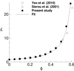
is obtained by solving the linear system Eq. (55). Since the resistance matrix RsubFU is symmetric and sparse, an iterative conjugate gradient method is used to solve the system until a prescribed relative tolerance is achieved (typically 10−6). By and large, iterative techniques work well for matrices that are well-conditioned (i.e., with eigenvalues tightly clustered). However, resistance matrices are generally ill-conditioned due to the singular behavior of the resistance functions near contact, which induces very poor convergence, if any. Therefore, a preconditioned conjugate gradient with an incom-plete Cholesky factorization with zero fill-in IC(0) is used. The efficiency of the preconditioning is further improved by a matrix reordering using a Reverse Cuthill-McKee (RCM) algorithm. As already noticed by Sierou and Brady [7], the preconditioned iterative procedure works well when the resistance matrix is reasonably well-behaved, in practice when the inter-particle distance is typically no less than 10−6a. As a result, a threshold distance of 10−6ais prescribed when constructing the resistance matrix with an eye to avoiding poor convergence rates.
In the numerical algorithm already presented (see Sec. 2.4), this lubrication correction step is performed just after the computation of particle velocities (step 4) and is therefore inserted between step 4 and step 5.
3.2.1. Subgrid resistance matrix
The subgrid resistance matrices RsubFUand R sub
FEdo represent the portion of hydrodynamic interactions not resolved by the numerical procedure. Just like in SD, subgrid resistance matrices are estimated by subtracting the two-body resistance matrices ˜R2Bobtained numerically from the exact two-body resistance matrices R2B,theoknown from lubri-cation theory :
For two spherical particles (1) and (2), the theoretical resistance relation for the force and torque is [40] 2 6 6 6 6 6 6 6 6 6 6 6 6 6 6 6 6 6 6 6 6 6 6 6 4 F1 F2 T1 T2 3 7 7 7 7 7 7 7 7 7 7 7 7 7 7 7 7 7 7 7 7 7 7 7 5 =µR2B,theo 2 6 6 6 6 6 6 6 6 6 6 6 6 6 6 6 6 6 6 6 6 6 6 6 6 6 6 6 6 6 6 6 6 6 6 6 6 6 6 4 u1(x1)− U1 u1(x2 )− U2 !1(x1)− Ω1 !1(x2)− Ω2 E1 E1 3 7 7 7 7 7 7 7 7 7 7 7 7 7 7 7 7 7 7 7 7 7 7 7 7 7 7 7 7 7 7 7 7 7 7 7 7 7 7 5 (57) with R2B,theo= 2 6 6 6 6 6 6 6 6 6 6 6 6 6 6 6 6 6 6 6 6 6 6 6 4 A11 A12 (B11)t (B21)t G11 G21 A12 A22 (B12 )t (B22 )t G12 G22 B11 B12 C11 C12 H11 H21 B21 B22 C12 C22 H12 H22 3 7 7 7 7 7 7 7 7 7 7 7 7 7 7 7 7 7 7 7 7 7 7 7 5 (58)
The various resistance tensors can be written in terms of several scalar functions [40]
A↵βi j = X↵βAdidj+ Y↵βA(δi j− didj) (59) B↵βi j = Y↵βB✏i jkdk (60) C↵βi j = XC↵βdidj+ YC↵β(δi j− didj) (61) G↵βi jk= XG↵β(djdk− 1 3δjk)di+ Y G ↵β(djδik+ dkδi j− 2didjdk) (62) H↵βi jk= Y↵βH(✏jildldk+✏kildldj) (63)
in which d = r/krk and r is the separation vector between particle centers r = x1− x2. In the previous expressions, δand ✏ stand for the Kronecker and Levi-Civita tensor, respectively. The different scalar functions X↵βand Y↵β in Eq. (59)-(63) depend on radius a and non-dimensional distance ⇠ = krk/a − 2, and their analytic forms are given in [40, 61].
In order to calculate ˜R2B, it is first assumed that this resistance tensor has the same functional form as the the-oretical R2B,theohereinbefore given by Eq. (58)-(63). The associated resolved scalar functions ˜X↵βand ˜Y↵βare then computed with our DNS solver – without any lubrication correction – for pairs of particles having various configura-tions (orientation and separation distance). The obtained resolved scalar funcconfigura-tions are subsequently tabulated against the non-dimensional separation distance ⇠. This step is done once for all. From a numerical viewpoint however, the solution slightly differs depending where the gap is located on the grid, especially if a coarse grid is used. For exam-ple, for two particles separated by one grid length, the computed lubrication force is different depending on whether the gap is spanned by a single grid cell, compared with two half-cells. In order to limit those grid-induced effects, the tabulated scalar functions are averaged over several configurations (for a given gap ⇠) that will span different relative positions on the grid. The resulting average values minimize grid effects.
Finally, subgrid resistance matrices are readily computed using Eq. (56), i.e. subtracting the tabulated resolved resistance matrix ˜R2Bpreviously obtained from the exact resistance matrix R2B,theogiven by Eq. (58).
Some numerical tests performed show that when the separation distance a⇠ between particles is larger than the grid spacing ∆, the numerical model is by itself able to resolve all the hydrodynamic interactions (i.e., ˜R2B=R2B,theo
) and therefore does not require any lubrication model. In contrast, when particles are separated by less than one grid spacing, the numerical solver can no longer resolve the near-field interactions accurately and the present lubrication correction technique must be activated. With the typical grid resolution used in this study (∆ ⇡ a/5), it means that the cut-off distance ⇠lubfor activating the lubrication correction (the so-called lubrication barrier) is about 0.2, a value also noticed in other methods like lattice-Boltzmann techniques [42].
For a many-particle system, the resistance matrices Rsubare computed in a pairwise additive fashion using the classical assumption of pairwise additivity of forces. This basically corresponds to constructing the grand resistance matrix by summing up all the pair resistance matrices. Note that at low volume fractions, there are many particles which do not have particles in their neighborhood. Only pairs of particles separated by a distance smaller than the lubrication barrier ⇠lubare actually considered in the lubrication correction.
As a last remark, it is worthwhile to note that the resolved subgrid scalar functions ˜X↵βand ˜Y↵βhave been tabulated for wall-particle interactions as well using a similar procedure. The theoretical wall-particle scalar functions are given in Yeo and Maxey [62] and some validations of our approach for wall-particle interactions may be found in [63].
3.2.2. Stresslet correction
The effective stress tensor of a suspension is linked to the first moment of fluid stress on particle surface [64] Σp=
Z
P(Σ· n) ⌦ x dx
(64) The symmetric part of this tensor Σpis referred to as the hydrodynamic stresslet S and represents a portion of the total particle stress. It plays a major role in the rheology of suspensions and must be corrected from lubrication forces as well. The method employed for the stresslet is identical to the one previously described for velocities. The deviatoric stresslet can be written in resistance form as
S = RS U· (U1− U) + RS E: E1 (65)
and can be similarly decomposed into a resolved and a subgrid part
S = ˜S + RS Usub· (U1− U) + RS Esub: E1 (66)
where ˜S corresponds to the resolved stresslet computed by the code. This stresslet can be obtained directly from the momentum forcing λ and, neglecting inertia, is given as [25]
˜S = −⇢f Z
P
At this step, the exact velocity U is known and can be used in Eq. (66). The subgrid resistance matrices RS Usuband RsubS E are obtained as described in the previous section. Their theoretical expression for a pair of particles can be found in [40]. Finally, a similar correction procedure is also applied to the trace of Σpusing the theoretical resistance functions from Jeffrey et al. [65].
By and large, the global lubrication model presented in the frame of this study is general although it will be here applied only for equally-sized spheres. The method can be extended to spheres with different size since lubrication theory is known in this case [40]. The only difference is that the scalar functions also depend on the size ratio. The numerically resolved scalar functions, needed to construct subgrid matrices, can be tabulated in a similar way although computations are a bit more tedious as different size ratios must be considered. Yet, an extension to arbitrary-shaped particles is limited because of the current lack of a complete theoretical framework for lubrication in that case. Some first elements have been however proposed by Claeys and Brady [66]. Similarly, it seems that no general lubrication theory is available for non-Newtonian fluids. Thus, the limitations of our approach concerning lubrication arise from the availability of a general lubrication theory.
4. Collision model
Although lubrication forces prevent collisions in the case of two smooth non-inertial spherical particles, multi-body interactions as well as inertia or surface roughness are liable to involve contacts between particles. In the field of suspension physics, contact forces are well known to induce irreversibilities which markedly alter the microstructure of suspensions [2, 3]. Moreover, contact is generally promoted by particle asperities which means that a general collision model must also account for surface roughness. Instead of using ad hoc short-range repulsion force as is usually done, this work intends to consider a specific model describing the physics of collisions. A popular model used in granular physics is the so-called DEM (Discrete Element Method) which considers particles individually as discrete entities. This method actually encompasses different models (see [48, 49] for a review) and the most common is the molecular dynamics variant developed in the 70s [67]. The consideration of DEM as a collision model in DNS simulations has recently emerged [33, 50, 68]. As the collisional time scale is much smaller than the fluid time scale, both phenomena can be decoupled so that DEM can be easily implemented as a separate submodel in the fluid solver. Still, this will not be the case here because of lubrication. Since lubrication and contact are governed by similar time scales, they need to remain coupled.
4.1. Review of the Discrete Element Method (DEM)
The DEM approach considers granular media as a collection of particles that will interact through collisions described by forces accounting for elastic deformation and friction. Let us consider a pair of spherical particlesPi andPj (of radius ai and aj) undergoing contact. The contact interaction force Fint exerted by particlePj onPiis
classically decomposed into its normal Fint
n and tangential Fintt components :
Fint=Fintn +F int
t (68)
The contact is modeled by a Kelvin-Voigt behavior : the normal force is assumed to be the sum of an elastic restoring force, proportional to the overlap distance δi j = kri jk − ai − aj where ri j = xi − xj, and a dissipative component proportional to the relative normal velocity
Fintn =[−knδi j− γn dδi j
dt ]· ni j (69)
where knand γnare the normal stiffness and damping coefficients. The normal unit vector is defined as ni j =ri j/kri jk. Parameter kncan be expressed in terms of mechanical properties (Young modulus and Poisson coefficient) or, alterna-tively, chosen sufficiently large to describe a rigid solid. The damping coefficient γnis generally estimated in order to match a given restitution coefficient en(ratio between post-collisional and pre-collisional relative normal velocities), which is an easier quantity to measure. Defining the damping parameter = γn/γncrwhere γcrn =2
p
knMis the critical damping (with M the particle mass), the normal restitution coefficient enis
en =exp/p−⇡ 1− 2
0
(70) Similarly, the tangential force is given by
Fintt =−ktΥi j− γtdΥ i j
dt (71)
where Υi jis a tangential spring defined by integrating the slip velocity Usi jduring the contact Υi j=
Z t
0 Us
i jdt (72)
where the slip velocity is
Usi j=Ui− Uj− [(Ui− Uj)· ni j]· ni j− (aiΩi+ ajΩj)⇥ ni j (73) Because the tangential plane may also vary with time, the obtained tangential force must be projected back on the current tangential plane after each time step as
Fintt =F int
t − (F
int
t · ni j)· ni j (74)
Using the classical Amontons-Coulomb law of friction, the actual tangential force is modified if it exceeds the friction limit µd|Fintn | and is then given by
Fintt =µd|Fintn | Fint t |Fint t | (75) where µd is the dynamic friction coefficient. The tangential stiffness kt is kt = 2kn/7 [69, 70] and γt is such that
et=en. Note that low velocity impacts have generally a restitution coefficient e⇡ 1 (e.g., see [71]). Moreover for low Stokes numbers, substantial energy is dissipated due to lubrication forces [72] so that mechanical dissipation can be
neglected. This legitimates the use of en=et=1 for low Reynolds suspensions. The reader is referred to Ref. [48] for a general discussion on the DEM parameters. Finally, the corresponding torque is
Tint= aini j⇥ Fint (76)
Contact forces also induce an additional particle stress tensor given, for each pair of spheres, by Σintp =F
int
⌦ ri j (77)
4.2. Numerical implementation
For each time step, forces Fint and torques Tintare computed using Eq. (68) and Eq. (76) for all pairs of particle in contact and are integrated explicitly through Eqs. (35)-(36). One of the main computational effort actually lies in finding the pairs of particles in contact. An efficient collision detection technique is generally preferred ; in present case, a Verlet list method is used [73].
Roughness is an important feature needed and can be readily accounted for in the model. Assuming sparse asperities of size hrug, contact now occurs between asperities and surface wheneverkri jk 6 ai+ aj+ hrug. An easy way to implement roughness thus consists in defining the overlap distance as
δi j=kri jk − ai− aj− hrug (78)
In classical DEM, used for dry contacts (i.e., without fluid), the numerical time step ∆t must be a fraction of the collisional time scale ⌧coll = (M/kn)1/2. Since contact force is modeled by a mass-spring system, this quantity appears naturally as the time constant of the differential equation M ¨δ + knδ = f where f represents forces other than contact. (Note that mechanical dissipation during contact is generally neglected for stability issues.) For real material properties, kn can be quite large which eventually results in a drastic time step reduction. This is however different for a lubricated collision which is mainly controlled by viscous effects [72]. The contact dynamics is now rather described by an equation of the form M ¨δ + q˙δ/(δ + hrug) + knδ = f where q is linked to the lubrication force and depends on viscosity and particle size. Assuming δ ⌧ hrug, this equation becomes linear and has generally an overdamped behavior because of the predominance of lubrication damping. It consequently has two time scales : a very short time scale ⌧1 = Mhrug/qonly due to lubrication and a long time scale ⌧2= ⌧2coll/⌧1. As lubrication is treated implicitly, the short time scale poses no stability problems. The second time scale ⌧2is, for reasonable values of kn, much larger than the numerical time step and involves no time step limitations.
5. Validations
5.1. Single sphere in a creeping shear flow
The simple case of a single force-free torque-free sphere in a linear creeping shear flow is of interest due to the availability of analytic solutions. A neutrally-buoyant sphere of radius a is suspended at the center of a cubic Couette
cell. The shear rate is ˙γ and the cell size is L=20a with a grid spacing ∆ = a/4.9, thereby leading to 973grid points. Periodic conditions are used in the spanwise and streamwise directions. A velocity of ˙γL/2 and−˙γL/2 in the flow direction is prescribed at the top and bottom boundaries, respectively. The time step is ∆t=3.10−3 ˙γ−1, corresponding to a CFL number based on the diffusional time scale CFLd=⌫∆t/∆2of 50. Steady Stokes equations are solved ; as already highlighted in Sec. 2.4, this means that unsteady Stokes equations are solved to a steady state.
5.1.1. Velocity field
In a flow with prescribed rate-of-strain tensor E1and vorticity !1, the theoretical fluid velocity induced by a rigid force-free torque-free spherical particle reads [74]
ui= u1i + E1i jxj+ ✏i jk!1j xk− a5E1ik xk r5 − 5a3 2 (1− a2 r2)E1jk xixjxk r5 (79)
given that the sphere is at the origin and r =kxk. Classically, subscript (1) refers to the direction of the flow while subscripts (2) and (3) denote the direction of the velocity gradient and vorticity, respectively.
Figure 1 presents a comparison between the theoretical solution Eq. (79) and the computed non-dimensional velocity u2/ ˙γa on the centerline (x2=0) and in the shear plane (x3=0). The particle is located at x=0. The numerical results (open symbols in Fig. 1) clearly show a very good correlation with the analytic solution outside the particle (|x1|/a > 1) but also inside the particle (|x1|/a < 1). In the latter region, the linear profile is imposed by the rigid body motion due to a rotation with rate−˙γ/2.e3, from which a velocity|u2|/˙γa=0.5 is found at |x1|/a=1. With the numerical
Figure 1: Centerline fluid velocity u2/ ˙γa against position x1/a for a single sphere at the origin (x=0). Analytical (solid line) and computed solution with momentum forcing (⌥) and without momentum forcing (⌅).
parameters chosen, the particle translational velocity U1is computed to be of the order of 10−4– the expected value is 0 – and the rotational velocity is found to be Ω3/ ˙γ=-0.501 quite close to the theoretical value (-0.5).
Computations are also conducted while discarding the forcing term λ (filled symbols in Fig. 1) so as to highlight its effect on the results. It can be clearly noted that the role of the momentum forcing is significant in order to obtain the expected velocity field. Discarding this term therefore results in poorly predicted hydrodynamic interactions although the rotational and translational particle velocities are nevertheless correct because the rigid body motion is still enforced by Eq. (26). This result can seem surprising since some published studies present satisfactory results without any momentum forcing [23, 27, 75]. The difference is actually linked to the flow regime studied. The aforementioned studies consider inertial flows with Reynolds number Re⇠ O(101
− 103
) for which an explicit time-stepping is used. The time step ∆t consequently remains small compared to the fluid time scale meaning that within one iteration, the velocity field inside particles has almost kept its previous rigid body motion : ˜un+1 ⇡ un+1
. From Eq. (31), it is expected that λ remains small and superfluous. It is thus possible to predict correctly inertial flows without momentum forcing because the explicit direct forcing Eq. (26) is sufficient to impose the rigid body motion. However, things are different for very low Reynolds number flows. Due to the necessary use of implicit time-stepping – to avoid vanishingly small time steps – the time step ∆t becomes much larger than the numerical diffusional time scale ⌧d ⇠ ∆2/⌫. This means that within one time step, the flow field is significantly modified by diffusion. It becomes thus necessary to introduce a body-force λ when solving the momentum equation so that the fluid ”feels” the presence of the particle at this step.
5.1.2. Convergence study
A convergence study is conducted on the previous sheared single-sphere configuration. The quantity investigated here is the particle stresslet due to its importance in rheology. This stresslet can be computed directly from the momentum forcing λ as given by Eq. (67). Note that an accurate computation of the stresslet is inherently difficult because it only depends on λ which has very sharp variations across particle boundary. For the simple shear flow considered, only the S12 (= S21) component is non-zero. The theoretical value for a single sphere in a simple shear is S12,theo =10/3⇡µ ˙γa3. Time convergence is studied using a fixed grid spacing ∆ = a/4.9. Figure 2-a) presents a log-log plot of the error|S12 − S12,theo| as a function of the time step ∆t. The global order in time of the numerical scheme is about one, which is expected according to theory. Figure 2-b) presents the error in space and time which is evaluated by reducing the grid size and time steps simultaneously. A diffusional CFL number of 50 is held fixed. The overall order is about 2.
We note in Figure 2-a) that the steady solution on the stresslet depends on the time step. This is actually due to the assumption used in Eq. (30), which is inherently first-order in time. When the time step grows, this gives a poorer approximation of the momentum forcing λ through Eq. (29). Particle velocity remains correct – as already discussed in the previous section – but not the stresslet since it is computed using the momentum forcing λ, see Eq. (67). Although the solver eventually reaches a steady state, there is still an error in the calculation of the stresslet that explains the noted first-order time accuracy. Numerical validations – some of which will be presented hereafter – therefore show that moderate time steps are required for accurate simulations, about 10−3˙γ−1, which are values also typically found in
FCM or SD methods. This basically corresponds to a diffusional CFL number lower than roughly 50. About five grid points per particle radius (∆⇡ a/5) are found to be a good trade-off between accuracy and computational cost. This point is essential to keep the ability to simulate large many-particle systems while maintaining reasonable simulation time and resources.
Figure 2: Error in the computed stresslet against time step (a) and grid resolution (b).
5.2. Two smooth spheres in creeping shear flow
Let us now consider the case of two neutrally-buoyant spheres in a linear shear flow. This case is relevant to suspensions where hydrodynamic interactions are of primary importance. Two equally-sized spherical particles (1) and (2) are freely suspended in a linear shear flow (with shear rate ˙γ) and let r be the separation vector connecting the two sphere centers. Numerical parameters used are ∆=a/4.9 and ∆t ⇡ 10−3˙γ−1(CFLd=20). The computational domain is still 20a in each direction, which has been checked to be sufficient to fulfill an infinite domain assumption. Hydrodynamic interactions arise between spheres and alter their velocity. The theoretical expressions for the particle relative translational velocity ˆU = U(1)
− U(2)as well as the particle rotational velocity are given by Batchelor and Green [74] : ˆ Ui= ✏i jk!1jrk+ rjEi j1− rkE1jk[A(r) rirj r2 + B(r)(δi j− rirj r2 )] (80) Ω(1)i = Ω(2)i = !1i + C(r)✏i jkE1kl rjrl r2 (81)
where E1and !1are the unperturbed rate-of-strain tensor and vorticity, respectively. The mobility functions A(r),
B(r) and C(r) are known functions of the distance r between particles [74, 76].
Numerical simulations are performed for various configurations with different separation distances r. The com-puted translational and rotational velocities are then recast in terms of the mobility functions A(r), B(r) and C(r)
using Eq. (80)-(81) and compared with their theoretical counterparts. Figure 3 shows the obtained results with-out lubrication correction (open symbols) and with lubrication correction (filled symbols). Far-field hydrodynamics is well predicted, which confirms that our model correctly captures hydrodynamic interactions when particles are re-mote. Without lubrication correction, discrepancies between predictions and theory arise when particles almost touch, around ⇠ = r/a− 2 ⇠ 0.2, which roughly corresponds to one grid spacing in this case. In this near-contact subgrid region ⇠ 0.2 (delineated by the dotted line in Fig. 3), the flow field can no longer be accurately resolved and mobil-ity functions are consequently underestimated. With the lubrication correction technique proposed, predictions now coincide with theory even in near-contact configurations. Note that computed results with or without lubrication are identical in the far-field region as lubrication correction is only activated below the lubrication barrier ⇠lub=0.2. The motion of particles (translation as well as rotation) is well predicted by the model even in the case of almost-touching configurations where lubrication forces become dominant. The ability to resolve very small separation distances while keeping rather coarse grids is an essential feature to simulate dense suspensions with many particles. Finally, note that particles are numerically allowed to touch (or even slightly overlap), even though there are no longer grid points between particles. This induces no singularity in a fictitious domain approach because a fluid problem is basically solved in the whole domain.
Figure 3: Simulated (symbols) and theoretical (solid line) mobility functions as a function of non-dimensional separation distance ⇠ = r/a− 2 :
A(triangles), B (squares) and C (circles). Open symbols (4,⇤,⌥) are without lubrication correction ; filled symbols (N,⌅,$) include lubrication correction. The dotted line delineates the lubrication barrier.
When particles are allowed to move, the same configuration can also be studied in terms of relative trajectory – i.e. relative position r between particles – as a function of time. Theoretical trajectories can be obtained by a time integration of theoretical translational velocities Eq. (80). Both spheres are initially separated by vector r = r0; they lie in the shear plane (r0
3 = 0) and are separated by r 0
separations r0
2are investigated here : 2a, a and 0.5a and are presented in Fig. 4 along with the theoretical trajectories. Note that in this figure, the vertical coordinate has been stretched for the sake of clarity. The reference particle is depicted in black while the steric exclusion limit (non-overlapping region) by a dotted line.
Figure 4: Relative trajectories of two spheres in a shear flow for initial vertical separations r0
2=2a, a and 0.5a : theory (solid line) and computations (symbols). The black circle depicts the reference particle and the dotted line delineates the non-overlapping region.
Computed trajectories are in good agreement with theory. An important point is that they remain symmetric by virtue of the reversibility of the Stokes equations. For the case r0
2=2a, particles remain well separated : hydrodynamic interactions are weak and trajectories are only slightly affected. The minimal distance is well above one grid spacing so that the lubrication correction is not activated. In contrast, for r0
2=aor 0.5a, the minimum distance between particles can become quite small (about 10−4afor r0
2=0.5a). For these cases, the lubrication correction allows us to obtain the correct trajectories. Lubrication forces play a major role and effectively impede contact between particles. Clearly, an incorrect treatment of lubrication would result in a spurious particle overlap. Note that the authors are not aware of any similar DNS simulations since only FCM and SD methods have been used so far to compute such flows accurately. This work clearly shows that a DNS approach – like fictitious domain – is suited for low Reynolds suspension flows.
5.3. Two rough spheres in creeping shear flow
Similar computations are also conducted making allowance for particle surface roughness. It is recalled that particles come into contact when the apparent distance between their surface is smaller than the roughness height hrug, also defined as hrug=a✏rugwhere ✏rugis the non-dimensional roughness. This can be expressed as δi j <0 with the modified distance δi jgiven by Eq. (78). When in contact, the normal contact force (which only resists compressive forces and not tension) acts to keep the inter-particle distance constant. Since roughness promotes non-hydrodynamic contact forces, it can profoundly modify suspension rheology (see for instance [77, 78]). Because contact forces are compressive but not tensile, they eventually result in a break of the fore-aft symmetry and the development of
anisotropic microstructures. This asymmetry is clearly visible in the relative trajectories in Fig. 5 as a net displacement in the vertical direction which is seen to increase with roughness. This means that particles separate on streamlines further apart than on their approach. The DEM parameters used here are en=et=1 (no dissipation during contact), µd=0.1 and knis chosen such that the largest deformation of the rugosity is 10%. A balance between hydrodynamic and contact forces thus gives the estimation 6⇡µa2˙γ = 0.1h
rugkn, which is checked a posteriori to be correct.
Note that a very similar case has been theoretically computed in [76, 77] and – although not reported here – the results are extremely close to our predictions which means that the proposed approach is able to address correctly the physics of contact.
Figure 5: Relative trajectories of two rough spheres in a shear flow for different non-dimensional roughness ✏rug
5.4. Three smooth spheres in creeping shear flow
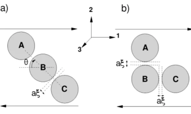
A triplet of spheres includes many-body interactions that are typically found in actual many-particle systems and can therefore be considered as a valuable validation for a lubrication correction method. Despite its simplicity and relevance, the case of three spheres in a shear flow has – as far as the authors know – no theoretical solutions nor reported simulation results. Two simple configurations are studied here and are sketched in Fig. 6. In each configuration, the triplet consists of equally-sized spheres suspended in a linear shear flow with shear rate ˙γ. The cubic domain size is 30a, with a grid resolution ∆=a/4.9 and a diffusional CFL number of 20. The non-dimensional separation distance ⇠ between spheres is set to 0.01. Sphere B is located at the center of the domain. In configuration (a), the orientation angle is ✓=30o(see Fig. 6).
As no theoretical solutions are available, reference numerical solutions for those two triplet configurations are first obtained using an alternative numerical method partly based on the commercial simulation software COMSOLr. The rigid motion is enforced by penalizing the strain tensor on the particle domain which leads to a generalized Stokes
Figure 6: Considered triplet configurations : (a) aligned configuration with orientation angle ✓=30o; (b) chair configuration. The non-dimensional
distance is ⇠=0.01
variational formulation. This basically corresponds to consider particle as a fluid with a very high viscosity. The method is implemented in the COMSOLrfinite element Stokes solver and more details on the penalty method used here may be found in [79, 80]. The COMSOLr mesh is fitted to the particles and refined on their surface. Grid convergence studies have been conducted so as to obtain a grid-independent solution. It is found that a grid spacing about 0.1a on particle surface and at least five grid points in the small 0.01a gap between particles are needed to resolve the lubrication flow properly. Preliminary computations with this penalty technique have been undertaken on two-sphere configurations and compared favorably with available theoretical solutions.
Comparisons between the COMSOLr solution (reference) and our computations are presented in Tab. 1 and Tab. 2 for the aligned and chair configurations. Translational and rotational velocities are non-dimensional using a ˙γ and ˙γ, respectively. As usual, subscripts (1, 2, 3) respectively denote the direction of velocity, velocity gradient and vorticity and superscripts (A, B, C) refer to the particles as depicted in Fig. 6. The average error is also specified in the bottom row of each table. Because particles are in the shear plane, velocities U3, ⌦1and ⌦2are equal to zero and are thus not given in the tables.
In both configurations, results are very encouraging especially in the aligned configuration where the average discrepancy is about 1 %. Results are not as excellent in the chair configuration but still remain acceptable. In this particular case, differences might possibly arise due to the pairwise approximation of lubrication forces. This approximation is well justified for short-range forces which is the case in the aligned configuration since interactions mostly come from a squeezing flow with a strong ⇠−1lubrication force. By contrast, the chair configuration rather induces a shearing flow between particles with a weaker log ⇠ singularity.
5.5. Sphere rolling down an inclined plane
The motion of a sphere rolling down an inclined planar surface due to gravity provides a convenient configuration for validating the coupling between lubrication and contact forces. A sphere of radius a, having microscopic asperities of uniform height hrug, is placed on a wall in a gravity field g = (g sin ✓,−g cos ✓, 0) to mimic an inclined plane with inclination angle ✓. Creeping flow conditions are assumed. Figure 7 presents the computed translational and rotational


![Figure 7: Non-dimensional translational U (diamonds) and rotational Ω (circles) velocities of a sphere moving down an inclined plane : computa- computa-tions (open symbols) and experimental results [81] (filled symbols)](https://thumb-eu.123doks.com/thumbv2/123doknet/13598762.423708/28.892.278.595.186.472/figure-dimensional-translational-diamonds-rotational-velocities-inclined-experimental.webp)