HAL Id: hal-01921194
https://hal.inria.fr/hal-01921194
Submitted on 13 Nov 2018
HAL is a multi-disciplinary open access
archive for the deposit and dissemination of
sci-entific research documents, whether they are
pub-lished or not. The documents may come from
teaching and research institutions in France or
L’archive ouverte pluridisciplinaire HAL, est
destinée au dépôt et à la diffusion de documents
scientifiques de niveau recherche, publiés ou non,
émanant des établissements d’enseignement et de
recherche français ou étrangers, des laboratoires
Reduction Semantics in Markovian Process Algebra
Mario Bravetti
To cite this version:
Mario Bravetti. Reduction Semantics in Markovian Process Algebra. Journal of Logical and Algebraic
Methods in Programming, Elsevier, 2018, 96, pp.41-64. �10.1016/j.jlamp.2018.01.002�. �hal-01921194�
Reduction Semantics in Markovian Process Algebra
Mario Bravetti
University of Bologna, Department of Computer Science and Engineering / FOCUS INRIA Mura Anteo Zamboni 7, 40126 Bologna, Italy
Abstract
Markovian process algebras allow for performance analysis by automatic genera-tion of Continuous Time Markov Chains. The inclusion of exponential distribu-tion rate informadistribu-tion in process algebra terms, however, causes non trivial issues to arise in the definition of their semantics. As a consequence, technical settings previously considered do not make it possible to base Markovian semantics on directly computing reductions between communicating processes: this would require the ability to readjust processes, i.e. a commutative and associative parallel operator and a congruence relation on terms enacting such properties. Semantics in reduction style is, however, often used for complex languages, due to its simplicity and conciseness. In this paper we introduce a new technique based on stochastic binders that allows us to define Markovian semantics in the presence of such a structural congruence. As application examples, we define the reduction semantics of Markovian versions of the π-calculus, considering both the cases of Markovian durations: being additional standalone prefixes (as in Interactive Markov Chains) and being, instead, associated to standard synchro-nizable actions, giving them a duration (as in Stochastic π-calculus). Notably, in the latter case, we obtain a “natural” Markovian semantics for π-calculus (CCS) parallel that preserves, for the first time, its associativity. In both cases we show our technique for defining reduction semantics to be correct with respect to the standard Markovian one (in labeled style) by providing Markovian extensions of the classical π-calculus Harmony theorem.
Keywords: Process Algebra, Structural Operational Semantics, Markov Chains
1. Introduction
The importance of considering probabilistic and timing aspects in system specification and analysis is widely recognized: first of all, the behavior of distributed systems and communication protocols often depends on probability and time; second, expressing duration of system activities makes it possible to estimate system performance. Markovian process algebras (see, e.g., [17, 1, 21, 16, 7, 4]) extend classical process algebras with probabilistic exponentially distributed time durations denoted by rates λ (positive real numbers), where λ is the parameter of an exponential distribution. Defining an operational
semantics for a Markovian process algebra makes it possible to derive Continuous Time Markov Chains from system specifications, which can then be analyzed for performance. Essentially this requires generating, from rates λ expressed syntactically in the prefixes of the process algebra, transitions labeled by rates. Markovian process algebras in the literature have been defined in technical settings where it is not possible to compute their transitions by readjusting par-allel processes, i.e. to represent their evolution by (not action labeled) reduction transitions (see, e.g., the reduction semantics of π-calculus [22, 19]). This is due to limitations in existing approaches to Markovian operational semantics that make them not compatible with a structural congruence relation. In reduction semantics such a relation is endowed with commutative and associative laws of parallel that allow communicating processes to get syntactically adjacent to each other in order to directly produce reduction transitions. The incompatibility arises from the techniques used for managing multiplicity of rate transitions: a Markovian semantics, in order to be correct must express multiplicity of several identical transitions, that is transitions with the same rate λ and source and tar-get terms. Process algebras enriching prefixes with Markovian rates λ previously introduced in the literature use, instead, semantical definitions in the labeled operational semantics style: transitions are labeled with actions (representing potential of communication) and actual communications are produced by match-ing transitions of parallel processes accordmatch-ing to their action labels. Reduction semantics is, however, widely used, since, due to its simplicity and conciseness, it is convenient for defining semantics of complex languages, see, e.g., [18].
Moreover, for Markovian process algebras where CCS/π-calculus parallel is used and both output and input actions are quantified by rates/weights, existing approaches in the literature (e.g. stochastic π-calculus of [21]) do not even guarantee associativity of parallel. That is in general, unless specific restrictions on the structure of terms are assumed (see [9]), different rates are obtained for outgoing transitions of terms (P |Q)|R and P |(Q|R).
In this paper we present a technique that allows us, for the first time, to develop semantics for Markovian process algebra in reduction style, i.e., where transitions are not labeled with actions and are directly produced by readjusting the structure of terms via a structural congruence relation. This opens the new possibility to include rates λ in actions of complex languages like that of [18] with no need to completely change the semantics from reduction to labeled style and without losing important properties like associativity of parallel. Notably, for the above mentioned case of Markovian process algebras where both output and input actions are quantified by rates/weights, our reduction semantics is the first Markovian one preserving associativity of CCS/π-calculus parallel.
More precisely, we consider stochastic versions of the π-calculus, encompassing both the case of rates being additional standalone prefixes and rates being, instead, attached to standard action prefixes. In the former case, Markovian delay prefixes (λ) are expressed separately from standard actions (that are unmodified) as in the Interactive Markov Chains approach of [16]. In the latter case, we instead decorate π-calculus output and τ prefixes with a λ rate, denoting Markovian actions. We consider two variants for this case. In the first variant
input prefixes are not explicitly quantified (they are syntactically unmodified) and τ resulting from the synchronization of a λ decorated output on channel “a” and an input on “a” simply has rate λ: this corresponds to multiplying λ by the number of possible synchronizations over “a”, similarly to what is done in the context of biochemistry, see e.g. [8]. In the second variant input prefixes are, instead, endowed with weights w, i.e. numbers establishing the probability to choose an input on channel “a” given that “a” is the channel of the selected output: this corresponds to subdividing the output rate λ among the possible “a” synchronizing inputs according to their weights, as done in Stochastic π-calculus [21] by taking inputs to have (weight equipped) unspecified rates [17, 21].
In all above cases, we first define the semantics of the Markovian calculus in labeled operational semantics style (we use the early semantics of the π-calculus) using the classical approach of [14, 21] to deal with multiplicity of identical transitions. We then apply our technique, which, as we will see, is based on the use of so-called stochastic names and stochastic binders (for both rates and weights) to provide a reduction semantics for the same process algebra.
We finally show our approach to correctly calculate rates (manage their multiplicity) by means of a theorem similar to the Harmony Lemma in [22, 19], that is: stochastic reductions of reduction semantics are in correspondence with Markovian (τ ) transitions of the labeled operational semantics and, thus, the underlying Markov chains. We show such a theorem to hold both for Markovian delays and actions, but not for the variant with input weights: this is related to the fact that parallel of Stochastic π-calculus [21] is not associative. If, e.g., in [21] we consider P |(P0|P00) with P = x<y>
3.Q, P0= x(z)4.Q0 and P00= x(z0)8.Q00 (we
represent a prefix rate as a subscript), we get two distinguished τ transitions with rates 1 and 2. That is, rate 3 of the output multiplied by the probability to choose, inside P0|P00 (the subterm to the right of the parallel where synchronization
happens): either input x(z)4, i.e. 4/12 (the rate of the input divided by the
total rate of inputs on x in P0|P00); or input x(z0)
8 in P0|P00, i.e. 8/12 (similarly
calculated). Rates of inputs are therefore treated as weights, according to which the output rate 3 is distributed. If, instead, we consider (P |P0)|P00 [21] yields two distinguished τ transitions with the same rate 3. That is, rate 3 of the output multiplied by the probability: to choose x(z)4 inside P0, i.e. 4/4 (the
rate of the input divided by the total rate of inputs on x in P0); and to choose
input x(z0)
8 inside P00, i.e. 8/8.1
As shown also in [12] non associativity of parallel comes from the fact that [21] calculates rates, upon synchronization, in a way that strictly depends on a fixed structure for parallel operators in the term (independently of the particular labeled semantic technique used to deal with rates - [9], [12] or the original [21]):
1In this example rates of inputs are treated as weights because, for all parallel operators P1|P2considered, the total rate of outputs on x in P1is smaller than the total rate of input on x in P2 (see [21]): the same is obtained by taking rates of inputs as (weight equipped) unspecified rates of [17, 21].
the rate of a synchronization on channel x performable by P1| P2, depends on
the total rate of input/output transitions on x performable by P1 and P2, called
apparent rate in [17, 21]. By using our reduction semantics technique, instead, the calculation of the total weight is not based on such a fixed structure, but it is the sum of weights of all synchronizable input actions (independently of how parallel is associated), hence parallel is dealt with in an associative way: in the example above we consider for the calculation of the total weight all input actions synchronizable with x<y>3, thus getting two reductions with rates 1
and 2 independently on how parallel is associated. This is natural in the context of π-calculus (or CCS) parallel P1|P2 in which, differently from CSP parallel
(originally used when Markovian semantics and apparent rate was defined [17]), an action of P1that can be synchronized with one of P2can also be synchronized
with one performed by an outer parallel process.
1.1. The Problem of Dealing with Structural Congruence
We now explain why, due to the technique used for expressing multiplicity of identical transitions, previous approaches for extending process algebras with Markovian durations are not compatible with the use of a structural congruence, as needed in reduction semantics.
Among techniques previously considered, the simplest one (see [17]) is count-ing the number of different possible inferences of the same transition in order to determine its multiplicity. However this can be done only for semantic definitions that do not generate transitions by means of a structural congruence relation ≡ on terms, that is via the classical operational rule of closure w.r.t. ≡ that makes it possible to infer a transition P −→ Qα 0 from Q α
−→ Q0 whenever P ≡ Q. This
is because, the presence of such a rule causes the same transition to be inferred in a number of ways even in the case of just one occurrence of a Markovian delay; e.g., considering P just being a single Markovian delay and the common congruence law P ≡ P |0, such a number would even be infinite.
Another similar way used in the literature (see, e.g., [14, 21]) to deal with Markovian transition multiplicity is to explicitly introduce a mechanism to differ-ently identify multiple executions of identical Markovian delays by introducing some kind of identifier that typically expresses syntactic position of the delay in the term (e.g. it is called a “location” in the case of the position with respect to the parallel operator) and whose syntax is dependent on the operators used in the language. Again, since Markovian transitions are, roughly, identified by indicating the path (left/right at every node) in the syntax tree of the term, this solution is not compatible with using a structural congruence relation with commutative and associative laws that readjusts term structure at need during inference. As already said, we will use this approach to express the labeled operational semantics of the Markovian process algebras that we consider in this paper and for comparison with our reduction semantics.
Finally, techniques exploiting the representation of Markovian transitions collectively as a distribution over a target state space (a traditional approach in the context of probabilistic transition systems, see Giry functor [13] and its generalizations, e.g., [23, 11, 24]) have been used in [9] and in [12] for any
Markovian process algebra whose operational rules satisfy a Markovian extension of the GSOS rule format. These techniques are crucially based on collectively inferring Markovian transitions performable at a certain syntactic level (e.g. in P | Q) from transitions performable at lower levels (e.g. by P and by Q). Therefore, they are, again, not compatible with using structural congruence ≡ (with commutative and associative laws) for generating transitions, as caused by the operational rule of closure w.r.t. ≡ mentioned above. Formally, such a rule is indeed not in the GSOS format of [12], hence the approach of [12] cannot be used in its presence. It is, however, a fundamental rule in reduction semantics. Conceptually, the reason for incompatibility is that, due to this rule, different transitions may need different structural readjustments to be inferred: e.g. given term P |(Q|R) it can be that it needs to be readjusted into (P |Q)|R to infer a Markovian reduction due to P communicating with Q and to (P |R)|Q to infer a Markovian reduction due to P communicating with R. So we cannot fix a stratification of transition inference, that is first collectively inferring all transitions of (Q|R) and then use them to infer all transitions of P |(Q|R): for each Markovian reduction of P |(Q|R) it must be possible to individually perform a different readjustment of parallel.
1.2. Main Idea
In this paper we present a technique for defining semantics of a Markovian process algebra in the presence of structural congruence. This allows us to define Markovian semantics in reduction style. As already mentioned, our technique is applicable for Markovian extensions of process algebra obtained: either by simply adding Markovian (λ) delay prefixes or by decorating existing action prefixes with λ. Our technique is also compatible with standard unfolding of recursion made by structural congruence: the possibility of expressive cycling behavior via a recursion operator is fundamental for steady state based performance analysis. Moreover, our technique is such that the inclusion of rates λ in process algebra prefixes does not cause a significant modification of process algebra semantics, in that most of the burden is concentrated in few additional rules which are independent of the particular operators used by the algebra. More precisely, we do not have to introduce an explicit (operator dependent) mechanism to distinguish multiple occurrences of actions as in [14, 21], or to intervene in the semantics of every operator as in [9] or to separately define, by induction on term syntax, how rate distributions are calculated using (total) rate information attached to rules as in [12] (which also does not cope with recursion).
The idea is to introduce stochastic names (that can be seen as names for stochastic variables) and stochastic binders (binders for such names). Stochastic names are used in process algebra prefixes and rates λ are assigned to them by the corresponding stochastic binder. In essence (a set of) stochastic binders act as a (probabilistic/stochastic) scheduler: they use names attached to prefixes to collectively quantify them. In this way, assuming that all prefixes are associated with a different stochastic name, rate values replace stochastic names upon binding and multiplicity is correctly taken into account because prefixes with the same rates are anyhow distinguished by having different stochastic names.
But how to guarantee that prefixes are given different stochastic names? The idea is to consider a specification language where rates λ are in prefixes and then to turn them (by laws of structural congruence) into stochastic names that are immediately bound by a stochastic binder assigning the rate λ. Then, with the usual rules of binder extrusion, we impose that, before binders can be evaluated, they must be all lifted to the outermost syntactic level by structural congruence. As a consequence we have the guarantee (due to the requirement of α-conversion related to binder extrusion) that every prefix is assigned a distinguished stochastic name. Note that recursion is dealt with in the correct way as well, because, as we will see, recursions need to be unfolded in order to perform the lift of the binders.
1.3. Paper Outline
The paper is structured as follows. Section 2 presents the extension of π-calculus with Markovian delays (λ) and its labeled operational semantics according to the classical technique of [21]. Section 3 introduces our technique, uses it for defining semantics in reduction style of the algebra of Section 2 and shows the obtained semantics to be correct w.r.t. the labeled one via an Harmony theorem. Section 4 considers the π-calculus extension with Markovian actions in both versions (with and without weights) and, for each of them, presents: its labeled semantics according to the classical technique of [21], our semantics in reduction style and comparison results via a second Harmony theorem. Finally, Section 5 concludes the paper by further discussing related work. Appendices A and B include proofs of the more involved results presented in Section 3 and 4, respectively. Initial work was carried out in the technical report [2].
2. Classical Approach for Markovian Delays
We consider the π-calculus with constant definitions (as in [20]) extended with Markovian delay prefixes, following the Interactive Markov Chain approach of [16]. Markovian delays are thus simply represented by (λ) prefixes, where λ is the rate of an exponential distribution. As usual in the context of Markovian process algebra, see, e.g., [21]: we consider recursion by constant definitions (as done for the standard π-calculus, e.g., in [20]) and not by a bang operator; and we assume recursion to be (weakly) guarded. In this way we avoid terms like A= A|(λ).P for which we would not get a finite cumulative rate for the∆ outgoing Markovian transitions of A.
Let x, y, . . . range over the set X of channel names and λ range over the set R
I + of rate values, representing rates of exponential distributions. Definition 2.1. We take P to be the set of terms P, Q, . . . generated by
P ::= M | P |P0| (νx)P | A(x1, . . . , xn)
M ::= 0 | α.P | M + M0
We abbreviate x1, . . . , xn with ˜x and we assume a given set of constant
definitions A(˜x)= P such that the following is satisfied. We can, by starting∆ from P and by performing a finite number of successive substitutions of constants B(˜y) for their defining term Q{˜y/˜x} (assuming B(˜x)= Q), obtain a term P∆ 0 where every constant occurs in P0 in the scope of a prefix operator (A is weakly guarded defined, see [20]).
Concerning the labeled operational semantics we consider the early semantics of the π-calculus (see, e.g., [22]) and, concerning Markovian delays, the classical approach of [21], i.e. we use an explicit (operator dependent) mechanism to distinguish multiple occurrences.
Operational semantics is thus defined by the following labeled transition system. We assume η to range over its labels and transitions be of two kinds:
• The classical π-calculus early semantics labeled transitions, defined in Table 1. We assume: symmetric rules to be also included, as usual; the meaning of labels and the definition of functions n (names), bn (bound names) and fn (free names) to be the standard one, see, e.g., [22]; and µ to range over the set of standard labels, i.e. xy, x(y), xy or τ labels. • Markovian transitions, defined via the additional rules in Table 2, that
are labeled with pairs “λ, id” where: λ is the rate of the Markovian delay being executed and id is a unique identifier. An identifier id is a string over the alphabet {+0, +1, |0, |1} ending with an additional “•” and represents
the syntactic position of the delay in the syntax tree of the term (once, constant replacement is applied if needed), i.e. the path in the tree. Notice that η ranges over both standard labels µ and labels “λ, id” of Markovian transitions, which are defined by the rules in Table 2 and the relevant rules of Table 1.
Example 2.1. Consider P = (3).P0+(3).P0. We have that P performs transi-tions:
P−−−3, +−→ P0• 0 P−−−3, +−→ P1• 0
Notice that, thanks to the use of identifiers, we get two transitions for P (without them we would have got just one) and we correctly have that the total rate of transiting from P to P0 is 6.
Consider now P | Q, with P as above. It performs (P originated) transitions: P | Q 3, |−−−0−→+0• P0| Q
P | Q
3, |0+1•
−−−−→ P0| Q
Again, thanks to the use of identifiers, we correctly have that the obtained overall rate of (P originated) transitions from P | Q to P0|Q is 6.
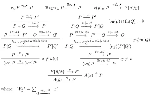
τ.P −→ Pτ x<y>.P −→ Pxy x(y).P xy 0 −→ P {y0/y} P −→ Pµ 0 P + Q−→ Pµ 0 P −→ Pµ 0 P |Q−→ Pµ 0|Q bn(µ) ∩ fn(Q) = ∅ P −→ Pxy 0 Q−→ Qxy 0 P |Q−→ Pτ 0|Q0 P −→ Px(y) 0 Q−→ Qxy 0 P |Q−→ (νy)(Pτ 0|Q0) y /∈ fn(Q) P −→ Pη 0 (νx)P −→ (νx)Pη 0 x /∈ n(η) P −→ Pxy 0 (νy)P x(y)−→ P0 y 6= x P {˜y/˜x}−→ Pη 0 A(˜y)−→ Pη 0 A(˜x) ∆ = P
Table 1: Standard Rules (Symmetric Rules Omitted)
(λ).P −→ Pλ,• P −→ Pλ,id 0 P + Qλ,+−→ P0id 0 Q−→ Qλ,id 0 P + Qλ,+−→ Q1id 0 P −→ Pλ,id 0 P |Qλ,|−→ P0id 0|Q Q−→ Qλ,id 0 P |Qλ,|−→ P |Q1id 0
Table 2: Identified Markovian Transitions
The labeled transition system arising from the semantics of a term P has states with both outgoing Markovian and standard transitions: it has to be interpreted as an Interactive Markov Chain of [16], with τ transitions being instantaneously executed and other π-calculus labeled transitions representing potential for execution. In particular Markovian transitions performable in states that also have outgoing τ transitions are considered to be pre-empted (so-called maximal progress assumption) and a system is considered to be complete if it cannot undergo further communication with the environment, i.e. it can perform only τ and Markovian transitions.
This is expressed by the notion of Markovian Bisimulation considered in [16] and that we also report here. We first define the total rate γ(P, P0) of transiting from state P to P0 via Markovian transitions as
γ(P, P0) = X
P λ,id−→ P0
λ
to sets of states in the usual way:
γ(P, Set) = X
P0∈Set
γ(P, P0)
We can now consider the Markovian bisimulation as in [16] (see [16] for weak bisimulation definition abstracting, when possible, from τ transitions).
Definition 2.2. An equivalence relation B on P is a strong bisimulation iff P B Q implies for all µ and all equivalence classes C of B
• P −→ Pµ 0 implies Q−→ Qµ 0 for some Q0 with P0BQ0
• P 6−→ implies γ(P, C) = γ(Q, C)τ
Two processes P and Q are strongly bisimilar if (P, Q) is contained in some strong bisimulation B.
3. Reduction Semantics for Markovian Delays
We now use our technique based on symbolic representation of rates via stochastic names and binders to give a semantics in reduction style for the Markovian π-calculus of Section 2.
3.1. Stochastic Names and Stochastic Binders
We extend the syntax of terms P, Q, . . . by adding stochastic names and stochastic binders. We use q, q0, . . . ∈ QN to range over stochastic names, i.e. names used to express symbolically stochastic information for delays. Moreover θ, θ0, . . . ranges over channel names and stochastic names, i.e. the set X ∪ QN . Definition 3.1. We take Pext to be the set of terms P, Q, . . . generated by
extending the syntax of P terms in Definition 2.1 as follows: P ::= . . . | (νq → λ)P
α ::= . . . | (q)
The idea is that we can now represent (λ) delays by means of a stochastic name q that can be seen as the name of a stochastic variable. More precisely a delay (λ) can be equivalently represented by (q) in the scope of a stochastic binder (νq → λ) that associates rate λ to the stochastic name q (i.e. the binder “quantifies” q). In the following we use (νx → ε) to stand for (νx), i.e. the standard π-calculus binder, which does not associate any “quantification” to x. This will allow us to write (νθ → bλ) to stand for any binder (stochastic or classical) by assuming bλ, bλ0to range over RI +∪ {ε}.
Notice that we will use Pext terms over the extended syntax to define the
semantics of P terms in reduction style. As we will see, for every state of the semantics we will always have a congruent term which belongs to P. The definition of structural congruence follows.
(νθ →bλ)P | Q ≡ (νθ →bλ)(P |Q) if θ /∈ fn(Q) (νθ →bλ)(νθ0→ bλ0)P ≡ (νθ0→ bλ0)(νθ →bλ)P if θ 6= θ0 (νθ →bλ)0 ≡ 0 (M1+ M2) + M3 ≡ M1+ (M2+ M3) M + N ≡ N + M M + 0 ≡ M (P1|P2)|P3 ≡ P1|(P2|P3) P |Q ≡ Q|P P |0 ≡ P
A(˜y) ≡ P {˜y/˜x} if A(˜x)= P∆
Table 3: Standard Structural Congruence Laws (with quantified binders)
We consider a structural congruence relation over processes in Pextdefined
as usual by a set of laws. We consider the standard laws in Table 3 (where we just add the possible presence of quantification in binders) and, in addition, the following law:
(λ).P + M ≡ (νq → λ)( (q).P + M ) if q /∈ fn(M, P )
As usual, alpha renaming inside processes, for any name θ and its binder (νθ →bλ) is assumed. Concerning the use of parentheses when writing terms in the laws above and in the following, we assume binding to take precedence over parallel and prefix to take precedence over sum.
3.2. Operational Semantics
We now define the semantics of the process algebra of Definition 3.1 in reduc-tion style. As we will see besides standard reducreduc-tion transireduc-tions (defined with standard rules), we have two other kinds of transitions representing stochastic execution. Transitions labeled with a stochastic (delay) name, which are treated similarly to standard reduction transitions, and stochastic transitions, which are generated when a stochastic binder is applied at the top level. The latter lead from a term to a rate distribution over terms.
We consider rate distributions σ, in the style of the probabilistic model of [23] (also used by [9] in the context of Markovian rates), describing how a state can
be reached from another one by performing a Markovian transition.
Definition 3.2. A rate distribution σ over a countable set S is a non-empty finite multiset over RI +× S, i.e. a multiset of pairs (λ, e), with λ ∈ RI + and e ∈ S. We use RDist(S) to denote the set of rate distributions over S.
Due to use of the structural congruence relation, it will be convenient to use rate distributions σ over congruence classes of terms, i.e. σ ∈ RDist(Pext/ ≡),
instead of single terms (as, e.g., done in [9]).
(q).P + M −→ Pq τ.P + M −→ P x<y>.P + M | x(z).Q + N −→ P | Q{y/z} P −→ Pbq 0 P |Q b−→ Pq 0|Q P −→ Pbq 0 (νθ →bλ)P −→ (νθ →bbq λ)P0 θ 6=qb P ≡ Q Q b−→ Qq 0 Q0≡ P0 P −→ Pbq 0
Table 4: Standard Rules for Reductions and Symbolically Quantified Transitions
• Standard reductions [19], denoted by P −→ P0, that represent action
execution.
• Transitions similar to the standard reductions of [19] that represent delay executions and just differ from reductions in that they are additionally labeled with the name q associated with the delay: their quantification is symbolic in that the name of the delay is included and not the actual rate. They are denoted by P −→ Pq 0.
• Stochastic transitions leading from a term to a rate distribution over congruence classes of terms. They are denoted by P −→ σ, where σ ∈ RDist(Pext/ ≡).
The first two relations are collectively defined as the smallest subset of Pext× (QN ∪ {ε}) × Pext (where ε labeled reductions represent the standard
ones of [19], i.e.−→ stands for −→ ) satisfying the operational rules in Table 4.ε We assumebq, used in Table 4 to denote transition labels, to range over stochastic names q and ε, i.e.bq ∈ QN ∪ {ε}. Notice that, with respect to the standard ones of [19], the rules in Table 4 only differ in including a rule for (q) prefix and in considering names q ∈ QN as possible reduction labels (and rates λ possibly associated to binders).
Stochastic P −→ σ transitions are defined as the smallest subset of Pext×
RDist(Pext/ ≡) satisfying the operational rules in Table 5, where we assume
(νq → λ)σ = {| (λ0, [(νq → λ)P ]≡) | (λ0, [P ]≡) ∈ σ |}.2 Notice that, even if (Sto2)
rule includes a negative premise, the operational semantics is well-defined in that the inference of transitions can be stratified (see, e.g., [15]).
The idea behind the semantics is that, since in Table 5 we do not have rules for other operators besides stochastic binders, in order for a stochastic P −→ σ transition to be generated, term P must be rearranged by structural congruence in such a way that all its stochastic binders (those actually binding a (q) delay prefix) are the outermost operators, i.e. they must be all extruded up to the top
(Sto1) P −→ σ P q −→ P0 (νq → λ)P −→ (νq → λ)σ ∪ {| (λ, [(νq → λ)P0]≡) |} (Sto2) 6 ∃ σ : P −→ σ P q −→ P0 (νq → λ)P −→ {| (λ, [(νq → λ)P0]≡) |} (StoCong) P ≡ Q Q −→ σ P −→ σ
Table 5: Rules for Stochastic Transitions
level. For instance, considering P = (νq → λ)( (q) | (νq0 → λ0)(q0) ), one could
think that a stochastic transition for P , erroneously containing the λ rate only, could be inferred by the rules, i.e. a “partial” stochastic transition. On the contrary, this cannot happen because (q) | (νq0 → λ0)(q0) does not satisfy the
negative premise of rule (Sto2): the reason being that (q) | (νq0 → λ0)(q0) can
be rearranged to (νq0→ λ0)( (q) | (q0) ). Moreover, since we consider stochastic
P −→ σ transitions only for terms P ∈ Pext such that there exists P0 ∈ P with
P ≡ P0 (as we will see, all terms P that are reachable by transitions of the
operational semantics from an initial term in P are in this form), we have that multiple outgoing stochastic transitions for the same P cannot be produced. This is a consequence of the fact that in such terms P each stochastic binder binds at most one (q) prefix (and of the fact that the “partial” stochastic transitions mentioned above cannot be produced). Summing up, we have that for such terms P , either no P −→ σ transiton is generated or a single P −→ σ transition is generated. In the latter case it correctly evaluates the multiset of Markovian transitions leaving a state on the basis of symbolic delay transitions, each of which (since all stochastic binders must have been extruded up to the outermost level) is guaranteed to have a different name. All these facts, for which we gave here just an informal intuition, will be proved formally in the following (Propositions 3.1, 3.2, 3.3 and the Harmony Theorem 3.1).
Example 3.1. Consider P = (5).A|(5).A and A= (5).A. We have that, ac-∆
cording to the standard labeled semantics presented in Section 2, P performs transitions: P 5,|0• −−−−→ A | (5).A P 5,|1• −−−−→ (5).A | A
Let us now apply our reduction semantics to P . We have that P ≡ (νq → 5)(q).A | (νq → 5)(q).A ≡
(νq → 5)(νq0 → 5)( (q).A|(q0).A )
thus P performs the stochastic transition
that is a multiset including two instances of the same pair.
This is because, after applying (Sto1) and (Sto2), we get P −→ σ0 with σ0= {| (5, [(νq → 5)(νq0 → 5)(A|(q0).A)]≡), (5, [(νq → 5)(νq0 → 5)((q).A|A)]≡) |}
= {| (5, [(νq0→ 5)(A|(q0).A)]≡), (5, [(νq → 5)((q).A|A)]≡) |}
= {| (5, [A|(5).A]≡), (5, [(5).A|A]≡) |} = σ
The example shows that, at every (stochastic) transition, stochastic binders are moved:
• first inside-out (from prefixes to the top-level) to make it possible to apply (Sto1) and (Sto2) rules;
• then outside-in (back, so to be eliminated or become prefixes again) in order to obtain again a representative in P for each of the reached congruence classes.
This shows that, differently from other uses of “unique names” in the literature (as e.g. for expressing ST semantics [6]), where the purpose of the generated names is to uniquely identify elements across multiple subsequent transitions, here names are generated for the sole purpose of uniquely identifying single transitions and can be forgotten after the transition itself is performed.
The transition system of terms can be represented in a finitary way by taking states to be congruence classes [P ]≡∈ Pext/ ≡ (recall that, due to standard laws
like P |0 ≡ P , every term has an infinite number of congruent terms). This will be important when deriving, as done in Section 2 for the labeled operational semantics, the underlying Interactive Markov Chain.
Definition 3.3. Let P, P0 ∈ Pext. We define [P ]≡ b q
−→ [P0]≡whenever P b q
−→ P0.
Let P ∈ Pext and σ ∈ RDist(Pext/ ≡). We define [P ]≡ −→ σ whenever
P −→ σ.
The above is well-defined because congruent terms P have the same outgoing transitions (rule of closure w.r.t. congruence in each of Tables 4 and 5).
Notice that, it would have also been possible to define directly transitions on equivalence classes, instead of resorting to Definition 3.3, by putting equivalence classes inside rules, e.g. for parallel
[P ]≡ b q −→ [P0] ≡ [P |Q]≡ b q −→ [P0|Q] ≡
This would have also made the two rules of closure w.r.t. congruence in each of Tables 4 and 5 superfluous (working directly with classes yields the same effect). For the sake of clarity and readability, we preferred however to stick to the more standard approach of defining semantics via rules of closure, which also avoids burdening all other rules with the equivalence class notation around terms.
3.3. Properties and Results
Let us now analyze properties of (outgoing) transitions of terms P ∈ P, that is, terms belonging to the non-extended syntax of Definition 2.1. Notice that, since congruent terms have the same outgoing transitions, such properties obviously hold also for terms P ∈ Pextsuch that P ≡ P0 for some P0∈ P.
The following proposition says that terms P of the non-extended syntax can just perform standard reductions and stochastic transitions. This means that, for such terms P , the −→ transitions are used only during inference ofq stochastic transitions.
Proposition 3.1. Let P ∈ P. There is no P0 ∈ Pext, q ∈ QN such that
P −→ Pq 0.
Proof. A direct consequence of the fact that for any Q ≡ P , with P ∈ P, we have that, due to the laws of ≡, all delay prefixes (q) occurring in Q are bound (rules for binders do not allow transitions labeled with the bound name to be
inferred). 2
We now present a crucial property, which we informally discussed in Sec-tion 3.2, of our reducSec-tion semantics that shows that the semantics of stochastic transitions is well-defined: if a P ∈ P term has an outgoing stochastic transition P −→ σ then it is unique. Notice that, besides the intuitive observations we already made in Section 3.2, this also entails proving that, no matter the order in which we choose to solve stochastic binders, we get a stochastic transition with the same σ (this is one of the sources of the complexity of the proof).
Proposition 3.2. Let P ∈ P and P −→ σ. We have P −→ σ0 implies σ = σ0.
Proof. The proof, reported in Appendix A, essentially shows that, supposing n to be the number of Markovian delays “immediately performable” by P and q1,
. . . , qn any set of distinguished names, there exists P0 such that P ≡ (νq1→
λ1) . . . (νqn → λn)P0 and ∀h, 1 ≤ h ≤ n. P0 qh
−→ P0
h. Moreover for any such P0
we have:
σ = σ0= {| (λ1, [(νq1→ λ1) . . . (νqn→ λn)P10]≡) |} ∪ . . . ∪
{| (λn, [(νq1→ λ1) . . . (νqn→ λn)Pn0]≡) |}
2 Finally we show that for any P0 ∈ Pext that is reachable by performing
transitions from a term P ∈ P (i.e. a term belonging to the non-extended syntax) it is always possible to find a term P00∈ P that is congruent to P0.
Proposition 3.3. Let P ∈ P and P0 ∈ Pext such that: P −→ P0 or P −→ σ ∧
∃λ : (λ, [P0]
Proof. For any Q ≡ P with P ∈ P we have: all delay prefixes (q) occurring in Q are bound and every stochastic binder can bind at most a single delay prefix (q). It is easy to verify that this property is preserved by reductions Q −→ Q0 or transitions Q −→ σ for which ∃λ such that (λ, [Q0]≡) ∈ σ, i.e. for any such Q0
the same property holds true. For instance performing the σ transition causes the corresponding stochastic binder to not bind any delay prefix in the target state. Any Q0 satisfying the property above can be shown to be congruent to a term of P by just removing stochastic binders not binding any delay prefix and by turning stochastic binder binding a single delay prefix (q) into a Markovian
delay prefix. 2
A consequence of the above propositions and of Definition 3.3 is that, given P ∈ P, we can represent the semantics of P as a transition system whose initial state is [P ]≡ and, in general, states (congruence classes reachable from [P ]≡) are
[P0]≡ such that P0∈ P: such classes always have a representative in P.
Concerning the underlying Interactive Markov Chain, we have:
• the rate γ([P ]≡, [P0]≡) of transiting from state [P ]≡ to state [P0]≡ is:
P
(λ,[P0]≡)∈σλ · µσ(λ, [P0]≡) if [P ]≡ −→ σ for some σ; 0 otherwise3
• τ transitions of the Interactive Markov Chain are standard reductions. The above also provides a definition of bisimulation over states of P ∈ P by applying it to Definition 2.2 (and to other equivalences in [16]). Obviously, w.r.t. the Interactive Markov Chain obtained by labeled operational semantics, reduction semantics of a term P yields a closed system interpretation, i.e. as if all (free) actions of P were bound at the top level. Therefore the obtained Interactive Markov Chain is just labeled with τ actions as for all Interactive Markov Chains corresponding to complete systems, which are commonly the ones to be analyzed for performance.
We now formalize this correspondence. This has been done for the π-calculus, see, e.g., Harmony Lemma in [22] or [19]. Here we extend this result to Markovian delays, thus also showing correctness of the stochastic binder idea: in particular that the semantics of stochastic transitions correctly deals with rate multiplicity of identical transitions and that all delays are actually accounted for when calculating the stochastic transition of a term (see discussion about “partial” stochastic transitions in Section 3.2).
Theorem 3.1 (Harmony). Let P ∈ P. We have:
• P −→ P0 iff P τ
−→ ≡ P0
• P −→ σ for some σ iff P −→ Pλ,id 0 for some λ, id and P0. Moreover, when
3We assume an empty sum to yield 0. Given a multiset m, µm(e) denotes the number of occurrences of element e in m.
both hold, we have that ∀P0 ∈ P X (λ,[P0] ≡)∈σ λ · µσ(λ, [P0]≡) = X Pλ,id−→ ≡P0 λ
Proof. The proof, reported in Appendix A is based on that of Proposition 3.2: in particular on the structure, we previously presented, of the unique σ (if any) such that P −→ σ and on the following observations. Assume q1, . . . ,
qn to be any set of distinguished names. Given Q including unique
occur-rences of prefixes (q1), . . . , (qn) in its “immediate behaviour” and such that
P ≡ Q{λi/qi | 1 ≤ i ≤ n}, we have P ≡ (νq1 → λ1) . . . (νqn → λn)Q and
∀h, 1 ≤ h ≤ n. Q qh
−→ Q0
h. Moreover, for each index h, with 1 ≤ i ≤ h, and
Q00h such that Q{λi/qi | 1 ≤ i ≤ n} λh,idh
−→ Q00h there exists Ph0, with Ph0 ≡ Q00h, such that P λh,idh
−→ P0
h; and vice versa. The proof shows that both sides of the
theorem equation, thus, yieldP
h∈Iλh, with I being the set of indexes h such
that Q00h≡ P0. 2
4. Markovian Actions
We now consider the two variants, we discussed in the introduction, extending π-calculus with rates attached to actions: for each of them we present a labeled operational semantics using the classical approach of [21] and extensions of our technique based on stochastic binders and stochastic names to produce a reduction semantics. With respect to Markovian delays, having rates attached to actions complicates significantly the problem of developing a (correct) semantics in that Markovian transitions are no longer simply generated from standalone prefixes, but are produced by synchronization of an output and an input (under a specific rule for calculating the rate of the τ transition obtained by synchroniza-tion). In both variants that we consider output and τ prefixes are endowed with a rate: their difference stems from the way inputs are dealt with (and in how the synchronization rule mentioned above is defined). In the simpler variant input prefixes are not explicitly quantified, while in the other one they are endowed with a weight. Similarly to what we did for Markovian delays, for both versions we will: study the properties of the presented reduction semantics, show how to derive the underlying Markov Chain, and compare them with the standard labeled semantics.
4.1. Syntax
In π-calculus with Markovian Actions we extend the syntax of output x<y> and τ prefixes by attaching a Markovian rate λ to them: for the sake of simplicity we just represent it as a subscript, i.e. x<y>λand τλ. Concerning input prefixes,
• non-quantified inputs, in which input prefixes are not explicitly quantified (their syntax is unmodified w.r.t. π-calculus). The idea is that the τ transition resulting from the synchronization of a λ-decorated output on channel “a” and an input on “a” simply has rate λ: this corresponds to multiplying λ by the number of possible synchronizations over “a”, similarly to what is done in the context of biochemistry, see e.g. [8]. • weighted inputs, in which input prefixes are endowed with weights w ∈ RI +,
i.e. numbers establishing the probability to choose an input on channel “a” given that “a” is the channel of the selected output, as for the Stochastic π-calculus [21] with inputs having (weight equipped) unspecified rates [17, 21]. We take the two above versions of π-calculus with Markovian actions to have the same syntax as π-calculus with Markovian delays (Definition 2.1), apart from redefinition of prefixes α. We denote: with Pra (pointing out that now we have rates λ attached to actions, instead of having them in separate prefixes) the set of terms of π-calculus with Markovian actions and non-quantified inputs; with Pwra (pointing out that we additionally have weights) the set of terms of π-calculus with Markovian actions and weighted inputs.
Definition 4.1. We take Pra to be the set of terms P, Q, . . . generated by
P ::= M | P |P0| (νx)P | A(x1, . . . , xn)
M ::= 0 | α.P | M + M0
α ::= x<y>λ| x(y) | τλ
We take Pwra to be the set of terms P, Q, . . . generated by the same syntax, where
in the definition of prefixes α we consider inputs x(y)w, instead of x(y).
In the following we use γ ∈ RI + to range over both rates λ and weights w.
4.2. Classical Approach
We now define the labeled operational semantics of the two considered versions of π-calculus with Markovian Actions, using the classical approach based on (operator dependent) identifiers.
4.2.1. Non-quantified Inputs
With respect to Section 2, we now have a single (combined) kind of transition, that is Markovian and labeled transitions P −→ Pυ,id 0, where υ is any of xyλ, x(y)λ,
xy or τλand id is the identifier used to distinguish identical transitions (in order
to correctly account for their multiplicity). The identification based approach of Section 2 must, thus, be now extended to also represent Markovian transitions obtained by synchronization. We do this by enriching the syntax of identifiers id with the construct h|0id1, |1id2i, where id1, id2 are themselves identifiers,
see [21]. Thus the syntax of identifiers is now:
τλ.P τλ,• −→ P x<y>λ.P xyλ,• −−−−→ P x(y).P xy 0,• −−−−→ P {y0/y} P −→ Pυ,id 0 P + Q −−−υ,+−→ P0id 0 P −→ Pυ,id 0 P |Q υ,|0id −−−−→ P0|Q bn(µ) ∩ fn(Q) = ∅ P xyλ,id1 −−−−→ P0 Q −−−xy,id−→ Q2 0 P |Q τλ,h|0id1,|1id2i −−−−→ P0|Q0 P x(y)λ,id1 −−−−→ P0 Q −−−xy,id−→ Q2 0 P |Q τλ,h|0id1,|1id2i −−−−→ (νy)(P0|Q0) y /∈ fn(Q) P −→ Pη 0 (νx)P −→ (νx)Pη 0 x /∈ n(η) P xyλ,id −−−−→ P0 (νy)P x(y)λ,id −−−−→ P0 y 6= x P {˜y/˜x}−→ Pη 0 A(˜y)−→ Pη 0 A(˜x) ∆ = P
Table 6: Standard Rules for Markovian Actions (Symmetric Rules Omitted)
We present in Table 6 the labeled operational semantics of π-calculus with Markovian actions and non-quantified inputs (over Pra terms of Definition 4.1). We take η to range over transition labels, i.e. pairs “υ, id”. Essentially, w.r.t. the semantics in Tables 1 and 2 for the version with Markovian delays, here we apply λ quantification to all output and τ prefixes/labels and we associate an identifier id to all transitions: as in [21] we use h|0id1, |1id2i as identifier for the
transition inferred by synchronization where id1 and id2 are the identifiers of
the synchronizing transitions (for choice and unsynchronized parallel we use the same identifier constructions as those in Table 2).
Example 4.1. Consider P = x<y>2.P0|( x(z).P00|x(z0).P000). We have that P
performs transitions: P τ2,h|0•,|1|0•i −−−−→ P1= P0|(P00{y/z}|x(z0).P000) P τ2,h|0•,|1|1•i −−−−→ P2= P0|(x(z).P00|P000{y/z0}) 4.2.2. Weighted Inputs
We present in Table 7 the labeled operational semantics of π-calculus with Markovian actions and weighted inputs (over Pwra terms of Definition 4.1).
Essentially, w.r.t. that in Table 6 for the version with non-quantified inputs, here we attach a weight w to all input prefixes/labels and we replace the rate λ of the τλ action inferred in the two rules for action synchronization with rate
(λ · w)/WQxy, where WQxy is the sum of the weights of all input transitions xy (i.e. those synchronizable with the output transition xy considered) that Q can
τλ.P τλ,• −→ P x<y>λ.P xyλ,• −−−−→ P x(y)w.P xy0w,• −−−−→ P {y0/y} P −→ Pυ,id 0 P + Q −−−υ,+−→ P0id 0 P −→ Pυ,id 0 P |Q υ,|0id −−−−→ P0|Q bn(µ) ∩ fn(Q) = ∅ P xyλ,id1 −−−−→ P0 Q −−−xy−→ Qw,id2 0 P |Q τ(λ·w)/Wxy Q ,h|0id1,|1id2i −−−−−−−−−−→ P0|Q0 P x(y)λ,id1 −−−−→ P0 Q −−−xy−→ Qw,id2 0 P |Q τ(λ·w)/Wxy Q ,h|0id1,|1id2i −−−−−−−−−−→ (νy)(P0|Q0) y /∈ fn(Q) P −→ Pη 0 (νx)P −→ (νx)Pη 0 x /∈ n(η) P −−−xy−→ Pλ,id 0 (νy)P x(y)λ,id −−−−→ P0 y 6= x P {˜y/˜x}−→ Pη 0 A(˜y)−→ Pη 0 A(˜x) ∆ = P where: WQxy=P Q xyw0,id − −−−−−−−−−−−−−−−−−−−−−→−−−−−− w0
Table 7: Standard Rules for Markovian Actions with Weighted Inputs (Symm. Rules Omitted)
As we already mentioned, the obtained semantics is like that of the Stochastic π-calculus [21] with weights being dealt with as (weight equipped) unspecified rates of [17, 21] and WQxy in Table 7 being, in the terminology of [17, 21], the apparent rate of xy in Q.
Example 4.2. Consider P = x<y>3.P0|(x(z)4.P00|x(z0)8.P000), i.e. the example
we already mentioned in the introduction. We have that P performs transitions: P τ1,h|0•,|1|0•i −−−−→ P1= P0|(P00{y/z}|x(z0)8.P000) P τ2,h|0•,|1|1•i −−−−→ P2= P0|(x(z)4.P00|P000{y/z0}) 4.2.3. Bisimilarity
Similarly to what we did for Markovian delays in Section 2, we now discuss how bisimulation is defined for π-calculus with Markovian actions, encompassing both the case of weighted and non-quantified inputs.
We first need to modify the γ(P, P0) function considered in Section 2, yielding the total rate of transiting from state P to P0, to take into account that now Markovian transitions are labeled. Given a standard π-calculus label µ (see Section 2), we take, as in [17, 1], γ(P, µ, P0) to be defined as:
γ(P, µ, P0) = X
Pµγ ,id−→ P0
where, for the version without weights, we assume µγ to be xy if µ is xy and
γ = 1. That is, in the case µ is an output label, γ(P, µ, P0) yields the total rate of transiting from state P to P0 via µ labeled transitions. In the case µ is, instead, an input label: for the version without weights γ(P, µ, P0) yields the number of µ labeled transitions going from P to P0; for the version with weights it yields the total weight of transiting from state P to P0 via µ labeled
transitions.
Let also, as usual, γ(P, µ, Set) =P
P0∈Setγ(P, µ, P0).
We now consider Markovian bisimulation as in [17, 1]. In the following definition we use P[w]rato mean that it holds both when we take it to be Pra
and, also, when we instead consider Pwra.
Definition 4.2. An equivalence relation B on P[w]ra is a strong bisimulation
iff P B Q implies for all µ and all equivalence classes C of B: γ(P, µ, C) = γ(Q, µ, C)
Two processes P and Q are strongly bisimilar if (P, Q) is contained in some strong bisimulation B.
4.3. Reduction Semantics
We now define the semantics of the two considered versions of π-calculus with Markovian actions in reduction style.
4.3.1. Non-quantified Inputs
We first extend the syntax of terms P, Q, . . . ∈ Pra(Definition 4.1) by adding
stochastic names and stochastic binders. We have that a stochastic name q can be associated with a π-calculus output or input prefix. Moreover, we have output stochastic binders, which carry the quantification λ for a name q of an output prefix, and input stochastic binders, which are, instead, non-quantified. Moreover τ prefixes are given a pair of stochastic names q, q0 as if they were obtained (as for τ transitions) by the synchronization between an output and an input, with the output stochastic binder carrying the quantification λ of the τ (and the input one being non-quantified).
Definition 4.3. We take Pra
ext to be the set of terms P, Q, . . . generated by
extending the syntax of Pra terms in Definition 4.1 as follows:
P ::= . . . | (νq → λ)P | (νq)P α ::= . . . | x<y>q| x(y)q| τq,q0
Concerning structural congruence, in addition to standard laws in Table 3, we now consider:
x<y>λ.P + M ≡ (νq → λ)( x<y>q.P + M ) if q /∈ fn(M, P )
x(y).P + M ≡ (νq)( x(y)q.P + M ) if q /∈ fn(M, P )
The idea behind the semantics is an elaboration of that we presented for Markovian delays. As before, in order for P −→ σ to be generated, term P must be rearranged by structural congruence in such a way that all its stochastic binders (those actually binding a prefix) are the outermost operators, i.e. they must be all extruded up to the top level. However now, as we will see, we also need to force binders of inputs to be put outside binders of outputs they can synchronize with. Only under this condition P −→ σ are generated from the output binders.
The reduction semantics is defined in terms of two kind of transitions: sym-bolically quantified reductions P −→ Pq,bq 0, with
b
q ∈ QN ∪ {ε}, defined in Table 8 (which take the place of standard reductions and symbolically quantified tran-sitions of case of Markovian delays in Section 3.2); and stochastic reductions P −→ σ, with σ ∈ RDist(Pextra/≡), defined in Table 9.4 P
q,bq
−→ P0 represent
reductions (either execution of τ prefixes or synchronizations) to which symbolic quantification is attached by specifying the stochastic name of an output followed by that of an input (or ε). In the case P q,q
0
−→ P0 traverses the input binder (νq0)
then we get an ε as input quantification label, i.e. (νq0)P −→ (νqq,ε 0)P0. This is
obtained by assuming, in Table 8,q \θ to be:b q if θ 6=b bq; ε if θ =q. Pb q,q
0
−→ P0
is instead not allowed to traverse an output binder (νq → λ) for the output stochastic name q.
The latter input binder traversal mechanism is needed to detect the case in which the input stochastic binder for q0 is put (by congruence relation) inside the output stochastic binder for q: in this case the input quantification label becomes ε. This is exploited in the semantics of stochastic reductions (Table 9) to prevent production of the stochastic reduction by the output stochastic binder, because, in order to correctly carry out its counting work, it needs the stochastic names of all the inputs it can synchronize with (thus this forces all their stochastic binders to not be put inside the output stochastic binder).
All these facts, for which we gave here just an informal intuition, will be proved formally in the following (Propositions 4.1, 4.2, 4.3 and the Harmony Theorem 4.1).
Example 4.3. Consider again term P = x<y>2.P0|(x(z).P00|x(z0).P000) of
Ex-ample 4.1. Let us now apply our reduction semantics to P . We have that P ≡ (νq0)(νq00)(νq → 2)(x<y>q.P0|(x(z)q0.P00|x(z0)q00.P00))
thus P performs the stochastic transition
P −→{|(2,[P1]≡),(2,[P2]≡)|}
where P1 and P2 are those of Example 4.1.
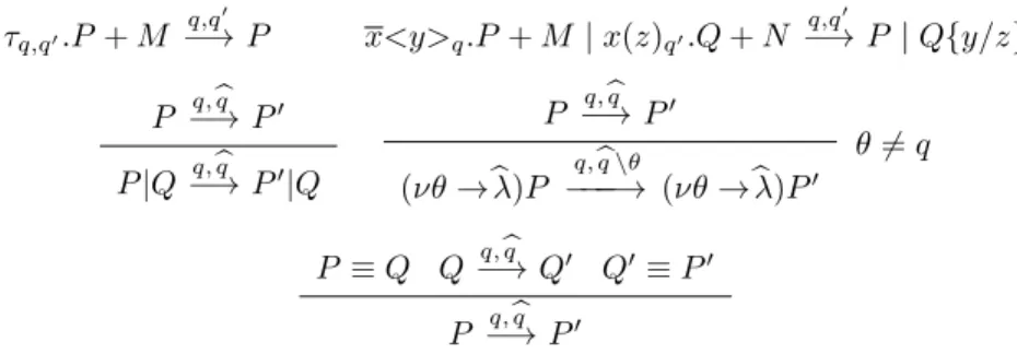
τq,q0.P + M q,q0 −→ P x<y>q.P + M | x(z)q0.Q + N q,q0 −→ P | Q{y/z} P −→ Pq,bq 0 P |Q−→ Pq,bq 0|Q P −→ Pq,bq 0 (νθ →bλ)P q, b q \θ −−−−→ (νθ →bλ)P0 θ 6= q P ≡ Q Q−→ Qq,bq 0 Q0≡ P0 P −→ Pq,bq 0
Table 8: Standard Reduction Rules with Symbolic Quantification Added
(StoOut1) P −→ σ ε /∈ {bq | P q,bq −→ } 6= ∅ (νq → λ)P −→ (νq → λ)σ ∪ {| (λ, [(νq → λ)Pq0]≡) | P q,q0 −→ Pq0|} (StoOut2) 6 ∃ σ : P −→ σ ε /∈ {q | Pb q, b q −→ } 6= ∅ (νq → λ)P −→ {| (λ, [(νq → λ)Pq0]≡) | P q,q0 −→ Pq0|} (StoIn) P −→ σ (νq)P −→ (νq)σ (StoCong) P ≡ Q Q −→ σ P −→ σ
Table 9: Stochastic Reduction Rules for Markovian Actions
4.3.2. Weighted Inputs
We consider an extension of the syntax of P, Q, . . . ∈ Pwra terms (Defini-tion 4.1) similar to the one we did, in Defini(Defini-tion 4.3, for P, Q, . . . ∈ Pra terms. The only difference is that now stochastic binders for inputs include quantification with a weight w, i.e. they are denoted by (νq → w).
Definition 4.4. We take Pwra
ext to be the set of terms P, Q, . . . generated by
extending the syntax of Pwra terms in Definition 4.1 as follows:
P ::= . . . | (νq → λ)P | (νq → w)P α ::= . . . | x<y>q | x(y)q | τq,q0
Concerning structural congruence, we consider, in addition to standard ones in Table 3, the same three laws we had for Pextra terms with the only difference
that now input prefixes and stochastic input binders are endowed with a weight w. The additional laws are thus as follows.
x<y>λ.P + M ≡ (νq → λ)( x<y>q.P + M ) if q /∈ fn(M, P )
x(y)w.P + M ≡ (νq → w)( x(y)q.P + M ) if q /∈ fn(M, P )
τλ.P + M ≡ (νq0 → w)(νq → λ)( τq,q0.P + M ) if q, q0∈ fn(M, P )/
Notice that in the last law, where, from a τ prefix, we generate stochastic names and the respective stochastic binders for a pair of (fictitious) output and input,
the choice of the weight w is not significant, in that q0 is the only input that can synchronize with the q output.
The idea behind the semantics is an elaboration of that we presented for the case of Markovian actions with non-quantified inputs. As before, in order for P −→ σ to be generated, term P must be rearranged by structural congruence in such a way that all its stochastic binders (those actually binding a prefix) are the outermost operators, with binders of inputs being outside binders of outputs they can synchronize with: under this condition, stochastic reductions P −→ σ are generated from the output binders. However now, since the input binders carry the weight information, rates included in the generated σ are represented symbolically by expressions over input stochastic names (standing for their weight): we call such a σ a symbolic rate distribution. The generated σ will be, then, turned into a usual rate distribution (i.e. a numerical one, of the kind we considered before) by traversing all the input binders (νq → w): each of them replaces the name q with the weight w inside expressions and (partially) evaluates them.
We, thus, start by introducing symbolic rate distributions to be multisets of pairs where the first element, instead of being just a rate λ ∈ RI + (as in rate distributions of Definition 3.2), is an expression E defined as follows.
Definition 4.5. We take E to be the set of expressions E generated by
E ::=P
i∈IVi| E · E | E/E
V ::= q | γ
when writing expressions we assumeP
i∈IVi with I = {k} to be simply denoted
by Vk.
We now define symbolic rate distributions. Since a rate distribution (Defini-tion 3.2) is a particular case of a symbolic rate distribu(Defini-tion (when all expressions E it includes are such that E = γ for some γ) we just extend the use of the metavariable σ to also range over symbolic rate distributions.
Definition 4.6. A symbolic rate distribution σ over a countable set S is a non-empty finite multiset over E × S, i.e. a multiset of pairs (E, e), with E ∈ E and
e ∈ S. We use SRDist(S) to denote the set of symbolic rate distributions over S.
Reduction semantics is defined, as in the case of Markovian actions with non-quantified inputs, in terms of two kind of transitions: symbolically quantified reductions P −→ Pq,bq 0, with
b
q ∈ QN ∪ {ε}, that are unchanged, i.e. still defined
as in Table 8; and stochastic reductions P −→ σ, with σ ∈ SRDist(Pwra
ext / ≡),
defined in the new Table 10.5 With respect to Table 9 considered before for
5We assume, similarly to Table 9 that (νq → λ)σ = {| (E, [(νq → λ)P ]≡) | (E, [P ]≡) ∈ σ |} and (νq → w)σ = {| (E, [(νq → w)P ]≡) | (E, [P ]≡) ∈ σ |}.
(StoOut1) P −→ σ ε /∈ Q = {q | Pb q, bq −→ } 6= ∅ (νq → λ)P −→ (νq → λ)σ ∪{|((λ·q0)/PQ,[(νq → λ)Pq0]≡) | P q,q0 −→ Pq0|} (StoOut2) 6 ∃ σ : P −→ σ ε /∈ Q = {q | Pb q, b q −→ } 6= ∅ (νq → λ)P −→ {| ((λ · q0)/P Q, [(νq → λ)Pq0]≡) | P q,q0 −→ Pq0|} (StoIn) P −→ σ (νq → w)P −→ (νq → w)(σ[w/q]) (StoCong) P ≡ Q Q −→ σ P −→ σ
Table 10: Stochastic Reduction Rules for Markovian Actions with Weighted Inputs
the version with non-quantified inputs, here we replace the rate λ in the rate distribution produced by (StoOut1) and (StoOut2) rules with the expression (λ · q0)/P Q: the rate λ of the output multiplied by the weight of the specific synchronizing input (represented symbolically by its name q0) and divided by the sum of the weights of all the inputs it can synchronize with (represented
symbolically by P Q). Concerning the latter, we assume P Q to stand for
P
i∈Iqi (belonging to the syntax of expressions E) by considering any name
indexing qisuch that Q = {q1, . . . , qn}. Moreover the rule (StoIn) is now changed
by considering, in its target, σ[w/q] instead of the same distribution σ considered in its premise. In Table 10 we assume σ[w/q] to be defined as the symbolic rate distribution obtained by replacing every expression E occurring inside σ with E[w/q], i.e. σ[w/q] = {| (E[w/q], e) | (E, e) ∈ σ |}. In turn we assume E[w/q] to be the expression obtained from E by first replacing occurrences of name q in E with value w and by subsequently computing all its operations that include no names in their arguments. Formally, we define E[γ/q] as eval (E{γ/q}) where: E{γ/q} is the expression E0 obtained by syntactically replacing all occurrences of q ∈ QN with γ ∈ RI +inside E, and the eval function is defined as follows.
Definition 4.7. Function eval from E to E , that (partially) evaluates an expres-sion E yielding an expresexpres-sion E0, is defined by
• eval (γ) = γ • eval (q) = q
• eval (γ0· γ00) = γ where γ is the result of γ0· γ00
eval (E1· E2) = eval (E1) · eval (E2) if 6 ∃γ0, γ00: E1= γ0∧ E2= γ00
• eval (γ0/γ00) = γ where γ is the result of γ0/γ00
eval (E1/E2) = eval (E1)/eval (E2) if 6 ∃γ0, γ00: E1= γ0∧ E2= γ00
• eval (P
i∈Iγi) = γ where γ is the result ofPi∈Iγi
eval (P
i∈IVi) =Pi∈IVi if 6 ∃{γi| i ∈ I} : ∀i ∈ I. Vi= γi.
Notice that, since in transition systems we consider stochastic reductions P −→ σ only for terms P ∈ Pextwra such that there exists P0 ∈ Pwra with
P ≡ P0, we have that P −→ σ implies that σ is a (numerical) rate distribution (Definition 3.2). This is a consequence of the fact that, in such terms P , partial evaluations made by input stochastic binders lead us to completely evaluate the expressions inside the generated symbolic rate distribution once the top-level of term P is reached. This will be proved formally in the following (Proposition 4.2). Example 4.4. Consider again term P = x<y>3.P0|(x(z)4.P00|x(z0)8.P000) of
Example 4.2. Let us now apply our reduction semantics to P . We have that P ≡ (νq0→ 4)(νq00→ 8)(νq → 3)(x<y>q.P0|(x(z)q0.P00|x(z0)q00.P00))
thus P performs the stochastic transition
P −→ {|(1, [P1]≡), (2, [P2]≡)|}
where P1 and P2 are those of Example 4.2.
4.3.3. Basic Properties
We now discuss basic properties of reduction semantics for π-calculus with Markovian actions presented in previous Sections 4.3.1 and 4.3.2, i.e. encom-passing both considered versions: with and without weights. As we did in Section 4.2.3, we use P[w]ra inside definitions/propositions to mean that the
definition/proposition holds both when we take it to be Pra and, also, when we
instead consider Pwra.
We first observe that, as for the case of Markovian delays, the transition system of terms given by the reduction semantics can be represented in a finitary way by taking states to be congruence classes [P ]≡∈ P
[w]ra
ext / ≡. This is obtained
by using the following definition (also here it would have been possible to modify reduction semantics rules so to make them work directly on congruence classes, as explained in Section 3.2).
Definition 4.8. Let P, P0∈ Pext[w]ra. We define [P ]≡ q, bq −→ [P0]≡whenever P q, bq −→ P0. Let P ∈ Pext[w]ra and σ ∈ SRDist(Pext[w]ra/ ≡). We define [P ]≡ −→ σ whenever
P −→ σ.
Notice that, in the case of P ∈ Pra
ext, we also have that σ ∈ RDist(Pextra/ ≡).
We now analyze properties of (outgoing) transitions of terms P[w]ra ∈ P, that is, terms belonging to the non-extended syntax, similarly to what we did for the case of Markovian delays in Section 3.3. Also here, since congruent terms have the same outgoing transitions, the presented properties obviously hold also for terms P ∈ Pext[w]rasuch that P ≡ P0 for some P0∈ P[w]ra.
The following proposition is analogous to Proposition 3.1, the difference being that it considers −→ transitions instead ofq,bq −→ transitions.q
Proposition 4.1. Let P ∈ P[w]ra. There is no P0 ∈ P[w]ra
ext , q ∈ QN ,q ∈b QN ∪ {ε} such that P −→ Pq,bq 0.
Proof. A direct consequence of the fact that for any Q ≡ P , with P ∈ P[w]ra, we have that, due to the laws of ≡, all prefixes “x<y>q” and “τq,q0” occurring in
Q are bound by a (νq → λ)P binder (rules for (νq → λ)P binders do not allow
transitions −→ labeled with the bound name q to be inferred).q,bq 2
The following proposition is analogous to Proposition 3.2. Here we addition-ally state that P −→ σ, with P belonging to the non-extended syntax, implies that σ is a (numerical) rate distribution (Definition 3.2). This is significant only for the version with weights and means that, for terms P ∈ Pwra, symbolic rate
distributions (that are not rate distributions) are used only during inference of stochastic reductions.
Proposition 4.2. Let P ∈ P[w]raand P −→ σ. We have σ ∈ RDist(Pext[w]ra/ ≡) and P −→ σ0 implies σ = σ0.
Proof. The proof, reported in Appendix B, is an elaboration of that of Proposi-tion 3.2. It is, however, much more involved also due to the interplay between stochastic output binders and stochastic input binders, which, in the variant with input weights, additionally entails rate calculation by means of symbolic
rate distributions during stochastic transition inference. 2
The following proposition is analogous to Proposition 3.3, the difference being that it considers terms P0 that are reachable just by P −→ σ transitions (we no longer have P −→ P0 transitions).
Proposition 4.3. Let P ∈ P[w]ra and P0 ∈ Pext[w]ra such that P −→ σ ∧ ∃λ : (λ, [P0]≡) ∈ σ. There exists P00∈ P[w]ra such that P00≡ P0.
Proof. For any Q ≡ P with P ∈ P[w]ra we have: all named prefixes “x<y>q”,
“x(y)q” and “τq,q0” occurring in Q are bound and every stochastic binder can
bind at most a single named prefix. It is easy to verify that this property is preserved by transitions Q −→ σ for which ∃λ such that (λ, [Q0]
≡) ∈ σ, i.e. for
any such Q0 the same property holds true. Performing the σ transition causes, for instance, the corresponding pair of stochastic binders not to bind any named prefix in the target state.
Any Q0 satisfying the property above can be shown to be congruent to a term of P by just removing stochastic binders not binding any delay prefix and by turning bound named prefixes into Markovian action prefixes: x<y>λ, τλ and
x(y) (or x(y)wfor the version with weights). 2
As in the case of Markovian delays, a consequence of the above propositions and of Definition 4.8 is that, given P ∈ P[w]ra, we can represent the semantics of P as a transition system over states [P0]≡ such that P0 ∈ P[w]ra (with the
initial state being [P ]≡).
Concerning the underlying Markov Chain we consider the rate γ([P ]≡, [P0]≡)
in Section 3.2, that is: P (λ,[P0] ≡)∈σλ · µσ(λ, [P 0] ≡) if [P ]≡ −→ σ for some σ; 0 otherwise.
The above also provides a definition of bisimulation over states of P ∈ P[w]ra by applying it to Definition 4.2 and by assuming: γ([P0]
≡, τ, [P00]≡) =
γ([P0]
≡, [P00]≡), for any P0, P00 ∈ Pext[w]ra and γ([P0]≡, µ, [P00]≡) = 0, for any
µ 6= τ and P0, P00∈ Pext[w]ra. Again, obviously, w.r.t. the Markov Chain obtained by labeled operational semantics, reduction semantics of a term P yields a closed system interpretation, i.e. as if all (free) actions of P were bound at the top level. 4.4. Comparison Results
We now compare, for each of the two versions of the π-calculus presented in Section 4.1, our reduction semantics with classical labeled semantics, similarly to what we did for Markovian delays.
The version without weights satisfies a Harmony theorem similar to Theo-rem 3.1.
Theorem 4.1 (Harmony). Let P ∈ Pra. We have P −→ σ for some σ iff
P −−−τλ−→ P,id 0 for some λ, id and P0. Moreover, when both hold, we have that
∀P0∈ Pra X (λ,[P0]≡)∈σ λ · µσ(λ, [P0]≡) = X P τλ,id−−−→−−−−−−− ≡P0 λ
Proof. The proof, reported in Appendix B, is based on that of Proposition 4.2 in a similar way to how the proof of Theorem 3.1 relates to that of Proposition 3.2: it exploits the detected structure of the unique σ (if any) such that P −→ σ. However here we need to resort to more complex machinery, also due to the interplay between stochastic output binders and stochastic input binders. 2 Theorem 4.1 also confirms what is shown in [12], i.e. that for terms P ∈ Pra with the classical approach (where the notion of apparent rate is not used) parallel is associative up to Markovian bisimulation: if in Example 4.1 we associate parallel to the left we still get two τ2transitions (only id labels change).
For the version with weights, instead, Theorem 4.1 does not hold: as we discussed in the Introduction this is related to the fact that, differently from our approach (where we always consider the total weight of all input actions synchronizable with a given output), parallel of Stochastic π-calculus [21] is not associative [12]. If we consider Q = (x<y>3.P0|x(z)4.P00)|x(z0)8.P000, i.e. P
of Example 4.2 where parallel is, instead, associated to the left, the classical approach yields (differently from P that performs a τ1 and a τ2transition) two
τ3 transitions distinguished just by the id label. This provides a counterexample
that shows that Theorem 4.1 does not hold for terms P ∈ Pwra(Q obviously has the same stochastic transition as P , we showed in Example 4.4, in that P ≡ Q).