HAL Id: hal-00459261
https://hal.archives-ouvertes.fr/hal-00459261
Submitted on 23 Feb 2010
HAL is a multi-disciplinary open access archive for the deposit and dissemination of sci-entific research documents, whether they are pub-lished or not. The documents may come from teaching and research institutions in France or
L’archive ouverte pluridisciplinaire HAL, est destinée au dépôt et à la diffusion de documents scientifiques de niveau recherche, publiés ou non, émanant des établissements d’enseignement et de recherche français ou étrangers, des laboratoires
Modeling the latency on production grids with respect
to the execution context
Diane Lingrand, Tristan Glatard, Johan Montagnat
To cite this version:
Diane Lingrand, Tristan Glatard, Johan Montagnat. Modeling the latency on production grids
with respect to the execution context. Parallel Computing, Elsevier, 2009, 35 (10-11), pp.493–511. �10.1016/j.parco.2009.07.003�. �hal-00459261�
Modeling the latency on production grids
with respect to the execution context.
Diane Lingrand
a,∗, Tristan Glatard
b, Johan Montagnat
aaI3S University of Nice - Sophia Antipolis / CNRS - FRANCE
bUniversity of Amsterdam Institute of Informatics/Academic Medical Center
-THE NE-THERLANDS
Abstract
In this paper, we study grid jobs latency. Together with outliers, latency highly im-pacts applications performance on production grids, due to its order of magnitude and important variations. It is particularly prejudicial for determining the expected duration of applications handling a high number of jobs and it makes outliers de-tection difficult.
In a previous work, a probabilistic model of the latency has been used to estimate an optimal timeout value considering a given distribution of jobs latencies. This timeout value is then used in a job resubmission strategy.
The purpose of this paper is to evaluate to what extent updating this model with relevant contextual parameters can help to refine the latency estimation. In the first part of the paper, we study the validity of parameters along several weeks. Experiments on the EGEE production grid show that performance can be improved by updating model parameters. In the second part, we study the influence of the resource broker or the computing site and the day of the week. We experimen-tally show that some of them have a statistically significant influence on the job latency. We exploit this contextual information in the perspective of improving job submission strategies.
Key words: grid computing, production grid, execution context
∗ Corresponding author.
Email address: [email protected] (Diane Lingrand). URL: www.i3s.unice.fr/~lingrand (Diane Lingrand).
1 Motivations
Users often complain on low efficiency and faults encountered on production grids. For instance, running metagenomics experiments on EGEE, authors of
[ABEHG08] report 8% of non finished jobs (pending forever), 27% of aborted
jobs (mainly due to credentials expiration) and 65% of finished jobs. On those finished jobs, only 45% were correctly completed, due to different problems: file transfer errors, file catalog error, uploads and installation problems. Production grids are characterized by high and non-stationary load and by a large geographical expansion. As a consequence, latency, measured as the duration between the beginning of a job submission and the time it starts executing, can be very high and prone to large variations. As an example,
on the EGEE (Enabling Grid for E-sciencE) production grid1, the average
latency is in the order of 5 minutes with standard deviation also in the order of 5 minutes. This variability is known to highly impact application performance
and thus it has to be taken into account [SB99].
Modeling grids latency is interesting to give a reliable estimation of the ex-pected jobs completion time. On an unreliable grid infrastructure where a significant fraction of jobs is lost (outliers), this information is valuable to set up an efficient resubmission strategy minimizing the impact of faults. It can be exploited either at the workload management system level or at the user level. Jobs facing too high latencies are cancelled and resubmitted before they become too penalizing.
In [GMP07], a probabilistic model is presented to allow the optimization of
timeout values considering a given latency distribution. This timeout value is then used for job resubmission. In this paper, we test the validity of such a model along time.
In previous works [GLMR07, LMG08], we have shown that some parameters
of the execution context have an influence on the cumulative density function of the latency. In this paper, we quantify their influence on the timeout values and the expected execution time (including resubmissions). We aim at refining our model by taking into account most relevant contextual parameters in order to optimize job resubmission strategies.
Section 2 presents several initiatives aiming at modeling grid infrastructures
and, in particular, several studies on the influence of different parameters. In this work, we focus on a particular production grid, EGEE, that is described
in section3. Section4introduces our latency model including job resubmission
in case of faults or outliers. This model aims at determining the best value of 1 EGEE,http://www.eu-egee.org/
job timeout and is based on real observations on a production grid. The data that has been used for the experiments proposed in the paper is described in
section 5. The experiments are presented in the next two sections. Section 6
studies the validity of our model along time and shows that an update of the estimated model parameter is valuable for reducing the global latency.
Section7studies the influence of different parameters of the execution context
on the estimated model parameters and the global latency. Resource brokers, computing centers, day of the week and time of the day are considered.
2 Related work
Several initiatives aim at modeling grid infrastructure Workload Manage-ment Systems (WMS). They are usually based on logs from local clusters
[CGV08,GLMT08] or national grids [LGW04,NPF08] or probe jobs for
mea-surements [GLMR07]. Some initiatives aim at collecting large collection of
logs. The Network Weather Service [SW04] proposes an architecture for
man-aging large amounts of data in the purpose of prediction making. The Grid
Workloads Archive [ILJ+08] proposes a workload data exchange format and
associated analysis tools in order to share real workload from different grid environments. It already contains more than 7 billions data entries. More
re-cently, the Real Time Monitor (RTM)2 together with the Grid Observatory3
propose extensive traces from the EGEE grid. These traces were not avail-able at the time of the experiments made in this paper. They also require pre-processing such as data cleaning and interpretation in order to be used.
This explains why we have used probe jobs (detailed in section 5) for the
experiments of this paper. In addition, probe jobs submitted from the user environment, exactly relate to what is experienced from her point of view. Taking into account contextual information has been reported to help in es-timating single jobs and workflows execution time by rescheduling. Different works have been done on either experimental or production grid. Feitelson
[Fei02] has pointed out the importance of these studies and the methodologies
to conduct them.
We now detail several works that have studied the influence of different param-eters, detected or measured on experimental or production grids, with different types of resources (dedicated, shared, ...) and with very different load patterns. Some works have used these parameters to better model the studied factors while others have only observed their influence, without extracting models. 2 Real Time Monitor, http://gridportal.hep.ph.ic.ac.uk/rtm
Feitelson [Fei02] observed correlations between run time and job size,
num-ber of clusters and time of the day. In [NDG06], the influence of changes in
transmission speed, in both executable code and data size, and in failure like-lihood are analyzed for a better estimation of end time of sub-workflows. This information is used for re-scheduling jobs after faults or overruns.
In [LGW04], correlations between job execution properties (job size or number
of processors requested, job run time and memory used) are studied on a multi-cluster supercomputer in order to build models of workloads, enabling
comparative studies on system design and scheduling strategies. In [NMB+06],
authors make predictions of batch queues waiting time to improve the total execution time.
To refine grid monitoring, [RBJS06] presents a model of the influence between
the grid components and their execution context (system and network levels), experimented on the Grid’5000 French national platform.
In [NPF08], authors constructed a model for the prediction of resource
avail-ability on the Austrian grid. Their study of the impact of the day of the week and the hour of the day clearly shows two different profiles. The differences with our work are that users of this grid are all located in Austria (same timezone, similar working periods) and that this grid does not seem to be saturated, contrarily to the EGEE one.
Authors of [OCV07] analyze job inter-arrival times, waiting times in the
queues, execution times and size of exchanged data. They conducted experi-ments on the EGEE production grid on several VOs (Virtual Organizations) and studied the influence of the day of the week and the time of the day. Their conclusion is that the load increases at the end of the day but that it is difficult to extract a precise model of this behavior with respect to the day or to the time.
Users behavior on the EGEE grid is studied in [DCDO07]. The authors
ob-served that “some job submissions are done during the morning, and most of them are done in the afternoon”, with a ratio of more than two. However, authors are not proposing strategies to exploit this information.
These works present studies on different factors such as inter-arrival time, batch queues waiting time, latency, execution time or availability of resources. They all depend on the load of the grid. The parameters that have been studied can be divided in different categories:
Job context: run time, memory used, number of processors requested and data size required.
Execution environment context: system, network (architecture, proto-col, bandwidth, transmission speed), day of the week and hour of the day.
In the remainder of this paper, we focus on heavily loaded production grids for implementing a resubmission strategy. Our work focus on the estimation of the latency impacting jobs prior to their start time which is notified by the middle-ware. The resubmission strategy does not require taking into account the jobs context but only their execution environment context. Resource brokers and computing centers batch systems are the first parameters that we will study.
In addition, taking into account observations of [DCDO07, NPF08] together
with our own observations, day and time of submission will be studied. We will now describe the EGEE production grid used has experimental plat-form in order to introduce the different elements involved in the latency and job submission.
3 Experimental platform
Our experiments are conducted within the biomed VO of the EGEE produc-tion grid infrastructure. With 40,000 CPUs dispatched world-wide in more than 240 computing centers (at the time of the experiments), EGEE represents an interesting case study as it exhibits highly variable and quickly evolving load patterns that depend on the concurrent activity of thousands of potential users. Even if the infrastructure is relatively homogeneous from the OS point of view (all the hosts are running Scientific Linux, based on Red-Hat distribu-tion), important architecture and performance variations are expected among the worker nodes (64/32 bits machines, single/multiple processors, different speeds, single/multiple cores).
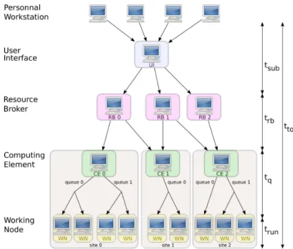
On the EGEE grid, when a user wants to submit a job from her workstation,
she connects to an EGEE client known as a User Interface (see figure 1). A
Resource Broker (RB) queues the user requests and dispatches them to the available computing centers. The gateway to each computing center is one or more Computing Element (CE). A CE hosts a batch manager that distributes the workload over the Worker Nodes of the center. Different queues handle jobs with different forecast wall clock times. The policies for deciding on the number of queues and on the maximal time assigned to each of them are site-specific. We later denote as CE-queue a specific batch queue configured on a given CE.
During its life-cycle, a job is characterized by its evolution status. If everything happens as expected, the job is then completed. Otherwise, it might be aborted,
timed-outed or in an error status depending on the type of failure.
The latency is measured as the duration between the beginning of a job
Fig. 1. EGEE job life cycle: from the submission by a user on her personal work-station to the working node where the job will run.
to the middleware architecture, an incompressible polling delay is necessary
to detect the job termination after trun. When detecting the running state of
a job, the measure is subject to this polling time which is therefore integrated into our measurements. In the remainder, we will call latency the total delay experienced by the user, including the polling time.
In a typical application of the biomed VO, the mean and standard-deviation of the latency have similar values, in the order of magnitude of job execution times (several minutes, up to hours). Thus, the latency and its variations have an important impact on the performance. A precise model of the latency is needed to handle failed jobs and refine submission strategies.
4 Using latency models for optimization
Models of the grid latency enable the optimization of job submission
parame-ters such as job granularity [GMP06] or timeout value, which can improve the
robustness of the WMS against system faults and outliers.
Properly modeling a large scale infrastructure is a challenging problem given
its heterogeneity and its dynamic behavior. In a previous work [GMP08], we
adopted a probabilistic approach which proved to be able to explain applica-tion performance on a producapplica-tion grid.
In [GMP07], we have shown how the distribution of the grid latency impacts
the choice of a timeout value for the jobs. We model the grid latency as a
random variable R with probability density function (pdf) fR and cumulative
density function (cdf) FR. Outliers are jobs that did not returned. We denote
by ρ the ratio of jobs considered as outliers. The strategy we consider consists in cancelling and resubmitting a job when it has not reached the running status
before a certain time, called timeout and denoted by t∞. As demonstrated in
detail in appendix A, the expectation of the resulting of the total latency J
faced by the job (including resubmissions) is expressed as a function of R, the
timeout t∞ and the proportion of outliers ρ:
EJ(t∞) = 1 FR(t∞) t∞ Z 0 ufR(u)du + t∞ (1 − ρ)FR(t∞) − t∞ (1)
EJ is denoted as the “expected execution time” in the remainder of the paper
since we consider jobs of almost null execution time. The optimal timeout
value is obtained by minimizing EJ with respect to the timeout value t∞.
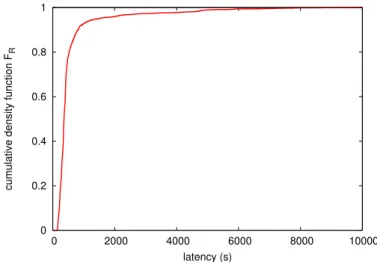
0 0.2 0.4 0.6 0.8 1 0 2000 4000 6000 8000 10000
cumulative density function F
R
latency (s)
Fig. 2. Cumulative density function (FR) of the latency for all jobs completed before
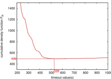
400 496 600 800 1000 1200 1400 200 300 400 500 528 600 700 800 900 1000
cumulative density function F
R
timeout value(s)
Fig. 3. Expected execution time with respect to the timeout value. In this example, the minimum of the curve is reached for t∞= 528s, leading to the shortest execution
time EJ = 494s.
a set of 5,800 measurements. Figure 3 plots EJ with respect to the timeout
value t∞, using equation1. The curve presents a fast decreasing phase towards
a minimal followed by a slow increasing phase. The increasing phase tends towards an asymptotic straight line which slope increases with the fraction of outliers (here, 3%). The minimum of the curve gives the optimal timeout value
(here, t∞= 528s leading to EJ = 494s). Underestimation of the timeout value
leads to a higher increase of the expected execution time than overestimation.
Given a probability distribution of the latency, minimizing equation 1 gives
the best choice for the timeout value. In the real life, we will have to first measure the probability distribution in order to compute the optimal timeout
value. In a first step (Section 6), we will study the validity of the model
along time and the frequency of necessary updates. Then, we will focus on refining this model by considering parameters of the execution context that can be identified during the job life cycle: the target Resource Broker (RB), the Computing Element (CE) and finally the local submission date and time
(Section7). The goal is to exhibit parameters for which we obtain significantly
different optimal timeout values. Those parameters could then be included into optimization strategies to improve their accuracy, thus leading to better performance.
5 Experimental data and method
To study grid latency, measures were collected by submitting a significant number of probe jobs. These jobs, consisting in the execution of a negligible duration /bin/hostname command, are only impacted by the grid latency. In
the remainder we make the hypothesis that the users job execution time is known and that therefore only the grid latency varies significantly between different runs of the same computation task. To avoid influencing the system load with our monitoring, a constant number of probes was maintained inside the system at any time during the data collection: a new probe was submitted each time another one completed. For each probe job, we logged the job sub-mission date, the job final status and the total duration. The probe jobs were assigned a fixed 10,000 seconds maximal duration beyond which they were considered as outliers and cancelled. This value is far greater than the average latency observed (in the order of 300 seconds). We consider as faults both outliers jobs and jobs that really failed before 10,000 seconds. We compute
the ratio of faults and introduce it as the ρ value in equation 1, considering
that all faults are resubmitted at t∞.
In a previous work [GLMR07], we collected 5,800 job traces in September 2006
(denoted further as 2006-IX). In this paper, we added 10,000 job traces (with an outliers ratio of 21%) acquired between September 2007 and March 2008. The exact periods of experiment are thus:
• September 15th 2006 until September 26th 2006 (2006-IX)
• September 5th 2007 until September 27th 2007 (weeks 2007-36 to 2007-39) • December 12th 2007 until December 17th 2007 (week 2007-50)
• December 21th 2007 until January 22th 2008 (weeks 2007-51 to 2008-03) • February 15th 2008 until March 11th 2008 (weeks 2008-07 to 2008-10) The discontinuity of the periods in the later data set is due to unscheduled failures in the acquisition system and does not have any relation with authors choices.
In the study we are conducting, we aim at reducing the total execution time including resubmissions when failures happen. For studying the influence of a parameter, we split the data according to the studied parameter into different subsets indexed by i. The studied parameters and the corresponding meaning for i are:
validity for long period of time: number of the week (see section 6)
resource broker: index of the RB in the list of RBs (see subsection 7.1)
computing element and queue: index of the class of CE-queue (see
sub-section7.2)
day of the week: number of the day in the week (1-7) (see subsection 7.3)
hour of the day: index of the 4 hours time period in the day (1-6) (see
subsection7.4)
working versus non working periods: boolean value
The model (random variable Fi, optimal t∞i conducting to the minimal EJ i) is
is thus compared to the value obtained with the optimal timeout computed
from the whole data set: EJ i(t∞all). The relative difference:
∆ = EJ i(t∞i) − EJ i(t∞all) EJ i(t∞all)
expresses the reduction of the execution time yielded by adapting the opti-mization strategy to the studied parameter.
We first study the validity of the model parameters for long periods of time by splitting the data into subsets corresponding to single weeks. In this study, we
have computed a ∆EJ instead of the above ∆, considering that, in practice,
parameters will be estimated at a certain time and used during a later period
of time. The expression of ∆EJ is given by:
∆EJ = EJ i(t∞i) − EJ i(t∞j) EJ i(t∞j)
where j corresponds to the reference subset.
6 Study of the validity of model parameters along time
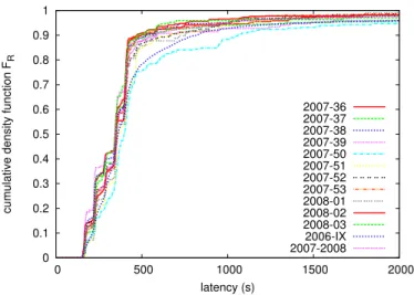
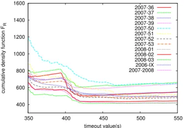
Figure4shows the cumulative density function of the latency for the different
weeks and for the whole period of 2007-2008. The curves covering the period 2007-2008 present a similar profile. We observe that most of the times, the distribution of the job waiting times in the RB is multi-modal, thus
explain-ing the steps on figure4. These modes could be due to the internal scheduling
algorithm of resource brokers. Another possible cause might be the RB imple-mentation itself (e.g. presence of active polling loops, etc.). Such steps have
also been observed by other biomed users (see e.g. figure 4 in [ABEHG08])
and in the vlemed VO of the EGEE grid.
An interesting way to compare those curves is to consider the differences be-tween the optimal timeout values that they led to (computed using
equa-tion 1). Figure 5shows the expectation of the execution time for the different
weeks. Despite the fact that the curves have different profiles, the optimal timeout values are visually in the same interval, around 400s.
These values are detailed in table 1: the optimal value for 2006 is 528s while
values for 2007-2008 range between 422s and 491s. The table also displays, for each period of time, the mean value and the standard deviation of the latency R. In most cases, a reduction of the mean latency corresponds to a decrease of
0 0.1 0.2 0.3 0.4 0.5 0.6 0.7 0.8 0.9 1 0 500 1000 1500 2000
cumulative density function F
R latency (s) 2007-36 2007-37 2007-38 2007-39 2007-50 2007-51 2007-52 2007-53 2008-01 2008-02 2008-03 2006-IX 2007-2008
Fig. 4. Cumulative density function of the latency for each week, computed on completed jobs. 0 500 1000 1500 2000 2500 3000 0 500 1000 1500 2000
cumulative density function F
R timeout value(s) 2007-36 2007-37 2007-38 2007-39 2007-50 2007-51 2007-52 2007-53 2008-01 2008-02 2008-03 2006-IX 2007-2008
Fig. 5. Expectation of job execution time with respect to the timeout value (t∞).
The minimum of each curve gives the best timeout value for the considered data set.
400 600 800 1000 1200 1400 1600 350 400 450 500 550
cumulative density function F
R timeout value(s) 2007-36 2007-37 2007-38 2007-39 2007-50 2007-51 2007-52 2007-53 2008-01 2008-02 2008-03 2006-IX 2007-2008
date R¯ σ(R) outliers best t∞ EJ(t∞) 2006-IX 570s 886s 5% 528s 494s 2007/08 469s 723s 17% 474s 500s 2007-36 446s 748s 24% 423s 502s 2007-37 506s 848s 33% 422s 606s 2007-38 447s 682s 24% 428s 522s 2007-39 489s 741s 32% 436s 585s 2007-50 660s 1046s 18% 467s 628s 2007-51 478s 510s 13% 491s 510s 2007-52 443s 582s 13% 482s 469s 2007-53 449s 678s 16% 484s 482s 2008-01 434s 317s 13% 485s 491s 2008-02 418s 547s 12% 433s 435s 2008-03 538s 1196s 10% 474s 413s Table 1
Mean and standard variation of the latency, fraction of outliers, optimal timeout value and minimal expectation of execution time. These quantities are computed for the 2006 period, for the 2007-2008 period and for all weeks in the 2007-2008 period. The minimal optimal timeout value is 422s while the maximal one is 491s.
the standard deviation. Finally the optimal expected execution time is shown. Assuming that the optimal timeout value has been computed in September
2006 (528s), we compute, in table 2, the resulting expectation of execution
time and the relative difference with the optimal value computed week by week in order to measure the impact of parameters chosen earlier instead of the optimal ones. The relative differences are up to 8%. It happens that this timeout value is higher than all optimal values for the period 2007-2008. The
highest differences are obtained when the ascending slopes of figure 5are the
highest, which is directly related to the fraction of outliers.
Furthermore, if we consider the minimal and the maximal of timeout values among the different weeks (422s and 491s), the expected execution time for
each of these values and the relative differences are shown in table 3. In the
case of the maximal timeout value, relative errors are below 6% while in the case of the minimal timeout value, relative errors are up to 17%. This is clearly
explained by the shape of the curves on figure 5: the slope of the decreasing
part is higher than the slope of the increasing part of each curve. Thus, an overestimation of the timeout value is better than an underestimation, if this overestimation is not too high, which must be quantified. As a conclusion of
date EJ(528s) ∆EJ date EJ(528s) ∆EJ 2007-36 528s 5.2 % 2007-52 477s 1.7 % 2007-37 648s 7.0 % 2007-53 491s 1.9 % 2007-38 544s 4.2 % 2008-01 493s 0.4 % 2007-39 631s 7.9 % 2008-02 441s 1.4 % 2007-50 652s 3.9 % 2008-03 418s 1.2 % 2007-51 514s 0.9 % Table 2
In this experiment, the timeout value from the period of September 2006 has been used (528s). For each week of the 2007-2008 period, we present the expectation of the execution time and the relative difference with the optimal one.
date EJ(422s) ∆EJ% EJ(491s) ∆EJ% 2007-36 505.5 0.7% 527.1 5.0% 2007-37 605.9 0% 632.2 4.3% 2007-38 524.8 0.5% 530.5 1.6% 2007-39 602.9 3.1% 616.8 5.5% 2007-50 718.7 14.5% 642.3 2.3% 2007-51 594.9 16.7% 509.6 0% 2007-52 491.2 4.8% 470.9 0.4% 2007-53 513.4 6.5% 484.0 0.4% 2008-01 516.7 5.2% 493.1 0.4% 2008-02 437.0 0.6% 437.2 0.6% 2008-03 419.1 1.5% 414.8 0.5% Table 3
In this experiment, we focus on data from the period 2007-2008. As determined in table 1, the minimum timeout value is 422s and the maximum is 491s. For these extreme values, the new expectation of execution time and the relative difference with the optimal value are presented.
this part of the study, updating the timeout value along time may improve the total execution time, up to 17%.
7 Latency context parameters
In order to refine our model, we consider the parameters of the execution con-text that could explain the high variability of the latency. Two different jobs submitted on the EGEE grid may differ on the path they follow from their sub-mission site (UI) to the execution site (WN). Different hardware characteristics and software configurations/versions may also influence the performance. The load of the infrastructure is also an important factor and may depend on the behavior of the users and on the nature of the experiments they are conduct-ing. Not only users are to be considered but also administration operations that influence the grid status. Similarly, time context (working or non-working periods) is to be considered. Failures may have different explanations such as hardware failures, load and any other external factors (such as extremely hot weather conditions leading to air conditioning failures, . . . ).
Going into the details of all the local parameters of the problem is intractable due to the difficulty to acquire and store such information. The level of details that can be exploited depends both on the availability of the contextual
infor-all RBs RB fr RB es RB ru optimal t∞ t∞ref = 556 s 729 s 546 s 506 s ∆t∞ 0% 31% 2% 9% min EJ 479.125 s 483.7 s 445.2 s 476.2 s EJ(t∞ref) 479.125 s 488.8 s 445.9 s 477.9 s ∆EJ 0% 1% 0.2% 0.4% Table 4
Study of the influence of the Resource Brokers.
mation and on the needs of the model. We thus restrict our study to context parameters that could realistically be used for estimating job latencies and op-timizing job resubmission strategies. In the following, we consider high level information such as Resource Broker, Computing Element and queues used. We also study the time context using the day of the week, and time periods of the day.
7.1 Resource Broker parameter (RB)
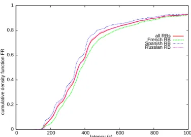
The probe measures acquired during three weeks in September 2006 (log 2006-IX) were submitted to 3 different Resource Brokers (RBs):
• a French one (grid09.lal.in2p3.fr), • a Spanish one (egeerb.ifca.org.es) and • a Russian one (lcg16.sinp.msu.ru).
In this log, the outlier ratio ρ was 5%. Figure7displays the cumulative density
function of the latency of the probe jobs sent to each of the RBs as well as the one of the submission time considering all RBs.
The 3 RBs exhibit quite different behaviors that need to be quantified. Table4
displays in each row:
• the optimal estimated timeout value;
• the difference between this value and the global reference value obtained using all measurements without distinction between RBs;
• the minimal expected execution time;
• the expected execution time if the timeout is set to the global reference value;
• and the relative difference with the optimum.
The optimal timeout values significantly differ and the most distinct is the one
0 0.2 0.4
cumulative density function FR
0.6 0.8 1 0 200 400 latency (s) 600 800 1000 all RBs French RB Spanish RB Russian RB
Fig. 7. Cumulative density function for the different Resource Brokers: France (fr), Spain (es) and Russia (ru).
0 500 1000 1500 2000 2500 3000 0 200 400 600 800 1000
expectation of execution time E
J (s) timeout value(s) all RBs French RB Spanish RB Russian RB
execution time varies by a much smaller amount (∆EJ <1%). This shows that even if a parameter (here the RB) might significantly influence the time-out optimization, its impact on the execution time is not necessarily critical. Taking into account the RB in the timeout optimization will not improve the execution time, compared to the regular update of the model parameters.
7.2 Computing Element (CE)
In a computing center, the batch submission system is usually configured with several queues. The influence of the Computing Element (CE) and the associ-ated queues (CE-queue), is considered in this section. The same methodology
as in section 7.1 could be envisaged but a significant difference is that the
number of CE-queues is much higher than the number of RBs in the same set of data: we had 92 CEs and queues and only 3 RBs. It might thus be relevant
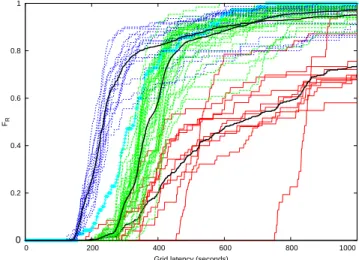
to group similar CE-queues to obtain fewer classes. As can be seen in figure9
many of the 92 CE-queues have similar cdfs while others are more singular. The idea here is to group CEs and queues that have similar properties into different classes. To ensure statistical significance, CE-queues with less than
0 0.2 0.4 0.6 0.8 1 0 200 400 600 800 1000 FR
Grid latency (seconds)
Fig. 9. Classification in 3 classes of the cumulative density functions of the grid latencies by CE. Centroids of the k-means classes are plotted in black.
30 probe measures were removed from the study. Sixty (60) CE-queues out of the 92 remained.
7.2.1 Methodology
As explained at the end of section 5, we are interested in splitting the data
in different subsets and to evaluate the pertinance of the parameters deter-mining this clustering. We have used the k-means classification method that
classification, we have used a well known method: ANOVA that we detail in
paragraph 7.2.1.2.
In subsection 7.2.2, we build three classes from intuitive observations on the
distribution profiles. We refine this analysis by studying different number of
classes from 2 to 10 in subsection 7.2.3. ANOVA analysis shows that H0 is
rejected in all cases but refining results from the case of 3 classes (subsection
7.2.4) shows that only 2 classes are statistically different. We conclude by
merging 2 classes obtained from the classification into 3 classes and comparing the result with the classification into 2 classes.
7.2.1.1 Classification method: k-means The k-means method [Ste56]
is an iterative method that clusters data in k different classes by minimizing the intra cluster variance (the sum of squared distance of the elements of a class to its centroid). This method is very fast but needs to specify the number of classes, value k, and an initialisation of each centroid.
The distance we have used is a distance between two curves FR and is
com-puted as the sum of the squared distance between FR values for same latency
values. Different values of k have been studied in this paper. For evaluation of the classification result, the ANOVA method has been used.
7.2.1.2 Evaluation of the classification: ANOVA The ANalysis Of
VAriance (ANOVA) [Fis25] is a well-known method in statistics that consists
in a generalisation of the T-test for more than two subsets of a dataset and
that tests an hypothesis usually called H0, the null hypothesis. This hypothesis
says that the subset data were drawn from the same population. The ANOVA test compares the variance of the different subsets with the variance of the whole dataset, using a ratio F , in order to validate or not the null hypothesis:
F = variance between groups
variance within groups
Depending on the F value and the degree of freedom, Df , of the problem, a
confidence in rejection of H0 is given, usually denoted by p. In the case of our
study, the degree of freedom is given by the number of classes minus 1. From such an analysis, if the rejection is confirmed, it does not say that all classes are statistically different, but only that they are not similar. Further tests must be done in order to determine how many subsets are statistically different.
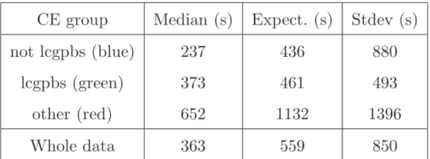
CE group Median (s) Expect. (s) Stdev (s) not lcgpbs (blue) 237 436 880 lcgpbs (green) 373 461 493 other (red) 652 1132 1396 Whole data 363 559 850 Table 5
First moments and median of the grid latency w.r.t the CE class
7.2.2 Classification of the CEs and queues
Figure9 suggests that 3 classes can be identified among the CEs. A k-means
classification with k = 3 was thus performed on the cumulative density func-tions of the CEs. The resulting classes are identified with distinct colors on the figure. Centroids of the classes are plotted in black.
The first class of CEs, pictured in blue, has the highest performance in average. The median of its centroid is 237 seconds. It is composed of 15 CEs. The second class of CEs, pictured in green, is composed of 35 CEs. The median of its centroid is 373 seconds, which corresponds to a 1.6 ratio with respect to the fastest class. Finally, the slowest class, pictured in red, is composed of
10 CEs and the median of its centroid is 652 seconds. Table 5 compares the
median, expectation and standard-deviation of the latency for each CE class. It reveals that even if the first (blue) class of CEs has the highest performance in average, it is also more variable than the second (green) class. The third (red) class is the most variable. The impact of variability on the performance of an application depends on the number of submitted jobs and on the performance metric. In some cases (high number of jobs), it would be better to submit jobs on a less variable CE class, even if it has lower performance in average. A noticeable feature of the green class is that almost all of its CEs contain the
lcgpbs string in their names. In this class, the only CE whose name does not
contain this string is plotted in cyan on figure 9. It is close to the border of
this class. In the blue class, no CE contains this string in its name and in the slowest class, 7 CEs have this string in their name. This shows that the lcgpbs string name is informative in itself although the reason is not necessarily known (it may correspond to a specific middleware version or installation procedure deployed on some of the CEs in this heterogeneous infrastructure).
However, in order to complete this study, we need to study different number of classes to evaluate the more significant one.
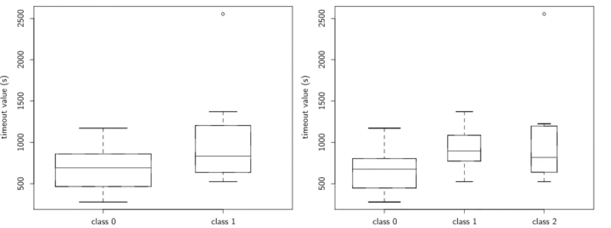
. ... ... ... ... ... . . . . . . . . . . . . . . . . . . . . . . . . . . . . . . . . . . . . . . . . . . . . . . . . . . . . . . . . . . . . . . . . . . . . . . . . . . . . . . . . . . . . . . . . . . . . . . . . . . . . . . . . . . . . . . . . . . . . . . . . . . . . . . . . . . . . . . . . . . . . . . . . . . . . . . . . . . . . . . . . . . . . . . . . . . . . . . . . . . . . . . . . . . . . . . . . . . . . . . . . . . . . . . . . . . . . . . . . . . . . . . . . . ... . . . . . . . . . . . . . . . . . . . . . . . . . . . . . . . . . . . . . . . . . . . . . . . . . . . . . . . . . . . . . . . . . . . . . . ... ... ... ... . ... . . . . . . . . . . . . . . . . . . . . . . . . . . . . . . . . . . . . . . . . . . . . . . . . . . . . . . . . . . . . . . . . . . . . . . . . . . . . . . . . . . . . . . . . . . . . . . . ... ... ... . . . . . . . . . . . . . . . . . . . . . . . . . . . . . . . . . . . . . . . . . . . . . . . . . . . . . . . . . . . . . . . . . . . . . . . . . . . . . . . . . . . . . . . . . . . . . . . . . . . . . . . . . . . . . . . . . . . . . . . . . . . . . . . . . . . . . . . . . . . . . . . . . . . . . . . . . . . . . . . . . . . . . . . . . . . . . . . . . . . . . . . . . . . . . . . . . . . . . . ... . . . . . . . . . . . . . . . . . . . . . . . . . . . . . . . . . . . . . . . . . . ... . . ... . . ... . . ... . ... . . . . . . . . . . . . . . . . . . . . . . . . . . . . . . . . . . . . . . . . . . . . . . . . . . . . . . . . . . . . . . . . . . . . . . . . . . . . . . . . . . . . . . . . . . . . . . . . . . . . . . . . . . . . . . . . . . . . . . . . . . . . . . . . . . . . . . . . . . . . . . . . ... . ... . . . . . . . . . . . . . . . . . . . . . . class 0 class 1 . . . . . . . . . . . . . . . . . . . . . . . . . . . . . . . . . . . . . . . . . . . . . . . . . . . . . . . . . . . . . . . . . . . . . . . . . . . . . . . . . . . . . . . . . . . . . . . . . . . . . . . . . . . . . . . . . . . . . . . . . . . . . . . . . . . . . . . . . . . . . . . . . . . . . . . . . . . . . . . . . . . . . . . . . . . . . . . . . . . . . . . . . . . . . . . . . . . . . . . . . . . . . . . . . . . . . . . . . . . . . . . . . . . . . . . . . . . . . . . . . . . . . . . . . . . . . . . . . . . . . . . . . . . . . . . . . . . . . . . . . . . . . . . . . . . . . . . . . . . . . . . . . . . . . . . . . . . . . . . . . . . . . . . . . . . . . . . . . . . . . . . . . . . . . . . . . . . . . . . . . . . . . . . . . . . . . . . . . . . . . . . . . . . . . . . . . . . . . . . . . . . . . . . . . . . . . . . . . . . . . . . . . . . . . . . . . . . . . . . . . . . . . . . . . . . . . . . . . . . . . . . . . . . . . . . . . . . . . . . . . . . . . . . . . . . . . . . . . . . . . . . . . . . . . . . . . . . . . . . . . . 5 0 0 1 0 0 0 1 5 0 0 2 0 0 0 2 5 0 0 ti m eo u t va lu e (s ) . . ... . . . . . . . . . . . . . . . . . . . . . . . . . . . . . . . . . . . . . . . . . . . . . . . . . . . . . . . . . . . . . . . . . . . . . . . . . . . . . . . . . . . . . . . . . . . . . . . . . . . . . . . . . . . . . . . . . . . . . . . . . . . . . . . . . . . . . . . . . . . . . . . . . . . . . . . . . . . . . . . . . . . . . . . . . . . . . . . . . . . . . . . . . . . . . . . . . . . . . . . . . . . . . . . . . . . . . . . . . . . . . . . . . . . . . . . . . . . . . . . . . . . . . . . . . . . . . . . . . . . . . . . . . . . . . . . . . . . . . . . . . . . . . . . . . . . . . . . . . . . . . . . . . . . . . . . . . . . . . . . . . . . . . . . . . . . . . . . . . . . . . . . . . . . . . . . . . . . . . . . . . . . . . . . . . . . . . . . . . . . . . . . . . . . . . . . . . . . . . . . . . . . . . . . . . . . . . . . . . . . . . . . . . . . . . . . . . . . . . . . . . . . . . . . . . . . . . . . . . . . . . . . . . . . . . . . . . . . . . . . . . . . . . . . . . . . . . . . . . . . . . . . . . . . . . . . . . . . . . . . . . . . . . . . . . . . . . . . . . . . . . . . . . . . . . . . . . . . . . . . . . . . . . . . . . . . . . . . . ... ... ... . . . . . . . . . . . . . . . . . . . . . . . . . . . . . . . . . . . . . . . . . . . . . . . . . . . . . . . . . . . . . . . . . . . . . . . . . . . . . . . . . . . . . . . . . . . . . . . . . . . . . . . . . . . . . . . . . . . . . . . . . . . . . . . . . . . . . . . . . . . . . . . . . . . . . . . . . . . . . . . . . . ... . . . . . . . . . . . . . . . . . . . . . . . . . . . . . . . . . . . . . . . . . . . . . . . . . . . . . . . . . . . . . . . . . . . . . . . . . . . ... . . ... . . ... . . ... . . ... . . ... . ... . . . . . . . . . . . . . . . . . . . . . . . . . . . . . . . . . . . . . . . . . . . . . . . . . . . . . . . . . . . . . . . . . . . . . . . . . . . . . . . . . . . . . ... ... . . . . . . . . . . . . . . . . . . . . . . . . . . . . . . . . . . . . . . . . . . . . . . . . . . . . . . . . . . . . . . . . . . . . . . . . . . . . . . . . . . . . . . . . . . . . . . . ... . . . . . . . . . . . . . . . . . . . . . . . . . . . . . . . . . . . . . . . . . . . . . . . . . . . . . . . . . . . . . . . . . . . . . . . . . ... ... ... ... ... ... ... . . . . . . . . . . . . . . . . . . . . . . . . . . . . . . . . . . . . . . . . . . . . . . . . . . . . . . . . . . . . . . . . . . . . . . . . . . . . ... ... . . . . . . . . . . . . . . . . . . . . . . . . . . . . . . . . . . . . . . . . . . . . . . . . . . . . . . . . . . . . . . . . . . . . . . . . . . . . . . . . . . . . . . . . . . . . . . . . . . . . . . . . . . . . . . . . . . . . . . . . . . . . . . . . . . . . . . . . . . . . . . . . . . . . . . . . . ... . . . . . . . . . . . . . . . . . . . . . . . . . . ... ... ... ... ... ... . ... . . . . . . . . . . . . . . . . . . . . . . . . . . . . . . . . . . . . . . . . . . . . . . . . . . . . . . . . . . . . . . . . . . . . . . . . . . . . . . . . . . . . . . . . . . . . . . . . . . . . . . . . . . . . . . . . . . . . . . . . . . . . . . . . . . . . . . . . . . . . . ... ... . . . . . . . . . . . . . . . . . . . . . . . . . . . . . . . . . class 0 class 1 class 2 . . . . . . . . . . . . . . . . . . . . . . . . . . . . . . . . . . . . . . . . . . . . . . . . . . . . . . . . . . . . . . . . . . . . . . . . . . . . . . . . . . . . . . . . . . . . . . . . . . . . . . . . . . . . . . . . . . . . . . . . . . . . . . . . . . . . . . . . . . . . . . . . . . . . . . . . . . . . . . . . . . . . . . . . . . . . . . . . . . . . . . . . . . . . . . . . . . . . . . . . . . . . . . . . . . . . . . . . . . . . . . . . . . . . . . . . . . . . . . . . . . . . . . . . . . . . . . . . . . . . . . . . . . . . . . . . . . . . . . . . . . . . . . . . . . . . . . . . . . . . . . . . . . . . . . . . . . . . . . . . . . . . . . . . . . . . . . . . . . . . . . . . . . . . . . . . . . . . . . . . . . . . . . . . . . . . . . . . . . . . . . . . . . . . . . . . . . . . . . . . . . . . . . . . . . . . . . . . . . . . . . . . . . . . . . . . . . . . . . . . . . . . . . . . . . . . . . . . . . . . . . . . . . . . . . . . . . . . . . . . . . . . . . . . . . . . . . . . . . . . . . . . . . . . . . . . . . . . . . . . . . 5 0 0 1 0 0 0 1 5 0 0 2 0 0 0 2 5 0 0 ti m eo u t va lu e (s ) . . ... . . . . . . . . . . . . . . . . . . . . . . . . . . . . . . . . . . . . . . . . . . . . . . . . . . . . . . . . . . . . . . . . . . . . . . . . . . . . . . . . . . . . . . . . . . . . . . . . . . . . . . . . . . . . . . . . . . . . . . . . . . . . . . . . . . . . . . . . . . . . . . . . . . . . . . . . . . . . . . . . . . . . . . . . . . . . . . . . . . . . . . . . . . . . . . . . . . . . . . . . . . . . . . . . . . . . . . . . . . . . . . . . . . . . . . . . . . . . . . . . . . . . . . . . . . . . . . . . . . . . . . . . . . . . . . . . . . . . . . . . . . . . . . . . . . . . . . . . . . . . . . . . . . . . . . . . . . . . . . . . . . . . . . . . . . . . . . . . . . . . . . . . . . . . . . . . . . . . . . . . . . . . . . . . . . . . . . . . . . . . . . . . . . . . . . . . . . . . . . . . . . . . . . . . . . . . . . . . . . . . . . . . . . . . . . . . . . . . . . . . . . . . . . . . . . . . . . . . . . . . . . . . . . . . . . . . . . . . . . . . . . . . . . . . . . . . . . . . . . . . . . . . . . . . . . . . . . . . . . . . . . . . . . . . . . . . . . . . . . . . . . . . . . . . . . . . . . . . . . . . . . . . . . . . . . . . . . . .
Fig. 10. Timeout values repartition after k-mean classification into 2 classes (left) and 3 classes (right) of CE-queues.
7.2.3 Testing different number of classes for CE-queues
Different aggregations of CE-queues were tested based on their cdf using the k-means classification algorithm with k = 2 to 10 classes. For each CE-queue,
the optimal timeout value is computed by minimizing equation 1. Figure 10
shows the repartition of the timeout values in the classes. The width of each box is proportional to the number of CE-queues in the class.
In order to measure if the classes are statistically discriminant, we have tested
the hypothesis H0“all sets have equal mean and equal variance” using ANOVA.
The results are reported in the following table where Df corresponds to the number of degrees of freedom, F to the ratio statistic of the between groups variance to the within groups variance and p value to the significance level of
H0. Symbol *** means rejection of hypothesis H0 with high confidence (level
1% of p < 0.01).
nb. of classes Df F p value H0 rejection
2 1 13.9 4.10−04 *** 3 2 10.0 1.10−04 *** 4 3 14.1 2.10−07 *** 5 4 10.3 1.10−06 *** 6 5 8.4 2.10−06 *** 7 6 10.9 1.10−08 *** 8 7 9.6 2.10−08 *** 9 8 9.5 8.10−09 *** 10 9 8.3 3.10−08 ***
... ... ... ... ... . . . . . . . . . . . . . . . . . . . . . . . . . . . . . . . . . . . . . . . . . . . . . . . . . . . . . . . . . . . . . . . . . . . . . . . . . . . . . . . . . . . . . . . . . . . . . . . . . . . . . . . . . . . . . . . . . . . . . . . . . . . . . . . . . . . . . . . . . . . . . . . . . . . . . . . . . . . . . . . . . . . . . . . . . . . . . . . . . . . . . . . . . . . . . . . . . . . . . . . . . . . . . . ... . . . . . . . . . . . . . . . . . . . . . . . . . . . . . . . . . . . . . . . . . . . . . . . . . . . . . . . . . . . . . . . . . . . . . . . . . . ... . ... . ... . ... ... . . . . . . . . . . . . . . . . . . . . . . . . . . . . . . . . . . . . . . . . . . . . . . . . . . . . . . . . . . . . . . . . . . . . . . . . . . . . . . . . . . . . ... ... ... . . . . . . . . . . . . . . . . . . . . . . . . . . . . . . . . . . . . . . . . . . . . . . . . . . . . . . . . . . . . . . . . . . . . . . . . . . . . . . . . . . . . . . . . . . . . . . . . . . . . . . . . . . . . . . . . . . . . . . . . . . . . . . . . . . . . . . . . . . . . . . . . . . . . . . . . . . . . . . . . . . . . . . . . . . . . . . . . . . . . . . . . . . . . . . . . . . . . . . . . . . . . . . . . . . ... . . . . . . . . . . . . . . . . . . . . . . . . . . . . . . . . . . . . . . . . . . . . . . . . . . . . . . . . . ... . . ... . . ... . . ... ... . . . . . . . . . . . . . . . . . . . . . . . . . . . . . . . . . . . . . . . . . . . . . . . . . . . . . . . . . . . . . . . . . . . . . . . . . . . . . . . . . . . . . . . . . . . . . . . . . . . . . . . . . . . . . . . . . . . . . . . ... . . ... . . . . . . . . . . . . . . . . . . . . . . class 0 class 1 2 . . . . . . . . . . . . . . . . . . . . . . . . . . . . . . . . . . . . . . . . . . . . . . . . . . . . . . . . . . . . . . . . . . . . . . . . . . . . . . . . . . . . . . . . . . . . . . . . . . . . . . . . . . . . . . . . . . . . . . . . . . . . . . . . . . . . . . . . . . . . . . . . . . . . . . . . . . . . . . . . . . . . . . . . . . . . . . . . . . . . . . . . . . . . . . . . . . . . . . . . . . . . . . . . . . . . . . . . . . . . . . . . . . . . . . . . . . . . . . . . . . . . . . . . . . . . . . . . . . . . . . . . . . . . . . . . . . . . . . . . . . . . . . . . . . . . . . . . . . . . . . . . . . . . . . . . . . . . . . . . . . . . . . . . . . . . . . . . . . . . . . . . . . . . . . . . . . . . . . . . . . . . . . . . . . . . . . . . . . . . . . . . . . . . . . . . . . . . . . . . . . . . . . . . . . . . . . . . . . . . . . . . . . . . . . . . . . . . . . . . . . . . . . . . . . . . . . . . . . . . . . . . . . . . . . . . . . . . . . . . . . . . . . . . . . . . . . . . . . . . . . . . . . . . . . . . . . . . . . . . . . 5 0 0 1 0 0 0 1 5 0 0 2 0 0 0 2 5 0 0 classes ti m eo u t va lu e (s ) . . ... . . . . . . . . . . . . . . . . . . . . . . . . . . . . . . . . . . . . . . . . . . . . . . . . . . . . . . . . . . . . . . . . . . . . . . . . . . . . . . . . . . . . . . . . . . . . . . . . . . . . . . . . . . . . . . . . . . . . . . . . . . . . . . . . . . . . . . . . . . . . . . . . . . . . . . . . . . . . . . . . . . . . . . . . . . . . . . . . . . . . . . . . . . . . . . . . . . . . . . . . . . . . . . . . . . . . . . . . . . . . . . . . . . . . . . . . . . . . . . . . . . . . . . . . . . . . . . . . . . . . . . . . . . . . . . . . . . . . . . . . . . . . . . . . . . . . . . . . . . . . . . . . . . . . . . . . . . . . . . . . . . . . . . . . . . . . . . . . . . . . . . . . . . . . . . . . . . . . . . . . . . . . . . . . . . . . . . . . . . . . . . . . . . . . . . . . . . . . . . . . . . . . . . . . . . . . . . . . . . . . . . . . . . . . . . . . . . . . . . . . . . . . . . . . . . . . . . . . . . . . . . . . . . . . . . . . . . . . . . . . . . . . . . . . . . . . . . . . . . . . . . . . . . . . . . . . . . . . . . . . . . . . . . . . . . . . . . . . . . . . . . . . . . . . . . . . . . . . . . . . . . . . . . . . . . . . . . . .
Fig. 11. k-means classification into 3 classes after grouping classes 1 and 2.
The result of the ANOVA test shows that the H0 hypothesis is strongly
re-jected in all cases at a level less than 1% (between 8.10−7
% and 0.04 %). The best result is obtained for 9 classes but the gain is not so high. Note that
the ANOVA test only shows that the hypothesis H0 is rejected: this does not
necessary imply that all classes differ from each other.
In the case of 2 classes, these classes are statistically discriminant. But for more than 2 classes, further tests must be done in order to determine how many classes are independent.
7.2.4 Refining the ANOVA analysis
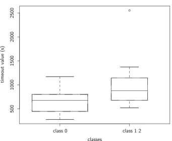
For example, let us look at the case of classification into 3 different classes (classes 0, 1 and 2). Using ANOVA, if we test classes 1 and 2, we observe that they do not differ significantly: F = 0.2334 (p = 0.6338). Building a new class (class 1+2) from classes 1 and 2, we now test class 0 against class 1+2 and obtain that they differ significantly: F = 19.651 (p = 3.003e − 05). We observe that grouping two classes after the classification k = 3 gives a similar, although slightly better, result than the classification k = 2.
The optimal timeout for the 2 populations (classes 0 and 1+2) are t∞0 = 779s
and t∞1+2 = 881s respectively leading to an optimal execution time of EJ =
398s and EJ = 794s respectively (see figure 12).
optimal t∞ min EJ EJ(t∞ref) ∆%
all data t∞ref = 556s 479s
class 0 730s 398s 399s 0.2%
0 0.2 0.4
cumulative density function FR
0.6 0.8 1 0 2000 4000 latency (s) 6000 8000 10000 "class 0" "class 1+2" "whole class 0" "whole class 1+2"
Fig. 12. Cumulative density functions of latency with respect to time (in seconds). This figure is obtained from the k-means classification into 3 classes. We grouped the last 2 classes into a single one so that we have 2 classes: the initial class 0 (in red) and new class 1+2 (in green) resulting of the merging of classes 1 and 2. Each curve corresponds to the cdf of one CE-queue. The blue and magenta curves correspond to the cdf of the centroid of class 0 and class 1+2 respectively.
... ... ... . . . . . . . . . . . . . . . . . . . . . . . . . . . . . . . . . . . . . . . . . . . . . . . . . . . . . . . . . . . . . . . . . . . . . . . . . . . . . . . . . . . . . . . . . . . . . . . . . . . . . . . . . . . . . . . . . . . . . . . . . . . . . . . . . . . . . . . . . . . . . . . . . . . . . . . . . . . . . . . . . . . . . . . . . . . . . . . . . . . . . . . . . . . . ... . . . . . . . . . . . . . . . . . . . . . . . . . . . . . . . . . . . . . . . . . . . . . . . . . . . . . . . . . . . . . . . . . . . . . . . . . . . . . . . . . . . . . . . ... ... ... ... ... . . . . . . . . . . . . . . . . . . . . . . . . . . . . . . . . . . . . . . . . . . . . . . . . . . . . . . . . . . . . . . . . . . . . . . . . . . . . . . . . . . . . . . . . . . . . . . . . . . . . . . . . . . . . ... ... ... ... ... ... . . . . . . . . . . . . . ... . . . . . . . . . . . . . . . ... . ... . ... . ... ... . . . . . . . . . . . . . . . . . . . . . . . ... . . . . . . . . . ... . . . . . . . . . ... . . . . . . . . . ... . . . . . . ... . . . . . . . . . ... . . ... . . . . . . . . . . . . . . . . . . . . . . class 0 class 1 2 . . . . . . . . . . . . . . . . . . . . . . . . . . . . . . . . . . . . . . . . . . . . . . . . . . . . . . . . . . . . . . . . . . . . . . . . . . . . . . . . . . . . . . . . . . . . . . . . . . . . . . . . . . . . . . . . . . . . . . . . . . . . . . . . . . . . . . . . . . . . . . . . . . . . . . . . . . . . . . . . . . . . . . . . . . . . . . . . . . . . . . . . . . . . . . . . . . . . . . . . . . . . . . . . . . . . . . . . . . . . . . . . . . . . . . . . . . . . . . . . . . . . . . . . . . . . . . . . . . . . . . . . . . . . . . . . . . . . . . . . . . . . . . . . . . . . . . . . . . . . . . . . . . . . . . . . . . . . . . . . . . . . . . . . . . . . . . . . . . . . . . . . . . . . . . . . . . . . . . . . . . . . . . . . . . . . . . . . . . . . . . . . . . . . . . . . . . . . . . . . . . . . . . . . . . . . . . . . . . . . . . . . . . . . . . . . . . . . . . . . . . . . . . . . . . . . . . . . . . . . . . . . . . . . . . . . . . . . . . . . . . . . . . . . . . . . . . . . . . . . . . . . . . . . . . . . . . . . . . . . . . . . . . . . . . . . . . . . . . . . . . . . . . . . . . . . . . . . . . . . . . . . . . . . . . . . . . . . 0 1 0 0 2 0 0 3 0 0 4 0 0 classes er ro r (s ) . . ... . . . . . . . . . . . . . . . . . . . . . . . . . . . . . . . . . . . . . . . . . . . . . . . . . . . . . . . . . . . . . . . . . . . . . . . . . . . . . . . . . . . . . . . . . . . . . . . . . . . . . . . . . . . . . . . . . . . . . . . . . . . . . . . . . . . . . . . . . . . . . . . . . . . . . . . . . . . . . . . . . . . . . . . . . . . . . . . . . . . . . . . . . . . . . . . . . . . . . . . . . . . . . . . . . . . . . . . . . . . . . . . . . . . . . . . . . . . . . . . . . . . . . . . . . . . . . . . . . . . . . . . . . . . . . . . . . . . . . . . . . . . . . . . . . . . . . . . . . . . . . . . . . . . . . . . . . . . . . . . . . . . . . . . . . . . . . . . . . . . . . . . . . . . . . . . . . . . . . . . . . . . . . . . . . . . . . . . . . . . . . . . . . . . . . . . . . . . . . . . . . . . . . . . . . . . . . . . . . . . . . . . . . . . . . . . . . . . . . . . . . . . . . . . . . . . . . . . . . . . . . . . . . . . . . . . . . . . . . . . . . . . . . . . . . . . . . . . . . . . . . . . . . . . . . . . . . . . . . . . . . . . . . . . . . . . . . . . . . . . . . . . . . . . . . . . . . . . . . . . . . . . . . . . . . . . . . . . .
Fig. 13. Errors measured between minimal EJ and EJ(t∞ref), where t∞ref if
com-puted from all classes.
Figure13shows the errors computed between the minimal EJ and EJ(t∞ref),
where t∞ref is computed from all classes. It quantifies the performance loss
that can be expected when CE cdfs are approximated by the centroid of their class.
7.2.5 Discussion
The order of magnitude of the grid latency thus appears to be correlated to the execution CE-queue. It is not surprising because the CE is directly related to the job queuing time as a CE-queue exactly corresponds to a batch queue. Variations of middleware, system versions and availability of the site to VOs may explain the differences observed among the 2 different classes while vari-ations inside a given class may be coming from the load imposed by the users and the performance of CEs host hardware. However, in general, the execu-tion CE-queue is only known after the job submission, during the scheduling procedure. Thus, this information could only be exploited for parameters that can be updated once the job has been submitted, as for instance the timeout value or the application completion prediction, whereas parameters such as the granularity of the tasks to submit could not benefit from the CE-queue information.
We have seen previously in the paper that the influence of the RB is very low. It could be explained by the fact that RBs are connected to overlapped sets of CEs that may belong to different classes, thus merging the different behaviors we can see when considering the CEs.
400 450 500 550 600 650 700 750 800 0 200 400 600 800 1000
expectation of execution time EJ (s)
timeout values (s) Monday Tuesday Wednesday Thursday Friday Saturday Sunday week only week-end all days
Fig. 14. Expectation of job execution time for each day of the week.
7.3 Day of the week
Considering that the load of the grid may depend on human activity (users often start submitting jobs during working hours), we have, as a first step, con-sidered the influence of the day of the week on the latency. We expect different behaviors during week days and weekends, considering that in most western countries, Saturdays and Sundays are non working days. The considered data
set, presented in section 5, concerns several weeks.
Figure14shows the latency expectation for each day of the week. The different
days of week show different behaviors. However, there is no clear distinction between week and week-end. The two extrema curve correspond to Wednesday and Friday. An explanation is that on Fridays users might initiate experiments that will run over the weekend, thus creating a stress effect on Friday’s load. To quantify the influence of the day of the week, we compute, for each week
and each day of the week, the optimal timeout value, according to equation1.
These values are plotted on figure 15with respect to the day of the week. As
confirmed by ANOVA analysis, there is no significant difference between the days of the week (p = 0.5268).
We also present on figure 16the evolution of the optimal timeout value with
respect to the week of the experiment, for each day of the week. There is no evidence of absolute pertinence of the day of the week in this figure. Even the period between Christmas and New Year’s Eve is not really separated from
the others. However, in figure 17, we observe that, in most weeks, there is a
decrease of the best timeout value between Tuesday or Wednesday and Thurs-day followed by an increase until FriThurs-day or SaturThurs-day. This profile information needs further investigation to be exploited.
Fig. 15. For each day of the week and for each week, the best timeout value is computed. We have plotted boxes for each day of the week. According to ANOVA, there is no significant difference between the days of the week (p = 0.5268).
200 250 300 350 400 450 500 550 600 650 700 750 36 37 38 39 50 51 52 53 00 01 02 03
best timeout value (s)
week number "Monday" "Tuesday" "Wednesday" "Thursday" "Friday" "Saturday" "Sunday"
Fig. 16. Each curve corresponds to a day of the week. We plotted optimal timeout values with respect to the weeks of the experiment.
200 250 300 350 400 450 500 550 600 650 700 750
Mon Tue Wed Thu Fri Sat Sun
best timeout value (s)
day of the week "2007-36" "2007-37" "2007-38" "2007-39" "2007-50" "2007-51" "2007-52" "2007-53" "2008-00" "2008-01" "2008-02" "2008-03"
Fig. 17. Each curve corresponds to a week of the experiment. The optimal timeout value is plotted with respect to the day of the week.
100 200 300 400 500 600 700 0-4 am 4-8 am 8-12 am 0-4 pm 4-8 pm 8-12 pm
optimal timeout value (s)
time period of the day
"Monday" "Tuesday" "Wednesday" "Thursday" "Friday" "Saturday" "Sunday"
Fig. 18. Each curve corresponds to a day of the week. We plotted optimal timeout values with respect to the time period of the day. We observe that there is more variability for the night time periods than during the day.
This time context study will now be completed by the analysis of the hours in the day. Indeed, working and non-working periods may influence the sub-missions, and consequently the load on the grid and the latencies. As seen in this paragraph, the study of the day of the week is not convincing enough.
7.4 Hours of the day
In a first analysis, we divide days into periods of four hours: H0 (0-4 am), H1
(4-8 am), H2 (8-12 am), H3 (0-4 pm), H4 (4-8 pm) and H5 (8-12 pm),
We also select data using CEs from a similar timezone: Austria, Belgium, Denmark, France, Germany, Italy, Netherlands, Portugal, Spain and Sweden (565 measures from week 7 to week 10).
For each day of the week, and for each time period of the day, we have
com-puted the latency cdf FR and the optimal timeout value that is displayed on
figure 18.
Moreover, figure 19plots the different population of latency for the different
hours of the week. We compare the results using (i) all CEs and all days, (ii) only CEs from the same timezone and all days and (iii) only CEs from the same timezone and only working days (Monday to Friday). An ANOVA on all those analysis confirms that the population of jobs submitted during a same one hour period are all statistically identical (p = 0.57 in case of all CEs,
p= 0.35 in case of one timezone and p = 0.12 with only working days).
Even if the ANOVA score is lower when using only one timezone and working days, the populations are still statistically equivalent: the time parameter has
an influence but too small to be statistically relevant.
Furthermore, we have separated data from working periods during weekdays and weekends as follows:
working period : Monday to Friday, 8am to 6pm
non-working period : Monday to Friday, 6pm to 8am, whole Saturday and Sunday
We then computed the optimal value for all the data, considering supposed working periods and supposed non working periods. As shown in this table, it does not lead to any better distinction between time periods.
data set optimal t∞ min EJ EJ(t∞ref) ∆EJ
all data t∞ref = 429s 451.5s
working period 476s 448.4s 449.1s 0.3%
non-working period 429s 452.6s 452.6s 0%
As a partial conclusion of this time period study, its influence is very small as compared to the variations of the model parameter along time and the classes of CEs. Other works have shown that the time parameter influence
parameters of the grid, such as [NPF08]. However, they have done their study
on a national grid with users in the same country. In our case, even if we choose CEs from the same timezone, many RB worldwide are connected to these CEs, and people all around the world will use these RBs. The EGEE grid is permanently used and no significant load pattern changes can be correlated to working periods.
8 Conclusion
From the work presented in this paper, we can extract two guidelines for job monitoring:
• Due to variations of the load conditions over long periods of time, timeout
optimization (equation 1) may benefit from updates along time (as for
ex-ample, once a week). Future work will focus on strategies to perform this update.
• Some context parameters related to the EGEE production grid such as CE-queues have an influence on the expected job execution time. Moreover, we have shown that we can group CE-queues into classes that are statistically
different, thus reducing the number of data to be analyzed4. Practically,
this means that timeout values (t∞) can be adapted depending on the class
of the CE where a job is scheduled.
The experiments on the influence of the RB or the time period (both day of the week and hour of the day) show that even if the influence on optimal timeout values is significant, it has a hardly relevant impact on the final expected execution time. An optimistic explanation could be that the EGEE production grid is used almost continuously by people around the world without noticeable time patterns and that RBs are roughly equivalent.
Future works will study other submission strategies than the one explained in
section 4. Studying other parameters such as specific job requirements that
constrain the execution targets is also planned.
9 Acknowledgements
This work is partially funded by the French national research agency (ANR),
NeuroLOG project5 under contract number ANR-06-TLOG-024. This project
is in the scope of scientific topics of the STIC-ASIA OnCoMedia project6. We
are grateful to the EGEE European project for providing the grid infrastruc-ture and user assistance.
References
[ABEHG08] Gabriel Aparicio, Ignacio Blanquer Espert, and Vicente Hern-ndez Garca. A Highly Optimized Grid Deployment: the
Metage-nomic Analysis Example. In Global Healthgrid: e-Science
Meets Biomedical INformatics (Healthgrid’08), pages 105 –115,
Chicago, USA, May 2008. Healthgrid, IOS Press.
[CD06] Eddy Caron and Fr´ed´eric Desprez. DIET: A Scalable Toolbox to
Build Network Enabled Servers on the Grid. International
Jour-nal of High Performance Computing Applications, 20(3):335–352,
2006.
[CGV08] Konstantinos Christodoulopoulos, Vasileios Gkamas, and
Em-manouel A. Varvarigos. Statistical Analysis and Modeling of 4 The methodology used could be applied to other grids by replacing CEs and RBs
by the equivalent workload management services. In the DIET middleware [CD06] for instance, it could correspond to Master Agents (MA) and Local Agents (LA).
5 NeuroLog: http://neurolog.polytech.unice.fr 6 OnCoMedia: http://www.onco-media.com
Jobs in a Grid Environment. Journal of Grid Computing (JGC), 6(1), March 2008.
[DCDO07] Georges Da Costa, Marios D. Dikaiakos, and Salvatore Orlando.
Nine months in the life of EGEE: a look from the South. In IEEE
International Symposium on Modeling, Analysis, and Simulation of Computer and Telecommunication Systems (MASCOTS’07),
pages 281–287, Istanbul, Turkey, October 2007. IEEE.
[Fei02] Dror Feitelson. Workload modeling for performance evaluation,
pages 114–141. Springer-Verlag - LNCS vol 2459, September 2002.
[Fis25] Ronald A. Fisher. Statistical Methods for Research Workers.
Oliver and Boyd, 1925.
[GLMR07] Tristan Glatard, Diane Lingrand, Johan Montagnat, and Michel
Riveill. Impact of the execution context on Grid job perfor-mances. In International Workshop on Context-Awareness and
Mobility in Grid Computing (WCAMG’07) (CCGrid’07), pages
713–718, Rio de Janeiro, May 2007. IEEE.
[GLMT08] C´ecile Germain, Charles Loomis, Jakub T. Mo´scicki, and
Ro-main Texier. Scheduling for Responsive Grids. Journal of Grid
Computing (JGC), 6(1):15–27, March 2008.
[GMP06] Tristan Glatard, Johan Montagnat, and Xavier Pennec.
Proba-bilistic and dynamic optimization of job partitioning on a grid infrastructure. In 14th euromicro conference on Parallel,
Dis-tributed and network-based Processing (PDP06), pages 231–238,
Montbliard-Sochaux, France, February 2006.
[GMP07] Tristan Glatard, Johan Montagnat, and Xavier Pennec.
Opti-mizing jobs timeouts on clusters and production grids. In
Inter-national Symposium on Cluster Computing and the Grid (CC-Grid’07), pages 100–107, Rio de Janeiro, May 2007. IEEE.
[GMP08] Tristan Glatard, Johan Montagnat, and Xavier Pennec. A
prob-abilistic model to analyse workflow performance on production
grids. In Priol et al. [PLB08], pages 510–517.
[ILJ+08] Alexandru Iosup, Hui Li, Mathieu Jan, Shanny Anoep, Catalin
Dumitrescu, Lex Wolters, and Dick Epema. The Grid Workloads Archive. Future Generation Computer Systems, 24(7):672–686, July 2008.
[LGW04] Hui Li, David Groep, and Lex Walters. Workload Characteristics
of a Multi-cluster Supercomputer. In Job Scheduling Strategies
for Parallel Processing, pages 176–193. Springer Verlag, 2004.
[LMG08] Diane Lingrand, Johan Montagnat, and Tristan Glatard.
Es-timating the execution context for refining submission strate-gies on production grids. In Assessing Models of Networks and
Distributed Computing Platforms (ASSESS / ModernBio) (CC-grid’08), pages 753 – 758, Lyon, May 2008. IEEE.
Workflow Execution in the Grid. IEEE Transactions on Systems,
Man, and Cybernetics, 36(3), May 2006.
[NMB+06] Daniel Nurmi, Anirban Mandal, John Brevik, Chuck Koelbel,
Richard Wolski, and Ken Kennedy. Evaluation of a Workflow Scheduler Using Integrated Performance Modelling and Batch Queue Wait Time Prediction. In Conference on High
Perfor-mance Networking and Computing, Tampa, Florida, November
2006. ACM Press.
[NPF08] Farrukh Nadeem, Radu Prodan, and Thomas Fahringer.
Charac-terizing, Modeling and Predicting Dynamic Resource
Availabil-ity in a Large Scale Multi-Purpose Grid. In Priol et al. [PLB08],
pages 348–357.
[OCV07] Michael Oikonomakos, Kostas Christodoulopoulos, and
Em-manouel Varvarigos. Profiling Computation Jobs in Grid Sys-tems. In IEEE International Symposium on Cluster Computing
and the Grid (CCGrid07), pages 197–204, Rio de Janeiro, Brasil,
May 2007.
[PLB08] Thierry Priol, Laurent Lefevre, and Rajkumar Buyya, editors.
IEEE International Symposium on Cluster Computing and the Grid, Lyon, France, May 2008. IEEE.
[RBJS06] Sahobimaholy Ravelomanana, Silvia Cristina Sordela Bianchi,
Chibli Joumaa, and Michelle Sibilla. A Contextual GRID Mon-itoring by a Model Driven Approach. In Proceedings of the
Ad-vanced International Conference on Telecommuni cations and In-ternational Conference on Internet and Web Applications and Servic (AICT/ICIW), pages 37–43, Gosier, Guadeloupe,
Febru-ary 2006. IEEE.
[SB99] Jennifer Schopf and Francine Berman. Stochastic Scheduling. In
Supercomputing (SC’99), Portland, USA, 1999.
[Ste56] H. Steinhaus. Sur la division des corps mat´eriels en parties. Bull.
Acad. Polon. Sci., IV(C1.II):801–804, 1956.
[SW04] Martin Swany and Rich Wolski. Building Performance
Topolo-gies for Computational Grids. International Journal of High
Performance Computing and Applications (IJHPCA), 18(2):255–
265, May 2004.
A Proof of Equation 1.
Given that ρ is the ratio of outliers, t∞ the timeout value and FR the
cumu-lative density function latency R for non outliers jobs, we denote by q the probability for a job to timeout. A job timeout if it is an outlier or if it faces