HAL Id: hal-02652500
https://hal.inrae.fr/hal-02652500
Submitted on 29 May 2020
HAL is a multi-disciplinary open access
archive for the deposit and dissemination of
sci-entific research documents, whether they are
pub-lished or not. The documents may come from
teaching and research institutions in France or
abroad, or from public or private research centers.
L’archive ouverte pluridisciplinaire HAL, est
destinée au dépôt et à la diffusion de documents
scientifiques de niveau recherche, publiés ou non,
émanant des établissements d’enseignement et de
recherche français ou étrangers, des laboratoires
publics ou privés.
genome-wide association genetics and diversity patterns
reveal key genomic regions, with a major contribution of
the Vgt2 (ZCN8) locus
Sophie Bouchet, Bertrand Servin, Pascal Bertin, Delphine Madur, Valerie
Combes, Fabrice Dumas, Dominique Brunel, Jacques Laborde, Alain
Charcosset, Stephane Nicolas
To cite this version:
Sophie Bouchet, Bertrand Servin, Pascal Bertin, Delphine Madur, Valerie Combes, et al.. Adaptation
of maize to temperate climates: mid-density genome-wide association genetics and diversity patterns
reveal key genomic regions, with a major contribution of the Vgt2 (ZCN8) locus. PLoS ONE, Public
Library of Science, 2013, 8 (8), �10.1371/journal.pone.0071377�. �hal-02652500�
Genome-Wide Association Genetics and Diversity
Patterns Reveal Key Genomic Regions, with a Major
Contribution of the
Vgt2
(
ZCN8
) Locus
Sophie Bouchet1¤, Bertrand Servin2, Pascal Bertin1, Delphine Madur1, Vale´rie Combes1, Fabrice Dumas1, Dominique Brunel3, Jacques Laborde4, Alain Charcosset1*, Ste´phane Nicolas1
1 UMR de Ge´ne´tique Ve´ge´tale, INRA – Universite´ Paris-Sud – CNRS, Gif-sur-Yvette, France, 2 UMR444, Laboratoire de Genetique Cellulaire, INRA, Castanet-Tolosan, France, 3 UR1279, Etude du Polymorphisme des Ge´nomes Ve´ge´taux, INRA, Commissariat a` l’Energie Atomique (CEA) Institut de Ge´nomique, Centre National de Ge´notypage, Evry, France,4 INRA Stn Expt Mais, St Martin De Hinx, France
Abstract
The migration of maize from tropical to temperate climates was accompanied by a dramatic evolution in flowering time. To gain insight into the genetic architecture of this adaptive trait, we conducted a 50K SNP-based genome-wide association and diversity investigation on a panel of tropical and temperate American and European representatives. Eighteen genomic regions were associated with flowering time. The number of early alleles cumulated along these regions was highly correlated with flowering time. Polymorphism in the vicinity of the ZCN8 gene, which is the closest maize homologue to Arabidopsis major flowering time (FT) gene, had the strongest effect. This polymorphism is in the vicinity of the causal factor of Vgt2 QTL. Diversity was lower, whereas differentiation and LD were higher for associated loci compared to the rest of the genome, which is consistent with selection acting on flowering time during maize migration. Selection tests also revealed supplementary loci that were highly differentiated among groups and not associated with flowering time in our panel, whereas they were in other linkage-based studies. This suggests that allele fixation led to a lack of statistical power when structure and relatedness were taken into account in a linear mixed model. Complementary designs and analysis methods are necessary to unravel the architecture of complex traits. Based on linkage disequilibrium (LD) estimates corrected for population structure, we concluded that the number of SNPs genotyped should be at least doubled to capture all QTLs contributing to the genetic architecture of polygenic traits in this panel. These results show that maize flowering time is controlled by numerous QTLs of small additive effect and that strong polygenic selection occurred under cool climatic conditions. They should contribute to more efficient genomic predictions of flowering time and facilitate the dissemination of diverse maize genetic resources under a wide range of environments.
Citation: Bouchet S, Servin B, Bertin P, Madur D, Combes V, et al. (2013) Adaptation of Maize to Temperate Climates: Mid-Density Genome-Wide Association Genetics and Diversity Patterns Reveal Key Genomic Regions, with a Major Contribution of the Vgt2 (ZCN8) Locus. PLoS ONE 8(8): e71377. doi:10.1371/ journal.pone.0071377
Editor: James C. Nelson, Kansas State University, United States of America Received December 7, 2012; Accepted July 1, 2013; Published August 30, 2013
Copyright: ß 2013 Bouchet et al. This is an open-access article distributed under the terms of the Creative Commons Attribution License, which permits unrestricted use, distribution, and reproduction in any medium, provided the original author and source are credited.
Funding: Phenotyping experimentations were funded by INRA, Genoplante, and Gabi-Genoplante projects. Genotyping was funded by INRA and CornFed trilateral project (jointly funded by French ANR, German BMBF and Spanish MICINN). Sophie Bouchet was funded by ANR projects Hypermaize and CornFed. The funders had no role in study design, data collection and analysis, decision to publish, or preparation of the manuscript.
Competing Interests: The authors have declared that no competing interests exist. * E-mail: alain.charcosset@moulon.inra.fr
¤ Current address: Euralis, Domaine de Sandreau, Mondonville, France
Introduction
Maize was domesticated in tropical conditions in the lowlands of southwest Mexico and later adapted to the broadest range of
climatic conditions of all crops, from 40uS in Chile to 50uN in
Canada and Russia, from sea level in the West Indies to elevations above 3400 m in the Andes [1–4]. Maize has high molecular diversity, with landraces pooling most of the nucleotide diversity (83%) from their wild ancestors, contrary to many other species [1]. This illustrates that a limited bottleneck occurred during domestication [2–4], probably due to the landrace outcrossing mating system and the continuous gene flow between cultivated and wild Zea mays L. subspecies. Modern breeding seems to have had little impact on genome-wide diversity and mostly affected
genes that had already undergone selection during domestication [1,2].
Despite this limited loss of diversity, phenotypes have been dramatically modified by domestication, large-scale migration/ adaptation and selection cycles that gave rise to modern hybrids. In particular, flowering time evolved to adapt to short growing seasons, long days and low temperatures under temperate climates. Among the germplasm available, for maize landraces, the time from planting to the mature grain stage ranges from 2 to 11 months [3]. Silk emergence date (female flowering) varies by 32 days among the founder lines of thenested association mapping (NAM) population and by 28 days among the recombinant inbred lines derived from these parents [4].
Flowering time plays a key role in the acclimation of plants to different environments by integrating diverse environmental and endogenous signals that control the optimal moment for the transition from the vegetative to the reproductive phase. It allows the plant to avoid drought and thus kernel abortion, or to optimize the light interception period and yield for instance. The synchrony of male and female flowering is also an important adaptive trait in maize as high asynchrony can result in yield losses, especially in modern uniform varieties [5].
Compared to some other species like Arabidopsis [6] sorghum [7] and rice [8,9], for which natural variations at a limited number of genes have been shown to have a large effect, flowering time architecture in maize is more complex. Several tens of small effect QTLs have been detected [4,10]. This suggests that maize flowering involves a network of genes interacting in many signaling pathways. Among the loci that have been highlighted, the maize INDETERMINATE1 (ID1) gene is an important regulator of maize autonomous flowering that acts in leaves to mediate the expression of mobile signals that are hypothetical flowering hormones called florigens [11,12,13] which promote flowering at the shoot apical meristem. ZCN8 was found to be controlled by ID1 and to express a florigen in leaves [14]. It is homologous to the Arabidopsis FLOWERING LOCUS T (FT), a kinase regulator [15]. FT is a key integrator because almost all flowering pathways (autonomous, gibberellins, photoperiod and vernalization) converge on it, and FT transmits the floral inductive signal to downstream floral identity genes [16]. In maize, a family of 25 FT homologues including ZCN8 have been published [17]. They are named Zea CENTRORADIALIS (ZCN) genes. Expression analysis demonstrated that some of them are involved in developmental processes. A second gene that has been shown to have a major downstream effect is Dfl1 (Delayed flowering1), a transcription factor that expresses in the shoot apical region [18]. Mutants, however, exhibit a less severe flowering time defect compared to ID1. Another major factor in flowering time variation, Vgt1, was detected in both linkage-based QTL analyses and association genetics studies [4,10,19,20,21,22,23,24]. It has been cloned and described as a regulatory factor that controls the expression of an Apetala2-like gene, ZmRap2.7 [24].
Further investigations to identify the main factors controlling maize flowering time in a panel representative of diverse migration routes would be beneficial: (i) to gain insight into the adaptation mechanisms under changing environments, (ii) to identify alleles for introgression into existing varieties in order to adapt them to different environmental conditions, and (iii) to better predict flowering time to the benefit of global crop management and local breeding programs, since flowering time is often considered as a major covariate in yield estimation. This latter objective can presently be approached through genomic selection models. The choice of suitable models should consider the complexity of trait architectures in terms of relative individual effects of loci and possible existence of non-additive effects due to interaction with the genetic background (GxQ epistasis) or gene-environment interactions (GxE) [25,26,27]. In maize, neither Buckler et al. [4] nor Steinhoff et al. [28] identified major effects for GxQ or GxE interactions for photoperiod insensitive QTLs of flowering time. They concluded that a simple additive model can accurately predict flowering time, in contrast to the genetic architecture observed in the selfing plant species like rice and Arabidopsis. Steinhoff et al. [28], however observed some regions presenting epistatic interactions between chromosomes 4 and 8, and between chromosome 9 and chromosomes 2, 7 and 8, so these questions generally remain open.
High density genotyping tools available today are expected to help in the discovery, fine mapping and allele diversity character-ization of regions involved in flowering time. However, the choice of panel is very important as the level of polymorphism in each genetic group will determine the power of the analysis. In domesticated species like maize, loci that are critical to both local adaptation and yield performance, such as flowering time loci, are often targets of both natural and artificial selection, leading to complex forms of allele sharing and admixture among diverse genetic groups. Differentiation of flowering time between maize genetic groups is actually clear at the QTL level [29,30]. Genome-wide association mapping and selection scans can provide complementary information to help decipher the architecture of such adaptive traits. For example, in the case of extreme differentiation leading to fixation of different alleles in different groups, the loci will be undetectable when association genetics approaches are used that include structure in the model, but will show significant tests of selection.
This study was thus designed to assess the potential of currently available mid-density arrays [31] in order to gain further insight into the maize flowering time architecture. We analyzed a panel representing a broad range of lines adapted to different environments (tropical lines, Corn-Belt Dents and Stiff Stalk, Northern and European Flints) that has proven efficient in previous flowering time candidate gene-based association studies [21,30,32]. We therefore first compared the structure of the panel as obtained with different marker sets in order to use the most appropriate one for statistical analyses. In order to determine the extent and variation of LD [33] and to estimate the number of markers required to cover the genome for future exhaustive genome scans, we looked at LD using an unbiased measure that extracts the part of the correlation of allelic frequencies that is due to the intrinsic structure of the panel [34]. We then looked at diversity, LD patterns and selection signature along the genome. We conducted association studies focused on female (FFLW) and male flowering (MFLW) dates and anthesis-to-silking date intervals (ASI). The selection test and association study results were considered to identify key genomic regions involved in adaptation. We compared diversity and recombination patterns in flowering time QTLs compared to the rest of the genome in order to identify putative selective events that may have shaped flowering time along ancient migration routes.
Material and Methods Genetic materials
A sample of 375 maize lines representing the worldwide diversity was considered [30]. A conformity check of newly extracted DNA samples compared to reference DNA samples revealed 10 illegitimate or strongly divergent samples that were removed (see Data S1 in Text S1). Among the 365 remaining lines genotyped with the 50K Illumina array, 29 were removed since they had more than 10% missing data or 5% heterozygosity. Among the remaining 336 lines that presented good quality SSR and Illumina genotyping, the panel was composed of five genetic groups according to the STRUCTURE results obtained with 55 SSRs [30]. The respective contribution to each group was calculated as the sum of quantitative assignments of all lines to this group, which led to 57 Northern Flints (NF), 62 European Flints (EF), 26 Iowa Synthetic Stiff Stalks (SS), 115 Corn Belt Dents (CBD) and 76 tropical lines (Trop). Overall, 242 lines were assigned to one group (with a major contribution of .80%) and are further referred to as ‘‘non-admixed’’ lines. This sub-sample of
relatively non-admixed lines consisted of 30 NF, 39 EF, 9 SS, 109 CBD and 55 Trop (Table 1).
Molecular markers
The panel of maize lines was described using two different sets of SSR markers. The first one was described in [30]. It was composed of 54 tri-nucleotidic and 1 di-nucleotidic SSRs. The second one, reported here for the first time, consisted of 49 additional di-nucloetidic SSR markers. Di-nucleotidic SSRs have a higher mutation rate than tri-nucleotidic SSRs [35]. The panel was also genotyped with 57838 SNP markers synthesized for Illumina Golden Gate. Among them, 56110 (97%) markers passed the bead representation and decoding quality metrics, 49585 (88%) passed the analytical phase and could be scored with GenomeStudio v2009 software [31]. Then 45747 (92%) of these were polymorphic in the panel of 336 lines with less than 20% missing data and 15% heterozygosity and 45615 (99.7%) were not redundant according to the probe sequences. Among those, 43589 (95%) had a minor allele frequency (MAF) above 0.05. Finally 43224 (95% of polymorphic markers) non-redundant with MAF.0.05 were physically mapped on version 2 of the B73 genome sequence (called RefGen_v2) and were then used for linkage disequilibrium (LD) and association analyses. A subset of 29911 markers (65% of polymorphic markers, not always physically mapped) designed from 27 diverse founder lines called the Panzea diversity panel [36], non-redundant and potentially rare (MAF.0.01), were used for the diversity statistical calcula-tion. Most of the additional markers were designed for mapping in B736Mo17 populations [31]. They were considered for compu-tation of diversity indexes in comparison with Panzea SNP information and association genetics. Additional markers not belonging to these two main sets were from diverse origins and considered only for association genetics investigations.
As a reference, we considered 535 SNPs discovered on regions that were fully sequenced in the same panel around Vgt1 on chromosome 8 [21], ZmCCT on chromosome 10 [32] and Tb1-D8 on chromosome 1 [30] in order to compare the MAF distributions.
Similarity and Structure matrices
Similarity. We computed two different similarity matrices between lines (kinship), one considering the identity by state (IBS) with r-Emma [37] and the second considering the identity by
descent (IBD), estimated following [38], taking the allele frequency into account with Cocoa software [39]. These were applied to the three different sets of markers (55 SSRs, 94 SSRs and 29911 SNP Panzea markers). We compared the correlation between the three sets of markers, while removing the diagonals of the matrices.
Structure. Population structure was investigated in order to define suitable covariates for association genetics models and investigate genetic diversity trends among genetic groups. We thus used two different sets of SSR markers (55 SSRs and 94 SSRs) and STRUCTURE [40,41] software. We considered that lines were haploids and replaced heterozygous genotypes by missing data. We assumed a single domestication event and restricted our analysis to the correlated frequency model [41]. We set other parameters at their default values using the admixture model and
infer ALPHA option. We used a 104 burn-in period and 106
iterations. Allele frequencies in each of the K clusters (from 2 to 15) were estimated, and the percentage of genome derived from each cluster was estimated for each accession.
The structure matrix built with 29911 Panzea SNP markers was estimated by ADMIXTURE, which computes maximum likeli-hood estimations of individual ancestries from multilocus biallelic genotype datasets using the same statistical model as STRUC-TURE with a very fast numerical optimization algorithm [42].
Diversity levels revealed by the 50K Illumina array within and among genetic groups
Diversity parameters were estimated for the total panel and within each of the five main genetic groups determined from 55 SSRs [30], considering only 242 non-admixed lines (assigned to the different groups with a threshold of .0.8) and the set of 29911 Panzea markers. The minor allele frequency (MAF), observed
(HO), expected (HE) heterozygosity, differentiation (FST)
corre-sponding to the ratio of inter-group diversity over the total genetic diversity according to Nei [43,44] were calculated for each locus and overall loci at the group and panel levels. Bootstrap
confidence interval (over loci) for pairwise genetic group FST
[45] were calculated with one hundred permutations. All statistics were computed with r-Hierfstat [46].
Finally, we considered the classification based on 55 SSRs as a reference to estimate SNP allelic frequencies in each genetic group, as,
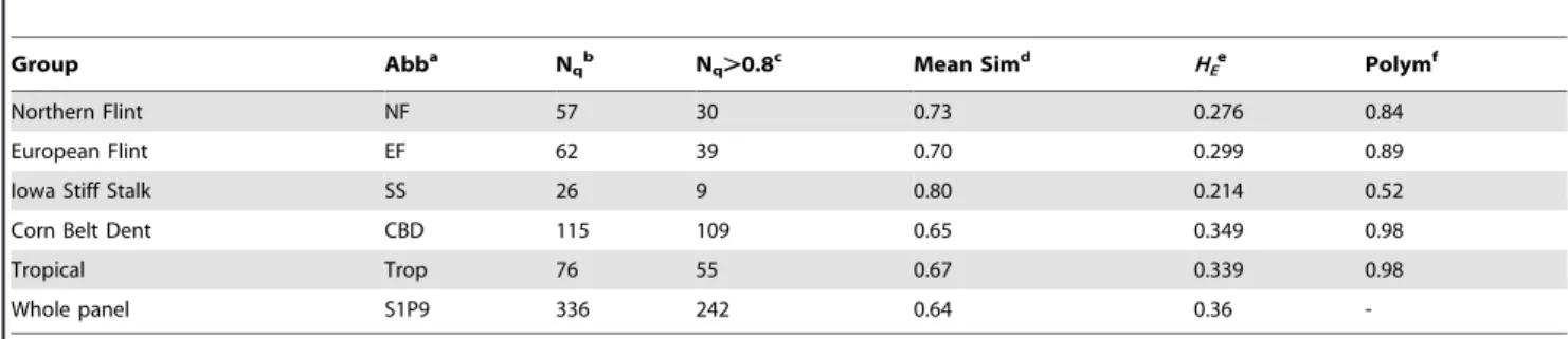
Table 1. Diversity statistics computed using 29911 Panzea SNP markers over the whole panel and five main genetic groups.
Group Abba
Nqb Nq.0.8c Mean Simd HEe Polymf
Northern Flint NF 57 30 0.73 0.276 0.84
European Flint EF 62 39 0.70 0.299 0.89
Iowa Stiff Stalk SS 26 9 0.80 0.214 0.52
Corn Belt Dent CBD 115 109 0.65 0.349 0.98
Tropical Trop 76 55 0.67 0.339 0.98
Whole panel S1P9 336 242 0.64 0.36
-a
Abb: abbreviation describing the group,
b
Nq=gidiqwith i the index of lines and q the index of groups, diqthe assignment proportion of line i to group q according to STRUCTURE software [40,41] using 55
SSRs, Nq the number of lines in group q;
c
number of lines assigned to group q with a genome proportion above 0.8;
d
mean similarity within each group, calculated with IBS (identity by state);
e
expected heterozygosity inside each group computed with r-Hierfstat [46]; f percentage of polymorphic loci within each group,
d,e,f
statistics were computed considering lines with assignment to one group above 0.8. doi:10.1371/journal.pone.0071377.t001
Pk(l)q~ X i diqXik(l)= X i diq
Where, Pk(l)qis the frequency of allele k at locus l in group q, diqis
the assignment proportion of line i to group q, Xik(l)is the presence
or absence of allele k at locus l for line I, coded as 0 and 1, respectively.
They were calculated for all lines using only lines with assignment to one group above 0.8.
Detection of loci presenting a selection signature
When taking the structure obtained with 55 SSRs as the reference, we identified loci under selection according to differences in allele frequencies between genetic groups using BayeScan [47]. This program simulates correlations of allele frequencies among groups on the basis of the multinomial-Dirichlet likelihood [48]. The relative differentiation of a given
population (genetic group in our case) at a given locus (FSTB) is
decomposed into a population-specific component (beta) shared by all loci and a locus-specific component (alpha) shared by all populations using a logistic regression. Departure from neutrality at a given locus is assumed when the locus-specific component is necessary to explain the observed diversity pattern (alpha significantly different from 0). A positive alpha value suggests diversifying selection, whereas negative values suggest balancing or purifying selection.
BayeScan uses posterior odds (PO) instead of Bayes factors to make decisions about the chance that each locus is under selection.
The ratio of posterior probabilities is PO~P(M2=N)
P(M1=N)
, M1and M2
being the models without and with selection and N the number of loci tested. It copes with unequal population sizes and posterior probabilities allow control of the false discovery rate (FDR), i.e. the expected proportion of false positives among outlier markers. We used Jeffrey’s scale of evidence [49] with posterior odds and
defined selected loci as markers having log10(PO).1. These values
were highly correlated to Q-values, which are the minimum FDR at which the loci may be deemed significant.
Linkage disequilibrium analysis
Linkage disequilibrium (LD) was first calculated as the squared
correlation between allelic doses at two loci (r2using Plink [50]. As
the presence of individuals from different genetic origins within the panel produces LD between unlinked loci (long-range LD), simply because of differences in allele frequencies all along the genome, this measure may lead to underestimation of the number of markers needed for whole genome association genetics scans. We
therefore also estimated the r2s measure developed by [34] in
r-LDcorSV that corrects LD for structure effects and can be directly linked to the power of the association tests obtained with models that include structure. We therefore used the structure matrix calculated with STRUCTURE and 55 SSRs as input.
The LD curve of both statistics (r2 and r2s) according to the
increase in physical distance was modeled with two non-linear regression models [51] according to [52] and [53] using the r-Nls package. The LD decay for each chromosome was obtained as the abscissa of the intersection between the LD decay curve and the horizontal lines y = 0.1 and 0.3. We compared these results with a sliding window approach (20 kb). This analysis was performed for all chromosomes together and each chromosome separately.
Each SNP was assigned to 20 haplotype clusters according to [54]. The rate of imputation error was minimal (3.5%) for this
number of clusters. Individual chromosomes were regrouped locally using the multipoint linkage disequilibrium model of FastPHASE [55]. This model allows cluster memberships to change along the chromosome according to a hidden Markov model. For each SNP, we estimated the number of lines sharing each of the five major haplotypes and represented the probability of haplotype switch from one SNP to another along with the genetic recombination rate.
For all diversity indexes, we used a sliding window of 1 Mb and steps of 500 kb to visualize regions that underwent specific evolutionary events/selection leading to different allele frequencies in different groups and eventually higher LD.
Phenotypic data
The whole panel was tested at three different locations
(Germany_Einbeck: 52uN, 10uE, France_Gif-sur-Yvette: 49uN,
2uE, Saint-Martin-de-Hinx: 43uN, 1.3uW). The two latest groups of lines were also evaluated at France_Mauguio (44uN, 4uE). French locations were evaluated over 3 years (2002–2004) and the Einbeck location over 1 year (2005). Note that only 2002 data were considered in [30].
Lines were repeated twice at each location using a complete block design. In order to limit competition effects, each block was organized into four sub-blocks corresponding to earliness groups based on a priori information. Each individual plot consisted of a row of 15 plants planted at a density of approximately six plants per square meter.
Days to anthesis for male flowering (MFLW) and days to silking for female flowering (FFLW) and anthesis to silking interval (ASI) were measured in thermal time (GDD: growing degree-days) according to [56], with parameter values (Tb = 8u and To = 30uC) that maximized correlations between sites (MFLW8, FFLW8, ASI8).
A global ANOVA of the data was performed to test the genotype, location and genotype-by-location interaction signifi-cance. For association analyses, considering that the genotype-by-location interaction was low compared to the genotype effect, we estimated the adjusted mean of each genotype in the total trial network.
We fitted the mixed model
yijkl~mzxizzjzvjkzeijk,
where yijklwas the phenotype of the l individual of the i inbred line,
in the j field trial, in the k subplot. m indicates the mean. Inbred
lines (xi) were considered as fixed effects. Field trial (zj) and subplot
(vjk) were considered as random effects. eijkwas the residual error.
For each trait, LSMEANS of each inbred line i was calculated with
SAS PROC GLM as ^mmz^xxi.
Whole genome association genetics
To investigate the effect of population structure, the proportion of genetic variance of each trait explained by the first four columns of the five group Q matrix obtained with 55 SSRs [30] was calculated with a linear model that did not take relatedness into account. We estimated group adjusted means as the predicted values of hypothetic pure lines that would be assigned 100% to each of the five groups.
As the structure of a population and/or the relatedness within a sample can increase the long-range LD, and consequently the rate of false positives, we corrected tests using a linear mixed model using the approach described by [57]. We considered two different four-column ancestry matrices obtained with STRUCTURE
[40,41] and 55 SSRs (called Q55SSRs), or ADMIXTURE [42] and
29911 SNPs (called Q30KSNPs). We compared the results obtained
with four different kinship matrices obtained with 94 SSRs, using (1) identity by state (IBS) similarity obtained with the Rogers index
[58] (called KIBS(94SSRs)) and (2) the normalized IBS index (called
KNORM.IBS(94SSRs)[59]) or (3) identity by descent (IBD) calculated
with the Loiselle index [38] (called KIBD(94SSRs)). We also tested the
kinship (4) obtained with 29911 SNPs and IBS (called KIBS(30KSNPs)).
We considered at each SNP the association model: y~mzSazQvzZuze,
where y is the vector of phenotypes, m is the mean, S the vector of individual genotypes, a the SNP fixed effect, Q the matrix of assignment of each line to each genetic group, v the vector of genetic groups fixed effects, Z the matrix of line occurrences, u the vector of line genetic background effects and e the vector of residuals. Var(u) = 2KVg, where Vg is the genetic variance and K is a matrix of similarity between lines.
We took the Q55SSRs+KIBS(94SSRs)model as the reference to avoid
having to use SNP as candidate loci and for population structure and kinship estimations. We compared P-values as obtained with the naive model (only the marker was included in the model) and
those obtained with Q55SSRs, KIBS(94SSRs), Q55SSRs+KIBS(94SSRs),
Q30KSNPs+KIBS(94SSRs), Q55SSRs+KIBD(94SSRs), Q55SSRs+K IBS.-NORM(94SSRs), KIBS(30KSNPs), Q55SSRs+KIBS(30KSNPs)models.
We then considered associations obtained within the three main groups (dents, flints, tropicals) obtained with STRUCTURE and 55 SSRs, using the corresponding K obtained with 94 SSRs in the linear mixed model.
In addition to these single locus models we used two complementary multi-locus models. First, since Vgt1 was shown to be a major QTL involved in flowering time variation [21,24], we used a second model that includes Vgt1 as a supplementary
fixed effect in the Q55SSRs+KIBS(94SSRs)model to further test the
significance of SNPs that may be involved in flowering. Second, a forward variable selection was applied to the 96 markers with
P-value,1025, using the same mixed linear model used above
(Q55SSRs+KIBS(94SSRs)). In order not to eliminate an increasing
number of lines during the procedure, we used genotypes imputed with FastPHASE. At each step, a marker i chosen among 96-i+1 markers was added in the model. The relative quality of the statistical models was estimated for all data sets with the Akaike Information Criterion (AIC) that penalizes the likelihood by the increasing number of parameters to estimate (number of structure covariates + number of markers + polygenic variance + residual variance). The marker i added at each step was chosen to minimize this criterion. We stopped the procedure when the AIC criterion stabilized and the last marker added was not significant conditionally to the n–i markers included before in the model. All models were analyzed using r-Asreml [60]. Wald tests of fixed effects were based on variance estimates using the restricted maximum likelihood (REML) method and denominator degrees of freedom approximated by the method of Kenward and Roger [61]. We dealt with the multiple testing problem by applying both Bonferroni [62] and FDR approaches for P-values implemented in r-Fdrtool [63,64]. The proportion of genetic variance explained by significant SNPs was computed based on the relative reduction in polygenic variance when the SNPs were added to the linear mixed model [65]. We compared these values with the proportion of genetic variance obtained with a linear model that includes structure only.
Genes located in the vicinity of QTLs or regions presenting non-neutral patterns were identified according to maize annota-tion version 2 (maizegenome.org).
Centromeric regions were consensually defined from maize GDB (maizegdb.org) and [66] flanking markers. Mega Blast of primers was performed on the B73 maize RefGen_v2 sequence.
Results Genotyping
The SNP genotyping reproducibility was assessed with 20 DNA replicates and was above 0.999. The mean interval between successive markers was 50 kb (Table S1 in Text S1). Markers were relatively evenly distributed along chromosomes. However, one gap above 2 Mb was observed on the long arm of chromosome 1 (184908147 bp) and another one above 6.5 Mb on the small arm of chromosome 6 (9501960 bp) (Figure S1 and Figure S2 in Text S1).
Polymorphism and MAF distribution
Among the 43224 polymorphic SNP markers or the 29911 Panzea SNPs (see Material and Methods for marker sampling details), 4% displayed rare alleles (MAF,0.05). The distribution of MAF for the 29911 Panzea SNPs showed a deficit in rare alleles (MAF,0.1) compared to other frequency classes (Figure S3 in Text S1). In order to compare polymorphism within the different genetic groups defined by Camus-Kulandaivelu et al. [30] without eliminating markers which may be monomorphic among non-admixed lines, we considered all 336 lines and calculated allele frequencies in each group on the basis of the quantitative assignments. The deficit in rare alleles was visible for tropicals (Trop), Corn Belt Dents (CBD), Stiff Stalk (SS) and, to a lesser extent, Northern and European Flints (NF and EF) (Figure S3 in Text S1). When considering only 242 non-admixed lines, 98% of the markers were polymorphic in Trop and CBD, only 84 and 89% were polymorphic in NF and EF, and 52% in SS (Table 1). Polymorphic rates were significantly different between groups (All
pairwise Chi-squared tests with P-value,10216). The observed
heterozygosity was low (0.036), as expected for inbred lines. The average genetic diversity of the panel was 0.36. A lower genetic diversity value was obtained in NF (0.28) and EF (0.30) genetic groups relative to CBD (0.34) and Trop (0.33). The Wilcoxon Signed-Rank Test that does not assume normal distribution [67] showed that the pairwise within-group per-loci diversity distribu-tions are significantly different, also when compared to the global
diversity of the panel (P-values,10215).
Among the 987 markers which were monomorphic in tropicals, 921 (93%) presented a different allele in dents, 610 (62%) in flints, with 589 (57%) being common to dents and flints. Considering the 3346 alleles that were rare (,0.05) in tropicals, 30% were lost in NF and EF, 57% in SS and 6% in CBD. Looking at the frequency of these alleles that were rare in tropicals (Figure S4 in Text S1), we observed that some of them increased in frequency until near fixation in flints and SS, but none reached a frequency of higher than 0.6 in CBD.
Comparison of similarity matrices and structure with three different sets of markers
Similarities between lines obtained with Panzea and non-Panzea SNP markers were not linearly correlated (Figure S5 in Text S1). Similarities between one dent line and any other line were underestimated with non-Panzea markers relative to Panzea markers. This underestimation was particularly marked for similarities between CBD and SS dent lines. We therefore kept
only Panzea SNPs for the diversity statistics calculation. The average IBS calculated with Panzea SNPs was higher in SS (0.80) and flints (NF: 0.73, EF: 0.70). Average similarities were 0.65 and 0.67 within tropicals and CBD, respectively, and 0.64 within the entire panel. When comparing IBS and IBD (Loiselle similarity [38],) obtained with different sets of SSR and SNP markers, we observed (Figure S6 in Text S1) different ranges of similarities: 0.2 to 1 with SSRs and IBS, 0.5 to 1 with SNPs and IBS, 20.4 to 1.2 for SSRs and IBD and 20.2 to 1.5 for SNPs and IBD. Correlations were high between IBS and IBD for 55 SSRs
(R2= 0.77), 94 SSRs (R2= 0.77) and 30K SNPs (R2= 0.81). IBS
similarities calculated with 30K SNPs were more correlated with
IBS calculated with 94 SSRs (R2= 0.32) than with IBS calculated
with 55 SSRs (R2= 0.29) (Figure S7 in Text S1). When tested with
a Mantel test, all correlations were significant with P-value below
10216. Among the IBS similarity indexes, variation was higher
with 94 SSRs. As expected, variation was higher with the IBD index which standardizes with diversity. Differentiation between groups was also consistent between SNPs and SSRs, with the largest differentiation being observed between NF and SS (Table S2 in Text S1).
Group assignments were consistent between 55 SSRs and 29911 Panzea SNPs for structure levels ranging from 2 to 5 (Figure S8 in Text S1). Groups obtained with 94 SSRs sometimes differed. For instance, tropicals clustered with flints instead of dents at Q = 2, European and Northern Flints separated at Q = 9 instead of Q = 5 with 55 SSRs or Panzea SNPs. Admixture levels were slightly higher for Panzea SNPs (Figure S9 in Text S1), with mean assignment to the main genetic group of 0.82 on average for 55 SSRs or 0.80 for 94 SSRs (not significantly different according to Wilcoxon Signed-Rank Test considering sampling of individuals, P-value = 0.24), 0.70 for 29911 Panzea SNPs (distribution
significantly different from SSRs, P-value,10216).
Identification of loci under selection
For SNPs, Hierfstat FST (FST) based on non-admixed lines
(assignment to groups .0.8) ranged from 0 to 0.95. According to
Hierfstat, 86% of FSTvalues were significant (P-value,0.05, 1000
permutations) and 5% were above 0.42 (Figure S10 in Text S1, see Figures S11 and S12 for visualization along the genome). According to BayeScan (Figure S13 in Text S1), 91 markers had
a log10(PO) above 0, including 34 substantially significant (ranging
from 0.5 to 1) and 18 highly significant (ranging from 1 to 3.1). All of these markers had a positive alpha value corresponding to
diversifying selection. Their FSTvalues ranged from 0.36 to 0.72
when calculated with Hierfstat and from 0.38 to 0.51 when
calculated with BayeScan. Therefore, only FSTfound within the
range 0.4–0.6 when computed with BayesScan (FSTB) were
detected as outliers. Figure S14 in Text S1 illustrated that FST
and FSTBare constrained in a different way by MAF, with only loci
with MAF above 0.3 being detected as outliers (log10(PO).1)
according to BayeScan.
Extent of LD and estimation of the number of markers needed for association genetics
On average, over the entire genome, LD decreased below
r2= 0.1 after 200 kb according to the Hill and Weir model [53]
(Table 2). This estimation was 160 kb when considering average LD by class of 20 kb, and 6400 bp when using the Sved model [52] (Table S3 in Text S1). According to the Hill and Weir model, LD ranged from 100 to 300 kb depending on the chromosome (Table 2). It was generally low for markers that were on different
chromosomes with a 95 quantile pairwise r2 (1 billion values) of
1025. Some long distance LD was nevertheless observed between
centromeric regions (see Table S4 in Text S1 for positions), for chromosomes 1, 5 and 8 in particular (Figure 1).
Extracting the variation due to population structure in LD measures (see Material and Methods for details) led to a decrease
in r2s relative to r2(Figure S15 and Figure S16 both in Text S1). In
contrast to r2, r2svalues above 0.2 were obtained almost exclusively
for physically linked markers (Figure 1). This led to an estimate of LD decay of 150 kb, i.e. a correction of 23% (Table 2). Such corrections were particularly marked in some centromeric regions (e.g. chromosome 8). We nevertheless detected some regions
where r2scorrected by structure was higher than r
2
(Figure S11), and some markers on different chromosomes that were in LD even after correction for structure.
Diversity, LD and differentiation trends along chromosomes
Based on LD analysis, we plotted all diversity and LD statistics using a sliding window of 1 Mb by steps of 500 kb. Centromeric regions showed specific patterns (Figure 1, Figure S11 and S12), with a general trend towards higher LD (0.39 compared to 0.14 outside centromeres), especially on chromosomes 1, 3 and 8 (0.45, 0.44 and 0.69, respectively). The highest local LD outside centromeric regions was found for a region between Su1 and Bt2 on chromosome 4 (between 40 and 60 Mb).
When assigning each line to 20 estimated clusters for each SNP position using FastPHASE algorithm [55], we found that the probability of cluster switch at each SNP was lower in centromeric regions (0.02 compared to 0.04 genome wide, Figure S17 in Text S1), in accord with the recombination rate calculated with genetic maps (Figure S11). The percentage of lines carrying the major haplotype increased to 67% in centromeric regions compared to 53% genome wide.
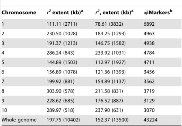
Table 2. Extent of linkage disequilibrium and number of
markers needed to reach average r2= 0.1 for individual
chromosomes and the whole genome.
Chromosome r2 extent (kb)a r2 sextent (kb) a #Markersb 1 111.11 (2711) 78.61 (3832) 6892 2 230.50 (1028) 183.25 (1293) 4963 3 191.37 (1213) 146.75 (1582) 4938 4 286.24 (843) 233.92 (1031) 4784 5 144.89 (1503) 112.97 (1927) 4711 6 156.89 (1078) 121.36 (1393) 3456 7 199.92 (881) 154.89 (1137) 3562 8 303.90 (578) 211.58 (831) 3719 9 228.62 (685) 176.52 (887) 3129 10 289.97 (518) 237.90 (631) 3070 Whole genome 197.75 (10402) 152.37 (13500) 43224 LD extent was computed with 43224 SNPs having MAF.0.05.
a
Physical distance to reach r2
or r2
sequal to 0.1 estimated using the non-linear
regression implemented in r-nls obtained by fitting Hill and Weir model [53]. r2
and r2
sobtained with Plink software [50] and r-LDcorSV [34], respectively. The
number reported in brackets indicates the number of equidistant markers that would be needed to reach an average r2of 0.1 between adjacent markers;
b
number of markers used to estimate LD extent for each chromosome and the whole genome.
Total diversity was higher in centromeric regions (Figure S17 in Text S1). Diversity within different genetic groups was slightly lower in centromeric regions (0.26 compared to 0.30 genome wide) and systematically for flints (0.21 for NF and 0.26 for EF) (Figure S17 in Text S1). This pattern was particularly clear on chromosomes 1, 2, 4, 6 and 8. Centromeric regions of these chromosomes also presented high relative differentiation among
groups (FST) (0.31, 0.21, 0.25 compared to 0.16 genome wide). For
other chromosomes, centromeres did not display a specific differentiation pattern.
Phenotypic variation for male (MFLW), female flowering time (FFLW), anthesis to silking interval (ASI) and association genetics
The analysis of the present design included eight additional field experiments compared to our previous studies which included only two experiments [21,30]. Plot heritability was 0.96, 0.97 and 0.45 for FFLW8, MFLW8 and ASI8, respectively. It confirmed high phenotypic variation for FFLW8 (sd = 168 GDD or 13.6 days), MFLW8 (sd = 161.5 GDD or 12.9 days), ASI8 (sd = 26 GDD or 2.2 days). This variation appeared to be closely related to the
population structure (R2= 0.51, 0.54 and 0.11 for FFLW8,
MFLW8 and ASI8, respectively). For FFLW8, the group adjusted means were 762 (641), 763 (635), 943 (673), 889 (623) and 1181 (633) for NF, EF, SS, CBD and Trop, respectively (see Table S5 in Text S1 for other traits).We tested several structure and kinship matrices for FFLW8 association studies in order to avoid an excess of false positives. Figure S18 in Text S1 illustrates the logarithm of
cumulative P-values obtained. The stronger correction was obtained with the model involving the kinship matrix calculated with 29911 Panzea SNPs. Adding a structure matrix did not change the P-values in that case. The models involving structure matrix calculated with 55 SSRs and either IBS or IBD kinship calculated with 94 SSRs were equivalent. Considering the limited differences between SSR and SNP based estimates of population
structure and kinship, we used the model Q55SSRs+KIBS(94SSRs)as
reference to avoid using SNPs as candidate loci and for population structure and kinship estimations. As illustrated by Figure S18 in
Text S1, P-values obtained with model Q55SSRs+KIBS(30KSNPs)
were globally higher than with Q55SSRs+KIBS(94SSRs). However,
most associations significant with P-values,1025 obtained with
model Q55SSRs+KIBS(94SSRs) remained highly significant
(P-val-ues,1023) with model Q55SSRs+KIBS(30KSNPs). P-values of the two
models were globally strongly related, the most notable exception being the centromeric region of chromosome 8, for which markers
with a P-value of 1027 Q55SSRs+KIBS(94SSRs) were never below
1023 with Q55SSRs+KIBS(30KSNPs). This probably relates to the
large number of markers in high LD in this region, which
consequently have an important contribution to the KIBS(30KSNPs)
kinship estimation (Rincent et al., pers. com.).
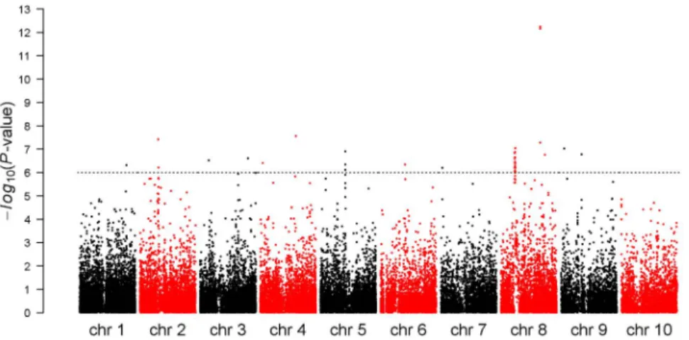
The association statistics obtained for FFLW8 are summarized
in Figure 2. The FDR 5% corresponded to P-value,1023.
Considering this threshold, 673 markers were associated with FFLW8, 843 with MFLW8 and 145 with ASI8. Among associations for FFLW8, 96 (corresponding to 18 regions) had a
P-value below 1025, 50 below 1026(corresponding to Bonferroni
correction) and 7 below 1027(corresponding to a break point in
Figure 1. Genome-wide linkage disequilibrium between all loci within and between chromosomes. The upper triangle corresponds to
the LD r2measure calculated with Plink [50], the lower triangle to the LD r2smeasure [34] corresponding to r
2
corrected for structure, using the Q matrix obtained with STRUCTURE software [40,41] and 55 SSRs. Values above 0.2 are highlighted by colored dots.
the P-value distribution, Figure S18 in Text S1). These two latter categories corresponded to 14 and 5 regions, respectively.
Considering MFLW8, 108 markers had P-values below 1025,
including 77 in common with FFLW8. For ASI8, seven markers
had P-values below 1025 and were not shared with FFLW8 or
MFLW8 (Table S6 and Table S7 in Text S1). When adding Vgt1 (presence-absence of the Mite allele), which has a strong effect on flowering time (7 days) according to [21], as a covariate in the model, all markers remained significant for FFLW8 (results not
shown). The estimated effects of markers having P-value,1025
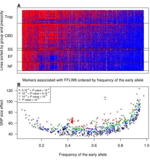
ranged from 44 (3.5 days) to 123.5 GDD (9.9 days), with a majority of small effects and a few strong effects (Figure S19 in Text S1). The bottom envelope in Figure 3 illustrates that loci with low MAF necessitate greater absolute effects to pass the significance threshold. We also observed that for the significant tests the early allele generally had the highest frequency and that the highest absolute effects corresponded to extreme frequencies (Figure 3). Estimated genetic variances associated with loci with significant effects ranged from 0 (after discarding a limited number of low negative values) to 34%, with three-quarters of the values below 10% (Figure S20 in Text S1) according to the linear mixed model (lmm) and from 0 to 9% according to the linear model (lm). The proportion of early alleles in one line was negatively correlated (20.84) with FFLW8 and therefore positively correlated with its precocity (Figure S21 in Text S1). This analysis was complemented by a multi-locus analysis of FFLW8 starting of the
96 markers with significant individual effects (P-value,1025). The
first marker included was ZCN8 (#23) as expected. The nine first
markers added in the model were significant with (P-value,1023)
conditionally to the previous model. The last marker entering the
model with (P-value,0.05) was the 29th. AIC then continued to
decrease until 71 markers were included in the model (see Table S8 for the order of inclusion of markers). The polygenic variance explained, once structure effect was removed, was 62% when considering the 29 first markers and 66% with 71 markers.
Finally, to avoid possible confusion between population structure and marker effects, we estimated marker effects with an ANOVA in three different genetic groups (flints, dents and
tropicals). For the 96 markers with P-value,1025for FFLW8 in
the entire panel and lmm, marker effects were higher in tropicals (median = 162 GDD) compared to dents (75 GDD) and flints (53 GDD). Among them, 70 were significant in tropicals, 34 in dents,
6 in flints (P-value,1023). All significant effects had the same sign
in the three genetic groups. In addition, 110 markers that were not significant in the entire panel were highly significant
(P-value,1026) in at least one group, 9 in flints, 63 in dents and
39 in tropicals, with a mean effect of 80, 120 and 230 GDD, respectively.
Regions with the highest contribution to flowering time variation
Table 3 summarizes information on the 18 most significant loci selected among cluster of loci along the genome and showing major contributions to flowering time variation according to
models Q55SSRs+KIBS(94SSRs)and Q55SSRs+KIBS(30KSNPs),as well as
10 additional loci strongly under selection. Regarding the first aspect, the marker that explained the highest genetic variance (24 and 9% for lmm and lm, respectively) with the highest P-value
(10213, 10212, 1024for FFLW8, MFLW8 and ASI8, respectively)
was located on chromosome 8 (#23 in Table 3, 123506141 bp),
5000 bp from the Zea CENTRORADIALIS gene ZCN8
(GRMZM2G179264, 123501085 bp). There was no other marker in the 50K Illumina array closer to this gene. Its effect was 108 GDD (9.7 days). It was 1 Mb apart from PZB02155.1 (124657056 bp), which was found to be associated with flowering time in the NAM population [4] but not in this panel when including structure in the model. It was 8 Mb apart from Vgt1 Mite (131984851 bp), a major flowering time QTL that has been
cloned [24]. Vgt1 Mite presented an association P-value,10214
with SAS GLM [32] and P-value,1029with lmm in this study.
LD (r2) between ZCN8 (marker #25) and Vgt1 Mite was 0.3. This
marker remained significant when adding Vgt1 Mite in the linear mixed model. ZCN8 was located between two flowering time meta QTL defined in the meta analysis of [22] (green meta QTL Vgt2 and blue meta QTL Vgt1 in Figure 3 of the above paper), between
marker pdc1 (118167604 bp) and marker umc1592
(125903155 bp), at the border of the Vgt1 QTL.
Other markers with a main contribution to FFLW8 were located on chromosomes 1 (#2), 2 (#5), 3 (#7,#9), 4 (#11), 5 (#14), 8 (#24), 9 (#27, #28), with a genetic variance ranging from 10 to 23% according to lmm and 3 to 6% according to lm. Ten additional loci displayed intermediary effects. According to the projection of flowering time meta QTL [10] on the maize sequence, seven associated markers were found in meta QTLs (#2, #4, #5, #6, #15, #16, #17). Five loci were next to one NAM [4] association (#9, #11, #15, #16, ZCN8 #23). Note that
Figure 2. Manhattan plot for female flowering (FFLW8) associations across the whole genome. P-values were obtained with the mixed model including the structure matrix obtained using STRUCTURE software and 55 SSRs and the kinship matrix obtained with 94 SSRs and IBS measure. Horizontal dashed line indicates Bonferroni-corrected 5% significance threshold.
some other markers with slightly lower P-values (1027
,P-value,1025) were close to NAM associations [4] and were
included in the meta QTLs [10] for the majority (#4, #6, #17, #21, #22). Several associated markers were close to ZCN genes and loci associated with flowering time in other studies (#4 5 Mb from ZCN4, 400 kb from NAM PHM3457.6, in meta QTL 2_4; #17, 200 kb from NAM PHM4748.16, 1 Mb from ZCN7, in meta QTL 6_3; #23 5000 bp from ZCN8, 1 Mb from NAM PZB02155.1; #16, in meta QTL 6_1, 1 Mb from ZCN15, 5 Mb from NAM PZA00355.2; #5: centromere of chromosome 2, 5 Mb from ZCN21, in meta QTL 2_4). Note that #15 may be involved in the sugar pathway as observed in Arabidopsis [68].
LD, diversity and differentiation at markers associated with FFLW8 and other regions under selection
Diversity and FST were higher at markers associated with
FFLW8 (P-value,1025) as compared to other parts of the genome
(HE of 0.42 compared to 0.36, FST of 0.27 compared to 0.16).
Within group diversity (HS) was also lower in these regions than for
the whole genome in NF (0.17) and EF (0.22) and in contrast higher in tropicals (0.4) (Figure S17 in Text S1, Figure S12). For these loci, the mean proportion of early alleles accumulated in NF, EF, SS, CBD and Trop non-admixed lines was 0.87, 0.83, 0.41, 0.48 and 0.39, respectively (Figure S22 in Text S1), consistent with the average flowering time of these groups. More balanced allele
frequencies in dent groups was noted in particular on centromere of chromosome 2 (#5), chromosome 3 (#9), 4 (#11) and 8 (#23 close to ZCN8, see above). ZCN8 (Vgt2 locus) appeared to be
strongly under diversifying selection (log10(PO) = 3.1). Allelic
frequencies at Vgt2 were slightly more differentiated than those observed for Vgt1 (for Vgt1 and Vgt2, the early allele was fixed in NF, frequencies were 0.94 and 0.97 in EF, 0.5 and 0.7 in CBD, 0.17 and 0.13 in tropicals, respectively). As shown in Figure S11, the region between Vgt2 and Vgt1 was characterized by low diversity in flints and a low recombination rate. Differentiation was high only around Vgt2.
Besides these diversity trends, regions associated with flowering
time also displayed higher LD (r2= 0.2 compared to 0.14 for the
entire genome) and lower recombination (0.02 compared to 0.04). The major haplotype in these regions was shared by 65% of lines (compared to 50% for the whole genome) (Figure S11).
In addition, some markers were found to be under selection although not related to flowering time in this panel. They nevertheless were related to flowering time according to other studies (#1, in meta QTL 1_5, 4 Mb from an association with
P-value 1025; #3 1 Mb from Phyc1; #18, 200 kb from NAM
PZA02722.1. This suggests that the association mapping power at these loci may have been hindered by fixation in some of the groups.
Figure 3. Distribution of SNP effects (GDD) according to the early allele frequency. In this figure, 673 markers with P-value,1023are
represented. (A) For all inbred lines (rows) and SNPs (columns), red and blue colors correspond to the presence of late and early alleles, respectively. (B) The absolute SNP effect versus the frequency of the early allele for significant associations. Different colors correspond to different P-value thresholds.
Table 3. Regions associated with FFLW8 (P -value below 10 2 5) ) and/or under selection (log 10 (PO ) above 0.5). Nb Marker Name a Cent b Chr c Pos d P -value e Effect f P -value nc g R 2lm h R 2lmm i PO j FST k Meta QTL l Gene ID m Gene Descr n Gene Dist (bp) o 1 PZE-101106079 0 1 109 3 94 965 1.39E-01 2 19.41 1.00E-16 0 .02 0.07 0.77 0.51 1 _5 GRMZM2G041613 uncharacterized 0 2 S YN13483 0 1 2 49 324 652 6.64E-06 2 82.29 1.05E-05 0 .03 0.11 2 1.69 0.00 1 _10 GRMZM2G103843 ribokinase a ctivity 0 3 S YN19258 0 1 2 78 034 859 7.75E-01 2 3.98 4.56E-02 0 .00 0.02 1.49 0.59 -GRMZM2G328224 transferase activity on hexosyl groups 0 4 PZE-102079486 0 2 62 516 828 3.43E-06 2 70.49 4.42E-12 0 .04 0.08 2 2.09 0.13 2 _4 GRMZM2G084462 tRNA isopentenyltransferas e activity 0 5 PZE-102086452 1 2 78 699 684 3.87E-08 7 6.55 1.00E-16 0 .06 0.23 2 1.62 0.34 2 _4 GRMZM2G474153 p rotein kinase activity 0 6 S YN12061 0 2 1 99 457 622 7.10E-06 5 1.01 5.64E-07 0 .04 0.09 2 1.45 0.00 2 _5 GRMZM2G400173 transporter a ctivity 0 7 PZE-103099066 0 3 159 5 26 813 1.E-06 62.64 1.E-16 0 .06 0.14 2 2.22 0.16 -GRMZM5G891247 enzyme inhibitor a ctivity 47 249 8 PZE-103098863 0 3 159 1 70 263 6.48E-01 2 7.92 7.53E-14 0 .00 0.06 1.41 0.68 -GRMZM2G082608 uncharacterized 0 9 PZE-103145047 0 3 199 9 53 486 2.49E-07 2 61.64 1.00E-16 0 .04 0.13 2 2.08 0.37 -GRMZM5G886883 uncharacterized 0 10 PZE-104010434 0 4 7 5 67 350 3 .03E-01 1 4.95 3.56E-02 0 .00 0.00 1.05 0.55 -GRMZM2G012821 uncharacterized 49 496 11 PZE-104013311 0 4 11 576 332 3.94E-07 6 5.35 7.35E-05 0 .05 0.17 2 2.02 0.22 -GRMZM2G113241 uncharacterized 50 532 12 PZE-104080388 0 4 154 6 89 801 2.77E-08 2 85.74 3.33E-16 0 .03 0.00 2 1.92 0.20 -GRMZM2G138407 transcription factor activity 106 768 13 PZE-105049333 0 5 40 625 928 3.77E-01 1 2.11 5.02E-01 0 .01 0.02 1.14 0.58 5 _4 GRMZM2G150893 peroxidase activity 119 669 14 PZE-105082545 0 5 97 872 011 1.28E-07 2 66.39 5.43E-12 0 .04 0.10 2 1.75 0.50 -GRMZM2G018962 e xostosin-like protein 351 398 15 PZE-105130917 0 5 187 8 48 427 4.93E-06 2 63.67 4.10E-13 0 .03 0.07 2 2.18 0.15 5 _6 GRMZM2G159918 transferase activity on hexosyl groups 0 16 PZE-106032161 0 6 74 959 244 2.01E-06 5 9.17 1.11E-16 0 .03 0.08 2 2.15 0.34 6 _1 GRMZM2G005499 transmembrane transport 0 17 SYN38078 0 6 1 58 225 752 4.43E-06 2 61.61 5.16E-06 0 .03 0.02 2 2.00 0.17 6 _3 GRMZM2G074792 intracellular zinc ion binding 0 18 SYN18613 0 7 1 50 876 445 5.64E-01 8.61 9.32E-01 0 .00 0.00 3.10 0.67 -GRMZM2G038449 uncharacterized 11 523 19 PZE-108038931 1 8 45 270 084 9.38E-08 2 69.31 8.99E-15 0 .03 0.03 2 1.81 0.37 -GRMZM2G142870 A TPase a ctivity 0 20 PZE-108035509 1 8 52 084 948 3.05E-02 3 5.04 9.56E-09 0 .01 0.12 2.85 0.61 -GRMZM2G006585 zinc ion binding 5783 21 PZE-108053909 0 8 95 953 461 5.50E-01 8.45 6.87E-02 0 .01 0.03 1.32 0.58 8 _3 GRMZM2G074645 transcription factor activity 174 238 22 SYN12978 0 8 1 20 970 129 6.93E-01 5.07 1.00E-16 0 .01 0.00 0.63 0.36 -GRMZM2G473111 uncharacterized 0 23 PZE-108070380 0 8 123 5 06 141 5.88E-13 1 07.83 1.00E-16 0 .09 0.24 3.10 0.71 -GRMZM2G179264 ZCN8 protein 5056 24 PZE-108081330 0 8 138 2 62 446 2.E-07 81.15 1.E-16 0 .06 0.34 2 1.58 0.34 -GRMZM2G164341 transcription factor activity 0 25 PZE-108089589 0 8 146 5 55 253 2.32E-01 2 18.36 1.11E-03 0 .00 0.00 1.02 0.58 -GRMZM2G094165 carbonate d ehydratase activity, binding 0 26 PZE-109008014 0 9 8 9 44 436 9 .45E-08 6 7.29 7.12E-12 0 .03 0.02 2 2.07 0.20 -GRMZM2G142072 transcription e longation regulator activity 0
Discussion
Suitability of the 50K Illumina array for investigating line similarities, panel structures and local diversity trends along the genome
Ascertainment bias due to the marker type and selection can be a concern in diversity analyses. We confirmed that considering an overrepresented set of B73 (SS)6Mo17 (CBD) SNPs lead to overestimated genetic distances for dent (CBD and SS) lines (Figure S5 in Text S1), as observed in other studies [31,69]. When excluding these markers and considering only Panzea SNPs, we did not observe this trend and obtained population structure results that were highly consistent with those obtained with 55 SSRs, including mostly trinucleotides and more (Figure S8 in Text S1). The differentiation between groups was also consistent between SNPs and SSRs, with the greatest differentiation noted between NF and SS (Table S2 in Text S1). This illustrates that when based on a relevant marker sample, although not leading to the discovery of new polymorphisms as compared to other approaches like GBS [70] or sequencing [71], SNP arrays can be a powerful tool for investigating population structure.
The average genetic diversity of the panel calculated with Panzea SNPs was 0.36. This value was in the upper range of those reported by other diversity analyses based on SNP genotyping, ranging from 0.27 to 0.39 [72,73,74,75,76]. Only eight percent of markers appeared to be monomorphic, showing that some rare alleles discovered with the Panzea panel used to build the 50K Illumina array were not represented in our panel. Considering the MAF distribution, we observed a lower proportion of rare alleles (,0.1) compared to other frequency classes and a slight excess of intermediate alleles (Figure S3 in Text S1). This frequency profile clearly deviates from the L-shaped pattern (excess of rare alleles) expected at mutation drift equilibrium in the absence of bias in polymorphism discovery [77]. This could be the result of specific evolutionary processes and/or the experimental strategies used during marker assembly. The deficit in rare alleles may be due to some extent to SNP discovery, which was mostly based on 27 lines [36,78] and followed by quality and polymorphism criteria in favor of balanced polymorphisms [31]. The slight excess in intermediate frequency alleles was consistent with the high enrichment in intermediate frequency alleles observed for three genomic regions that were sequenced (Figure S3 in Text S1). This could be related to allelic differentiation between groups due to drift and diversifying selection for some regions.
Beyond these trends for the global panel, we also noticed contrasted frequency patterns across genetic groups. The high deficit in rare alleles in tropicals was probably due to their under-representation (relative to their very high diversity) at the SNP discovery step. Other groups passed comparable sampling procedures, so the differences that were observed suggest the involvement of different evolutionary processes.
Fifteen percent of loci were monomorphic in flints, compared to 2% only in CBD and tropicals (Table 1). When looking at alleles that were rare in tropicals (,0.05), the difference was even more striking, with 30% of alleles lost in flints compared to only 6% in dents. In contrast, some alleles that were originally rare in tropicals reached near fixation in flints (NF and EF) (Figure S4 in Text S1). This suggests that the NF group passed severe bottleneck(s) when diverging from tropical germplasm approx. 1900 years ago [79,80]. The relative (compared to other groups) overabundance of rare alleles observed for Northern Flints suggests that the population expansion that followed the differentiation of this group was accompanied by limited introgression by external genetic groups. Table 3. Cont. Nb Marker Name a Cent b Chr c Pos d P -value e Effect f P -value nc g R 2lm h R 2lmm i PO j FST k Meta QTL l Gene ID m Gene Descr n Gene Dist (bp) o 27 PZD00049.4 0 9 1 7 0 19 800 2.E-06 72.63 1.E-16 0 .04 0.10 2 1.70 0.32 -AC197699.3 transcription factor activity 0 28 PZE-109038470 0 9 57 186 011 1.70E-07 9 4.50 1E-16 0 .04 0.17 2 2.10 0.19 -GRMZM2G076272 transcription factor activity 0 aIllumina marker name; bif marker in centromeric region according to m aize GDB and. [66] flanking m arkers, then 1, else 0; cphysical chromosome; dphysical position in R efGen_v2; emarker P -value for female flowering in g rowing degree days base temperature 8 (FFLW8) according to model Q55SSRs + KIBS(94SSRs) ; fmarker effect on FFLW8 according to model Q55SSRs + KIBS(94SSRs) ; gmarker P -value for FFLW8 according to n aı¨ ve model; hpercentage o f variance explained by the m arker in a linear model Q55SSRs ; ipercentage o f variance explained by the m arker in a linear m ixed model Q55SSRs + KIBS(94SSRs ) ; jlog 10 (posterior odds) for selection test obtained with BayeScan [47], significant (highly) when . 0( . 1); kdifferentiation index calculated w ith r-Hierfstat [46] using non-admixed lines; lmeta QTL n ame (adapted from [10]): meta QTL X _Y with X the chromosome number e t Y the Q TL number; mname o f closest annotated gene according to R efGen_v2; nclosest annotated gene function; odistance between marker a nd closest annotated gene. doi:10.1371/journal.pone. 0071377.t003
As stated above, the level of polymorphism observed in CBD presented only limited loss compared to tropical materials. Alleles that were observed in flints while being rare or absent in tropicals were also generally noted in dents (CBD), whereas the reverse was not true. This is consistent with CBD originating in part from flints (NF) and in part from a group relatively close to tropicals, approx. 400 ago [81]. The relative deficiency in rare alleles observed for CBD (Figure S3 in Text S1) confirmed that they emerged recently from a restricted number of founders from these two origins [82]. When comparing European flint diversity to that of Northern flints, we found that 93% of alleles were common to both groups, which was higher than in previous studies with multiallelic markers (75%) [83,84]. Some alleles (5410) observed in EF were absent in NF. These alleles were generally also observed in non-admixed CBD (89%) or tropicals (94%). This confirms that EF is a recent group mainly derived from NF after their introduction into Europe and subsequent hybridization with materials of tropical origin, probably different from those used to form CBD [84]. Consistent with these trends, we observed a lower genetic diversity for NF (0.28) and EF (0.30) relative to CBD (0.35) and tropicals (0.34).
Linkage disequilibrium and estimation of marker density required for association studies
The genotyping method we used did not allow us to estimate LD at the gene level as obtained by [85] but was adequate to reveal the LD structure at the genome level when considering a wide diversity of lines (tropicals, Corn Belt Dents, Northern and European Flints).
LD between unlinked or distant polymorphisms was globally
low in the panel (quantile 95% of 1025 between different
chromosomes) with, however, notable exceptions between centro-meric regions of chromosomes 1, 5, 8 and a few additional regions, like the extremity of chromosome 10 (Figure 1). Correction for the
population structure (r2s) clearly removed long distance LD
(Figure 1, Figure S15 in Text S1), especially LD among centromeres of different chromosomes. Some pairs of markers
located on different chromosomes still presented r2s above 0.2.
This could suggest that we did not perfectly correct the measure for the structure effect and that alternative approaches such as
calculating r2vs [34] that corrects for relatedness should be
considered. Alternatively, LD between unlinked loci may be due to loci that are involved in common functions and subjected to joint selection pressure.
For closely linked polymorphisms, we observed a rapid decrease
in r2values as the physical distance between SNPs increased. The
fitted LD values obtained with the non-linear model [53] and the average obtained by the distance class approach were close. This suggests that the Hill and Weir model [53], taking into account the sample size and mutation rate, was more realistic than the Sved model [52] which hypothesised that the size of the panel was equal to the effective population size, the panel had undergone no selection or mutations and the recombination rate was constant along the genome. According to the Hill and Weir model, LD dropped below 0.1 after 200 kb at the genome level and dropped to almost the background level at around 500 kb-1 Mb. This value was in the range of those reported in the literature for different types of panels [85,86,87,88] and illustrates that linkage disequi-librium in maize has markedly increased as a result of domestication [1] and genetic improvement [2,74,89]. We observed that the extent of LD varied among chromosomes, i.e. 100 kb on average along chromosome 1, between 140 and 200 kb on average along chromosomes 5, 6, 3 and 7, between 200 and 300 kb along chromosomes 9, 2, 4, 10 and 8, which suggests
different selection pressures were involved. Note that this ranking apparently varies among populations [74,89]. Extracting the variation due to population structure did not much change these trends, with an average decrease of around 150 kb instead of
198 kb. We noticed that correction of r2by the r2sestimator was
generally less marked than for Vitis vinifera [34]. This suggests that the maize genetic groups considered in our study were less differentiated than groups of grape varieties corresponding to different uses (table vs. wine production).
Visualization of LD as a sliding window (1 Mb) approach revealed high variation along chromosomes (Figure S11). It confirmed a general trend of higher LD in centromeres, as expected given the low recombination rate of these regions [31,36]. This was especially noteworthy on chromosomes 7, 8 and 10. We noted that, according to LD and the diversity profiles, the position of the centromere of chromosome 5 obtained by [66] was probably more realistic than that recorded in MaizeGDB (maizegdb.org) (Figure S11, S12). With the FastPHASE algorithm, we observed one predominant ancestral haplotype shared by 67% of lines in centromeric regions, in contrast to the rest of the genome, which presented more balanced frequencies of ancestral haplotypes, with the predominant one being shared by 53% of lines. The probability of haplotype switch from one SNP to another computed with FastPHASE was also lower in these regions. Interpreting these probabilities as recombination rates could be questioned [55], but, overall, these results are consistent with the hypothesis that centromeres have undergone less recombination since domestication as compared to the rest of the genome. This could be due to mechanical obstacles to recombination and gene flow in the vicinity of centromeres and/or selection forces that preferentially occur in these regions [78,90,91,92]. High differentiation rates, indicating selection forces, were indeed observed for centromeres of chromosomes 3,
5, 6 and 8 (FSTof 0.22, 0.21, 0.25, 0.31, respectively, compared to
0.16 on average on the genome). Differentiation at some centromeric regions was also observed by [1] in a panel that included wild relatives.
We detected peaks of LD outside centromeres that suggested different local histories of recombination [78] and highlighted some putative selective events involved in flowering time or other adaptive traits. The highest local LD was observed between Su1 [93,94,95,96], Tga1 [97] and Bt2 on chromosome 4, a region involved in carbohydrate metabolism [98,99] known to have
played a key role in maize domestication. Generally, a r2of 0.10 is
considered to be the minimum LD value needed to detect associations with complex traits. This reasoning is based on a large
effect QTL that explains 10% of phenotypic variation (h2q= 0.1),
which is a rather high expectation according to present knowledge, as also discussed by Van Inghelandt et al. [89]. Detection of markers that explain 10% of polymorphism at such QTLs
(r2= 0.1) and thus 1% (r2|h2q) of the phenotypic variation could
be considered as a minimum to have acceptable power with panel sizes classically used in plants (generally several hundred individ-uals) [100]. QTLs which explain less than 10% of the phenotypic variation would then require higher LD and/or higher panel size to achieve the same power [101]. Given LD decrease values obtained in this study and considering that the size of the maize
genome is around 2.5 109bp [102], an average r2of 0.1 or 0.3
between adjacent markers would be expected when using 10450 (Table 2) or 75000 markers evenly distributed across the genome.
The 50K Illumina array should be sufficient to obtain a global r2s,
which better reflects the power of association genetics considering the population structure [34], of 0.1 but not 0.3. We would therefore require 100000 markers with higher density on