HAL Id: hal-01646782
https://hal.archives-ouvertes.fr/hal-01646782
Submitted on 23 Nov 2017
HAL is a multi-disciplinary open access
archive for the deposit and dissemination of
sci-entific research documents, whether they are
pub-lished or not. The documents may come from
teaching and research institutions in France or
abroad, or from public or private research centers.
L’archive ouverte pluridisciplinaire HAL, est
destinée au dépôt et à la diffusion de documents
scientifiques de niveau recherche, publiés ou non,
émanant des établissements d’enseignement et de
recherche français ou étrangers, des laboratoires
publics ou privés.
Constructive Type Theory of Coq
Christian Doczkal, Joachim Bard
To cite this version:
Christian Doczkal, Joachim Bard. Completeness and Decidability of Converse PDL in the Constructive
Type Theory of Coq. Certified Programs and Proofs, Jan 2018, Los Angeles, United States.
�hal-01646782�
Completeness and Decidability of Converse PDL in
the Constructive Type Theory of Coq
Christian Doczkal
∗Univ Lyon, CNRS, ENS de Lyon, UCB Lyon 1, LIP christian.doczkal@ens-lyon.fr
Joachim Bard
Saarland University
Abstract
The completeness proofs for Propositional Dynamic Logic (PDL) in the literature are non-constructive and usually pre-sented in an informal manner. We obtain a formal and con-structive completeness proof for Converse PDL by recasting a completeness proof by Kozen and Parikh into our con-structive setting. We base our proof on a Pratt-style decision method for satisfiability constructing finite models for sat-isfiable formulas and pruning refutations for unsatsat-isfiable formulas. Completeness of Segerberg’s axiomatization of PDL is then obtained by translating pruning refutations to derivations in the Hilbert system. We first treat PDL without converse and then extend the proofs to Converse PDL. All results are formalized in Coq/Ssreflect.
1
Introduction
Propositional Dynamic Logic (PDL) [12, 15] is a modal logic developed for reasoning about programs with applications for instance in knowledge representation [3]. The modalities of PDL are given by regular programs (i.e., regular expres-sions with tests) describing binary relations on states. The formula [α ]φ is satisfied by some state if all α -reachable states satisfy φ. The language of programs includes a re-flexive transitive closure operation (α∗) causing PDL to be non-compact. Converse PDL (CPDL), also defined in [12], extends PDL with a converse operation on programs. Both PDL and CPDL have the small-model property [12] and are EXPTIME-complete [12, 21]. Axiomatizations of PDL and CPDL were first given by Segerberg [22] and shown complete independently by Gabbay [13] and Parikh [19].
Our main result is a machine-checked constructive proof that for every PDL or CPDL formula φ one can either con-struct a proof of ¬φ from the respective axioms or a model of
∗This author has been funded by the European Research Council (ERC)
under the European Union’s Horizon 2020 programme (CoVeCe, grant agreement No 678157).
This work was supported by the LABEX MILYON (ANR-10-LABX-0070) of Université de Lyon, within the program “Investissements d’Avenir” (ANR-11-IDEX-0007) operated by the French National Research Agency (ANR). CPP 2018, January 8 – 9, 2018, Los Angeles, CA, USA
This is the author’s version of the work. It is posted here for your personal use. Not for redistribution. The definitive Version of Record will appear in Proceedings of the 7th International Conference on Certified Programs and Proofs, January 8 – 9, 2018.
bounded size satisfying the formula. Completeness and the small-model property as well as decidability of satisfiability, validity and provability then follow as corollaries. The form of constructive completeness result established here is more informative than a classical completeness result in the sense that it provides an algorithm constructing proofs for valid formulas rather than merely showing the existence of such proofs.
The completeness proofs for (C)PDL in the literature either use non-standard canonical models and filtration [15, 19] or construct “canonical” models inside a finite syntactic uni-verse [18]. Both techniques are non-constructive in the sense that they assume (at least) logical decidability of provability (i.e., ⊢ φ ∨ ̸⊢ φ for all φ). While logical decidability follows from (computational) decidability, the easiest way to show decidability of provability is via completeness.
In order to obtain a constructive completeness result, we base the completeness proof on a decision method for satis-fiability. We employ a variant of pruning [17, 21] extended to provide refutations for unsatisfiable formulas in addition to constructing models for satisfiable formulas. Translating these pruning refutations to proofs in the Hilbert system then yields the desired completeness result. The use of prun-ing as decision procedure underlyprun-ing the completeness result naturally leads to a factorization of the proof into an algo-rithmic part for the decision method, a semantic argument for the model construction, and a syntactic translation from pruning refutations to Hilbert refutations. We believe that the constructive nature of the proof and the clear separation of concerns makes the proof particularly easy to follow.
The pruning-based approach is inspired by completeness proofs for the branching time logics UB (“unified branch-ing”) [5] and Computation Tree Logic (CTL) [11] and was employed by the first author to obtain formal and construc-tive completeness proofs of Hilbert and sequent systems for CTL [8, 10]. For the construction of models using pruning, we follow the presentation of pruning in [16]. The transla-tion from pruning refutatransla-tions to Hilbert proofs builds on ideas in [18]. For CPDL, we show that the Hilbert system val-idates the conversion of formulas to converse normal form and then use pruning for converse normal formulas. This isolates the treatment of converse to a few select places in the proof. We are not aware of any other completeness proof treating converse this way.
The mathematical proofs described in this paper are con-structive and designed with the formalization in mind. The accompanying Coq development [9] follows the proofs out-lined in the paper and provides the details elided in the paper. The development is carried out using the Ssreflect [14] proof language and the Mathematical Component Libraries [25]. Our development builds upon the formal and constructive completeness proof for test-free PDL presented in [4].
The rest of the paper is organized as follows. Section 2 recalls the syntax, semantics, and Hilbert system of PDL and describes their representation in Coq. Sections 3 to 6 describe the constructive completeness result for PDL. Sec-tion 7 describes the changes required to extend our results to CPDL. Section 8 provides a high-level overview of the accompanying Coq development [9].
2
Propositional Dynamic Logic
We fix a countably infinite type of atomic programs A and a countably infinite type of atomic propositions P. The letter a ranges over atomic programs and the letter p ranges over atomic propositions. We consider Propositional Dynamic Logic (PDL) with the following syntax for programs (denoted α, β, . . . ) and formulas (denoted φ,ψ , . . .).
α, β B a | α + β | α β | α∗| φ? (a : A) φ,ψ B p | ⊥ | φ → ψ | [α]φ (p : P) We define the remaining logical operations in terms of this syntax (i.e., ¬φ B φ → ⊥, φ ∧ ψ B ¬(φ → ¬ψ ), ⟨α⟩φ B ¬[α ]¬φ, . . . ).1We write |φ| and |α | for the sizes of formulas and programs (i.e., the size of the syntax tree).
Formulas are interpreted over transition systems where the states are labeled with atomic propositions and the tran-sitions are labeled with atomic programs. A transition sys-tem M hence consists of
• A (possibly infinite) type |M | whose elements are called states
• A transition relation⇒aM : |M | → |M | → Prop for
every a : A
• A labeling LM : P → |M | → Prop.
In the following, we write M for transitions systems as well as their underlying type of states.
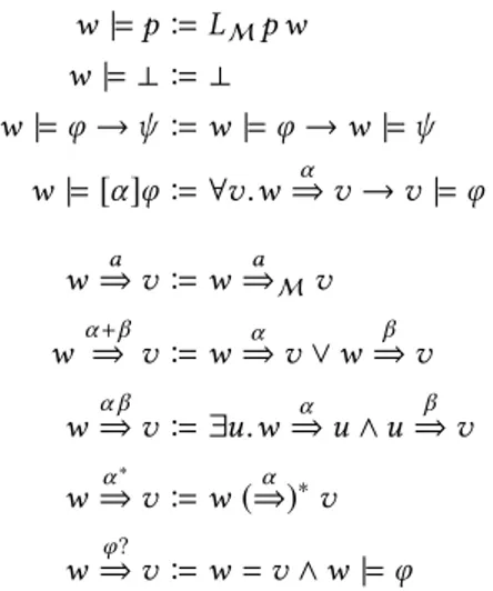
Let M be a transition system. We define a satisfaction relation between states w of M and formulas φ, written w |= φ, and an interpretation of programs α as binary rela-tions on M, written⇒ (with M implicit), by mutual recur-α sion on formulas and programs (cf. fig. 1). Note that we use the same symbols (e.g. →) both for the logical operators of PDL and for those of the type theory. This does not lead to ambiguity.
1Whileφ → ψ could be defined as [φ?]ψ , we include it in the syntax since
this allows us to define the Hilbert system with minimal reliance on defined logical operations. w |= p B LMp w w |= ⊥ B ⊥ w |= φ → ψ B w |= φ → w |= ψ w |= [α]φ B ∀v.w⇒ v → v |α = φ w ⇒ v B wa ⇒aMv w α +β⇒ v B w⇒ v ∨ wα ⇒ vβ w α β⇒ v B ∃u.w⇒ u ∧ uα ⇒ vβ w α ∗ ⇒ v B w (⇒)α ∗v w ⇒ v B w = v ∧ w |= φφ?
Figure 1. Semantics of formulas and programs
Our goal is to show soundness and completeness of the Hilbert system for PDL presented in fig. 2. The Hilbert sys-tem employed here is a variant of Segerberg’s axiomatization as presented in [15]. We replace the original induction axiom (i.e., [α∗](φ → [α ]φ) → φ → [α∗]φ) with a rule (Ind) and omit ⊢ φ → [α ][α∗]φ → [α∗]φ, which is derivable by
induc-tion. We prefer the system from fig. 2 because, a priori, it appears weaker. Nevertheless, it is straightforward to show that the two systems are equivalent (see [9] for the details). Hence, all our results apply to both systems.
The satisfaction relation essentially constitutes a shallow2
embedding of the classical object logic PDL into the construc-tive type theory of Coq. In order to ensure that the object logic is interpreted classically we restrict our attention to those transition systems for which the satisfaction relation is stable under double negation.
Definition 2.1. A (classical) model is a transition system M for which |= is stable under double negation, i.e., a transition system satisfying
∀w : M ∀φ.¬¬(w |= φ) → w |= φ (*) Classical models can be understood in several ways. The condition (*) localizes the classical assumptions required for soundness into the definition of models. In fact, classical models are the largest class of models for which one can constructively show soundness of the Hilbert system for PDL given in fig. 2.
Theorem 2.2 (Soundness). Let M be a transition system. Then ⊢ is sound for M (i.e., ⊢ φ implies w |= φ for all φ and all w : M) if and only if M is a classical model.
2Here, shallow refers to the fact thatw |= φ is just a proposition talking
about some relations over an arbitrary type. 2
Completeness and Decidability of Converse PDL in Coq CPP 2018, January 8 – 9, 2018, Los Angeles, CA, USA ⊢ φ → ψ → φ (1) ⊢ (θ → φ → ψ ) → (θ → φ) → θ → ψ (2) ⊢ ¬¬φ → φ (3) ⊢ [α ](φ → ψ ) → [α ]φ → [α ]t (4) ⊢ [α ]φ → [β]φ → [α+ β]φ (5) ⊢ [α+ β]φ → [α]φ (6) ⊢ [α+ β]φ → [β]φ (7) ⊢ [α β]φ → [α ][β]φ (8) ⊢ [α ][β]φ → [α β]φ (9) ⊢ [α∗]φ → φ (10) ⊢ [α∗]φ → [α ][α∗]φ (11) ⊢ [φ?]ψ ↔ (φ → ψ ) (12) MP ⊢ φ → ψ ⊢ φ ⊢ ψ Nec ⊢ φ ⊢ [α ]φ Ind ⊢ φ → [α ]φ ⊢ φ → [α∗]φ Figure 2. Hilbert system for PDL
Note that every transition system is a classical model if one assumes excluded middle. Moreover, one can show con-structively that all finite transition systems (with boolean transition relations and labeling) are classical models. This amounts to proving decidability of the model-checking prob-lem – which in the case of PDL is straightforward. Since PDL has the small-model property, we only need to construct finite models to show completeness.
For the rest of the paper, the word model always means classical model. We say that a formula φ is satisfiable if w |= φ for some state w of some model and valid if w |= φ for every state w of every model.
The main result of this paper is a constructive proof that for every formula φ, one can either construct a finite model certifying the satisfiability of φ or a proof of ¬φ from the axioms in fig. 2 (certifying the unsatisfiability of φ). Com-pleteness of the Hilbert system (i.e., ⊢ φ whenever φ is valid) as well as decidability of satisfiability, validity and provability then follow as corollaries.
The central notions in the completeness proof are the notions of demo, subformula universe, and pruning. Demos are a class of finite syntactic models designed such that for every subformula universe U , there exists a largest demo over U satisfying all satisfiable formulas in U . We construct this largest demo using pruning in such a way that we obtain proofs of ¬φ for all unsatisfiable formulas φ in U .
3
Subformula Universes
We now define the notion of subformula universe. A sub-formula universe for a sub-formula φ is a finite set of signed
formulas [23] containing all formulas that play a role in deciding satisfiability of φ.
Definition 3.1. We call a finite set F of formulas subformula closed if it satisfies the following closure properties:
S1. If φ → ψ ∈ F , then {φ,ψ } ⊆ F . S2. If [a]φ ∈ F , then φ ∈ F . S3. If [α+ β]φ ∈ F, then {[α]φ, [β]φ, φ} ⊆ F. S4. If [α β]φ ∈ F , then {[α ][β]φ, [β]φ, φ} ⊆ F . S5. If [α∗]φ ∈ F , then {[α ][α∗]φ, φ} ⊆ F . S6. If [ψ ?]φ ∈ F , then {ψ , φ} ⊆ F .
Note that subformula closedness requires the presence of more than just the subformulas of every formula (e.g., [α ][α∗]φ when [α∗]φ ∈ F ).
It is a standard result about PDL that every formula is included in a subformula closed set of size linear in |φ| called the Fisher-Ladner closure [12, 15] of φ. This closure be com-puted using two mutually recursive functions FL and FL□as
follows: FL(p) B {p} FL(⊥) B {⊥} FL(φ → ψ ) B {φ → ψ } ∪ FL(φ) ∪ FL(ψ ) FL([α ]φ) B FL□(α, φ) ∪ FL(φ) FL□(p, φ) B {[p]φ} FL□(α+ β, φ) B {[α + β]φ} ∪ FL□(α, φ) ∪ FL□(β, φ) FL□(α β, φ) B {[α β]φ} ∪ FL□(α, [β]φ) ∪ FL□(β, φ) FL□(α ∗, φ) B {[α∗ ]φ} ∪ FL□(α, [α ∗ ]φ) FL□(ψ ?, φ) B {[ψ ?]φ} ∪ FL(ψ )
In order to show that FL(φ) is subformula closed, we first es-tablish the following transitivity property. The proof follows the presentation in [15].
Lemma 3.2. 1. φ ∈FL(φ) and [α ]φ ∈ FL□(α, φ).
2. If ψ ∈FL(φ), then FL(ψ ) ⊆ FL(φ).
3. If ψ ∈FL□(α, φ), then FL(ψ ) ⊆ FL□(α, φ) ∪ FL(φ).
Proof. Claim (1) is trivial. Claims (2) and (3) follow by mutual induction on φ for (2) and α for (3). □ Lemma 3.3. FL(φ) is subformula closed.
Proof. Immediate with lemma 3.2(1) and lemma 3.2(2). □ Lemma 3.4. |FL(φ)| ≤ |φ| and |FL□(α,ψ )| ≤ |α |.
Proof. By mutual induction on φ and α . □ For the definition of subformula universes, we employ signed formulas. A signed formula has the form φσ where φ is a formula and σ ∈ {−,+} is its sign. Signs never occur within a formula and bind weaker than formula constructors, e.g, [α ]φ+ is to be read as ([α ]φ)+. Semantically, negative signs correspond to top-level negations. That is, w |= φ−is
to be read as w ̸|= φ and w |= φ+as w |= φ. In particular, we have:
w |= [α]φ−
⇔ ∃v.w⇒ v ∧ w |α = φ− ⇔ w |= ⟨α⟩¬φ Definition 3.5 (Subformula Universe). Let F be a subfor-mula closed set. We refer to the set { φσ | φ ∈ F , σ ∈ {+, −} } as the subformula universe over F . For formulas φ, we write U (φ) for the subformula universe overFL(φ).
Signed formulas are a technical device allowing us to de-scribe demos and pruning, which are usually dede-scribed using negation-normal formulas, in terms of our minimal syntax for PDL.
4
Demos
A clause is a finite set of signed formulas. Demos [16, 17] are certain sets of clauses that can be seen as models in such a way that every state satisfies all signed formulas it contains. The first requirement on demos is that all states are Hin-tikka sets.
Definition 4.1. A clause H is called a Hintikka set if satisfies the following closure conditions.
H1. ⊥+< H .
H2. There is no formula φ such that {φ+, φ−} ⊆ H . H3. If (φ → ψ )+∈ H , then φ−∈ H or ψ+∈ H . H4. If (φ → ψ )−∈ H , then φ+∈ H and ψ−∈ H . H5. If [α β]φσ ∈ H , then [α ][β]φσ ∈ H . H6. If [α + β]φ+∈ H , then [α ]φ+∈ H and [β]φ+∈ H . H7. If [α + β]φ−∈ H , then [α ]φ−∈ H or [β]φ−∈ H H8. If [α∗]φ+∈ H , then φ+∈ H and [α ][α∗]φ+∈ H . H9. If [α∗]φ−∈ H , then φ−∈ H or [α ][α∗]φ−∈ H . H10. If [φ?]ψ+∈ H , then φ−∈ H or ψ+∈ H . H11. If [φ?]ψ−∈ H , then φ+∈ H and ψ−∈ H .
Intuitively, Hintikka sets are clauses that are consistent with respect to state-local reasoning. Note that if φσ ∈ U for some subformula universe U , then all formulas mentioned in the Hintikka condition for φσ are also in U . The use of signs avoids the need to close subformula universes under adding/removing top-level negations (as is, for instance, done in [11]) thus simplifying the reasoning about the closure properties of the subformula universes.
Every finite set of clauses S, can be seen as a model M(S) in the following way:
|M(S)| B S
H ⇒a M(S)H′B { φ | [a]φ ∈ H } ⊆ H′ LM(S)p H B p+ ∈ H
Even for sets of Hintikka sets, the states of M(S) will generally not satisfy all the formulas they contain. To see this, recall that [a]p−corresponds to the diamond formula ⟨a⟩¬p, and consider the case where S B {{[a]p−, p+}}. Then the only state of M(S) lacks the a-successor satisfying p− required by [a]p−.
Definition 4.2. Let S be a finite set of clauses. We interpret programs as relations on S in the following way:
C⇝aSD B { φ+ | [a]φ+∈ C } ⊆ D Cα +β⇝SD B C⇝αSD ∨ C⇝βSD Cα β⇝SD B ∃E ∈ S.C⇝αSE ∧ E⇝βSD Cα ∗ ⇝SD B C (⇝αS)∗D C⇝φ?SD B C = D ∧ φ ∈ C
Remark 1. The set library employed in the formalization only allows us to write down sets that are finite by construc-tion. However, finiteness of the unrestricted comprehension { φ+| [a]φ+∈ C } depends on the injectivity of the box con-structor. In Coq, we instead use replacement and separation (i.e., {body φ | φ ∈ { ψ ∈ C | isBoxψ } }, where isBox tests for the shape [α ]φ+and body strips away the outer box) yielding a set that is finite by construction.
Note that⇝αS, does not mention the satisfaction relation.
This allows us to use⇝αSto phrase the condition ensuring that⇒ and |α = behave as required.
Definition 4.3 (Demo). A finite set D of Hintikka sets is called a demo if it satisfies the following condition:
(D) If [α ]φ− ∈ C ∈ D, then C α
⇝DD and φ− ∈ D for some
D ∈ D.
We now show that for demos D, every state of M(D) satisfies all formulas it contains. We fix some demo D for the rest of this section. The proof follows [16].
Lemma 4.4. Let [α ]φ+ ∈ C such that C ⇒α M(D)D and for
all E ∈ S and all ψ with |ψ | < |α | we have that t−∈ E implies E ̸|= ψ . Then φ+∈ D.
Proof. By induction on α . The assumption on formulas smaller than α is required to handle the case for tests. □ Lemma 4.5. Let {C, D} ⊆ D such that C⇝α DD and assume
that ψ+∈ E implies E |= ψ for all E ∈ D and all ψ such that |ψ | < |α |. Then C⇒α M(D)D.
Theorem 4.6 (Demo Theorem). Let φσ ∈ C ∈ M(D). Then C |= φσ.
Proof. By complete induction on |φ|. The case for φ= [α]ψ+ follows with lemma 4.4 using the induction hypothesis to establish the condition on formulas smaller than |α |. Simi-larly, the case for φ= [α]ψ−follows with the demo condition
and lemma 4.5. All other cases follow by induction using the
Hintikka properties of C. □
5
Pruning
Pruning [17, 21] starts from a given set of Hintikka sets and removes clauses violating the demo condition until a
Completeness and Decidability of Converse PDL in Coq CPP 2018, January 8 – 9, 2018, Los Angeles, CA, USA demo is reached. We will show that when starting from
the set of all maximal Hintikka sets over some subformula universe U , this process terminates with a demo satisfying all satisfiable formulas from U . Moreover, we will obtain pruning refutations for all removed clauses.
We fix some subformula closed set F and write U for the subformula universe over F .
Definition 5.1. A Hintikka set C ⊆ U is called maximal if for all φ ∈ F either φ+∈ C or φ− ∈ C.
The pruning function is defined recursively as follows: prune S B prune(S \ {C }) ∃[α]φ− ∈ C.¬∃D ∈ S. C⇝αSD ∧ φ−∈ D S S is a demo
Remark 2. The definition above does not specify which Hin-tikka set is to be removed if several violate the demo condition. In the Coq development, we use a choice operator for finite sets to deterministically pick a clause to remove.
We now define a demo over U as follows: S0B { C ⊆ U | C maximal and hintikka } D B prune S0
Lemma 5.2. D is a demo contained in S0.
We say that a set of clauses S supports a clause C, written S ▷ C, if there exists some Hintikka set D ∈ S such that C ⊆ D. We have already established that a formula φ ∈ F is satisfiable whenever D ▷ {φ+} (theorem 4.6). In order to obtain completeness, it remains to show ⊢ ¬φ whenever D ̸ ▷ {φ+}. To prove this, we need to generalize from single formulas to clauses, i.e., prove ⊢ ¬C whenever D ̸ ▷ C. When a clause C appears in the place of a formula, as in ⊢ ¬C above, it is to be read as the sign respecting conjunction of the formulas it contains, i.e., C is to be read asÓ
φσ∈C⌊φσ⌋
where ⌊φ−⌋ B ¬φ and ⌊φ+⌋ B φ. If ⊢ ¬C, we call C (Hilbert) refutable.
We will show that all clauses over U that are not supported by S0are refutable. Moreover, we will show that this is an
in-variant that is preserved during pruning. That is, when a Hin-tikka clause is removed from S0and therefore some clause
C ⊆ U is no longer supported by the remaining clauses, we can prove ⊢ ¬C, possibly using proofs constructed at an earlier stage.
To abstract from the algorithmic details of pruning, we give an inductive characterization of the clauses over U that are not supported by D and then translate derivations of this inductive definition to proofs in the Hilbert system. The rules are given in fig. 3. If pref C, we say that C is pruning refutable and ifpcoref S for some S ⊆ S0, say that S is
prun-ing corefutable. In both rules, the set S corresponds to some intermediate stage of pruning and the premise pcoref S cap-tures the intuition that we have already established pref C for all preciously removed Hintikka clauses. The rule P1 then
P1 pcoref S C ⊆ U S ̸ ▷ C pref C P2 S ⊆ S0 pcoref S [α ]φ−∈ C ¬∃D ∈ S.C⇝αSD ∧ φ−∈ D pref C pcoref S B ∀C ∈ S0\ S .pref C
Figure 3. Pruning Refutations
expresses the fact a clause cannot be supported by D if all clauses that could possibly support it have already been re-moved and the rule P2 corresponds to the pruning condition. Lemma 5.3. D is pruning corefutable.
Theorem 5.4 (Pruning Completeness). Let C ⊆ U , then C is either pruning refutable or satisfied by a model with at most 2|U |states.
Proof. By case analysis on D ▷ C using theorem 4.6 and
lem-mas 5.2 and 5.3. □
6
Hilbert Refutations
We now establish completeness of the Hilbert system by showing that pruning refutable clauses are also Hilbert refut-able. The proof is compositional in the sense that we show the rules for pruning refutations admissible for the Hilbert system.
For sets of clauses A, we abbreviateÔ
C ∈AC asÔ A. We
continue to work with the subformula universe U from the previous section. We say that a set S ⊆ S0 is (Hilbert)
corefutable if ⊢ ¬C for all clauses in S0\ S.
Lemma 6.1. Let C ⊆ U be maximal but not a Hintikka set. Then ⊢ ¬C.
Proof. By case analysis on the Hintikka condition being vio-lated using propositional reasoning and axioms (5-12). □
We remark that lemma 6.1 encapsulates most of the sate-local reasoning required to prove completeness.
Lemma 6.2 (Extension). Let S ⊆ S0be corefutable and let
C ⊆ U be a clause. Then ⊢ C →Ô{ D ∈ S | C ⊆ D }. Proof. Since S is corefutable, it suffices to show ⊢ C → Ô{ D ∈ S0 | C ⊆ D }. The claim follows by induction
on |U | − |C |. If C is maximal, then either C ∈ S0 or ⊢ ¬C
(lemma 6.1). Both cases are trivial. If C is not maximal then ⊢ C → C ∪ {φ+} ∨ C ∪ {φ−} for some φ ∈ F such that
{φ+, φ−} ∩ C = ∅ and the claim follow by induction
hypoth-esis. □
Lemma 6.3 (Admissibility of P1). Let S be corefutable and let C ⊆ U such that S ̸ ▷ C. Then ⊢ ¬C.
Proof. Immediate with lemma 6.2. □ Before we can translate the rule P2, we need a few more auxiliary lemmas.
Lemma 6.4. Let C, D ⊆ U be maximal. Then ⊢ C → ¬D whenever C , D.
Lemma 6.5. Let S ⊆ S0be corefutable. Then
1. ⊢Ô S.
2. ⊢ ¬(Ô A) → Ô(S \ A) for all A ⊆ S.
Proof. Claim (1) follows immediately with lemma 6.2. For (2) it suffices to show ⊢ C → ¬(Ô A) → Ô(S \ A) for C ∈ S (Claim (1)). If C ∈ A we obtain a contradiction with ¬Ô A. Otherwise, the claim is trivial. □ In addition to the lemmas above, we also make use of the following facts.
Lemma 6.6. 1. If ⊢ φ → ψ , then ⊢ [α ]φ → [α ]ψ and ⟨α ⟩φ → ⟨α ⟩ψ . 2. ⊢ ¬⟨α ⟩⊥ 3. ⊢ ⟨α ⟩φ → [α ]ψ → ⟨α ⟩(φ ∧ ψ ) 4. ⊢ ¬[α ]φ ↔ ⟨α ⟩¬φ 5. ⊢ [α ]φ → [α ]ψ → [α ](φ ∧ ψ ) 6. ⊢ ⟨α ⟩(φ ∨ ψ ) → ⟨α ⟩φ ∨ ⟨α ⟩ψ 7. If ⊢ ψ → φ and ⊢ ⟨α ⟩ψ → ψ , then ⊢ ⟨α∗⟩ψ → φ Note that lemma 6.6(1) justifies rewriting with implica-tions underneath of modalities, and we will do so without explicit mention.
In the following we present Hilbert proofs in “backward style” where each line is obtained from the previous line by rewriting with some lemma or by propositional reasoning (usually the introduction or elimination of some big conjunc-tion or disjuncconjunc-tion). We chose this presentaconjunc-tion, rather than the traditional forward chaining, because it closely matches the way the proofs are obtained in Coq.
The next lemma is the core of the completeness proof. In particular, this is the place where the induction rule for α∗ is used.
Lemma 6.7. Let S ⊆ S0be corefutable and let C, D ∈ S. Then
⊢ C → [α ]¬D whenever C̸⇝αSD.
Proof. By induction on α .
Case α = a: By assumption, there exists some [a]φ+ ∈ C such that φ+< D. Hence φ− ∈ D since D is maximal. To show ⊢ C → [a]¬D it therefore suffices to show ⊢ [a]φ → [a]¬¬φ which follows with lemma 6.6(1).
Case: α= ψ ?: By axiom (12), it suffices to show ⊢ C → ψ → ¬D. Since Cψ ?̸⇝SD, we either have C , D and the claim
follows with lemma 6.4 or C = D and ψ+ < C. But then, ψ− ∈ C since C is maximal. Therefore ⊢ C → ¬ψ and the claim follows with propositional reasoning.
Case α = β + γ : By induction hypothesis we have both ⊢ C → [β]¬D and ⊢ C → [γ ]¬D. The claim then follows with axiom (5).
Case α = βγ : We reason as follows: ⊢ C → [βγ ]¬D ⇐ ⊢ C → [β][γ ]¬D axiom (9) ⇐ ⊢ C → ⟨β⟩⟨γ ⟩D → ⊥ lemma 6.6(4) ⇐ ⊢ C → ⟨β⟩((ÜS) ∧ ⟨γ ⟩D) → ⊥ lemma 6.5(1) ⇐ ⊢ C → ⟨β⟩(Ü E ∈S (E ∧ ⟨γ ⟩D)) → ⊥ ⇐ ⊢ C →Ü E ∈S (⟨β⟩(E ∧ ⟨γ ⟩D)) → ⊥ lemma 6.6(6) ⇐ ⊢ C → ⟨β⟩(E ∧ ⟨γ ⟩D) → ⊥ (for E ∈ S) By assumption, we have C̸⇝βSE or E̸⇝γ SD. By induction
hypothesis, we obtain either ⊢ C → [β]¬E or ⊢ E → [γ ]¬D. The claim then follows with lemma 6.6(3) and lemma 6.6(2). Case: α= β∗: We want to apply the induction rule with a
suitable invariant. We define I B { E ∈ S | Cβ
∗
⇝SE }. We clearly have C ∈ I and therefore ⊢ C → Ô I . By assumption, D < I and therefore ⊢ Ô I → ¬D since for every E ∈ I we have E , D and therefore ⊢ E → ¬D (lemma 6.4). Using the induction rule with ψ set toÔ I , it suffices to show (Ô I ) → [β](Ô I ). We reason as follows:
⊢ (ÜI ) → [β](ÜI ) ⇐ ⊢ E → [β](ÜI ) E ∈ I ⇐ ⊢ E → ⟨β⟩(¬ÜI ) → ⊥ lemma 6.6(4) ⇐ ⊢ E → ⟨β⟩(ÜS \ I ) → ⊥ lemma 6.5(2) ⇐ ⊢ E → (Ü F ∈S\I ⟨β⟩F ) → ⊥ lemma 6.6(6) ⇐ ⊢ E → ⟨β⟩F → ⊥ F ∈ S \ I ⇐ ⊢ E → [β]¬F lemma 6.6(4) Since E̸⇝βSF by the definition of I , the last claim follows
by induction hypothesis. □
Remark 3. The previous lemma can be seen as a generaliza-tion of the contrapositive of [18, Lemma 1] from the collecgeneraliza-tion of maximally consistent clauses (over a given universe) to arbi-trary corefutable collections of maximal Hintikka sets (i.e., all possible intermediate states of pruning). We need the general-ization in order to incrementally construct Hilbert derivations and the contrapositive since at the current point in the develop-ment there is no easy way to show that provability of formulas is decidable. Decidability of provability does follow once we have established decidability of satisfiability and completeness (cf. corollary 6.12).
Lemma 6.8 (Admissibility of P2). Let S ⊆ S0be corefutable
and let C ∈ S with [α ]φ− ∈ C such that ¬∃D ∈ S.C⇝αSD ∧ φ−∈ D. Then ⊢ ¬C.
Completeness and Decidability of Converse PDL in Coq CPP 2018, January 8 – 9, 2018, Los Angeles, CA, USA Proof. Let X B { D ∈ S | φ−∈ D }. In order to prove ¬C, we
show that C implies both [α ](Ó
D ∈X¬D) and ⟨α ⟩Ô X and
that that these two consequences are contradictory. For the first implication we reason as follows:
⊢ C → [α ](Û D ∈X ¬D) ⇐ ⊢ C → Û D ∈X [α ]¬D lemma 6.6(5) ⇐ ⊢ C → [α ]¬D D ∈ X
The last claim follows with lemma 6.7 since C̸⇝αSD by
as-sumption. For the second implication we have: ⊢ C → ⟨α ⟩ÜX
⇐ ⊢ ¬[α ]φ → ⟨α ⟩ÜX ¬[α ]φ ∈ C ⇐ ⊢ ⟨α ⟩¬φ → ⟨α ⟩ÜX lemma 6.6(4) ⇐ ⊢ {φ−} →ÜX lemma 6.6(1) This time, the last claim follows with lemma 6.2. Now it suffices to show ⊢ [α ](Û D ∈X ¬D) → ⟨α ⟩(ÜX ) → ⊥ ⇐ ⊢ ⟨α ⟩((Û D ∈X ¬D) ∧ÜX ) → ⊥ lemma 6.6(3) ⇐ ⊢ ¬((Û D ∈X ¬D) ∧ÜX ) lemma 6.6(2) The last claim follows with propositional reasoning. Thus
we obtain ⊢ ¬C. □
Lemma 6.9. ⊢ ¬C whenever C is pruning refutable. Proof. By induction onpref C using lemmas 6.3 and 6.8. □
We are now in the position to prove our main result for PDL.
Theorem 6.10 (Informative Completeness). For every PDL formula φ, one can either construct a proof of ¬φ or a model with at most 22 |φ |states satisfying φ.
Proof. Fix some formula φ. By theorem 5.4, we either ob-tain a model for φ of size 2|U (φ)|and the claim follows with lemma 3.4 or we have pref C and the claim follows with
lemma 6.9. □
In Coq, theorem 6.10 takes the form of a function having the (dependent) type
∀φ. (ΣM (x : M). |M| < 22 |φ |∧ w |= φ) + (⊢ ¬φ) Corollary 6.11 (Completeness). ⊢ φ whenever φ is valid.
We say a predicate P : X → Prop is decidable if there is a function p : X → B such that Px ↔ (p x = true) for all x : X (i.e., p decides P ). With respect to this (shallow) notion of decidability, we also obtain:
Corollary 6.12 (Decidability). Satisfiability, validity and provability of formulas are decidable.
Proof. Immediate with soundness and completeness. □ Corollary 6.13 (Small-Model Property). Let φ be satisfiable. Then φ is satisfied by a model with at most 22 |φ |states. Proof. Immediate with soundness. □
Note that we prove the small-model property (smp) using a decision procedure rather than proving decidability using the smp as is often done in classical arguments.
7
Converse
We now extend the informative completeness result from PDL to CPDL. The proofs remain largely the same as for PDL. Therefore we only describe the parts that need to be changed. The formalization accompanying this paper [9] includes separate developments for the two logics.
We extend the syntax with a new program construct α⌣.
The satisfaction relation for CPDL is defined as for PDL with the interpretation of α⌣defined as:
wα
⌣
⇒ v B v⇒ wα
Following [15], the Hilbert system for CPDL extends the Hilbert system from fig. 2 with two axioms:
⊢ φ → [α ]⟨α⌣⟩φ (13) ⊢ φ → [α⌣]⟨α ⟩φ (14) By duality we obtain:
Lemma 7.1. ⊢ ⟨α ⟩[α⌣]φ → φ and ⊢ ⟨α⌣⟩[α ]φ → φ.
The main problem in extending the proof to CPDL is to adapt the proof of lemma 4.4. It turns out that the Hintikka conditions (definition 4.1) are insufficient to handle the case for converse appearing on top of other programs. We resolve this by showing that the Hilbert system validates a conver-sion to converse normal form (i.e., formulas where converse is only applied to atomic programs) and then restricting to converse normal formulas.
We start by computing converse normal forms. We want to exhaustively apply the following transformations to pro-grams.
(α+ β)⌣7→ α⌣+ β⌣ α∗⌣7→ α⌣∗ (α β)⌣7→ β⌣α⌣ α⌣⌣ 7→ α
As with the computation of the Fisher-Ladner closure, we define two functions
cnf : formula → formula
cnp : bool → program → program
by mutual recursion on formulas and programs as shown in fig. 4. The boolean argument for cnp serves as a flag sig-naling whether we are currently pushing down a converse
cnf p B p cnf (φ → ψ ) B cnf φ → cnf ψ cnf ⊥ B ⊥ cnf ([α ]φ) B [cnp false α](cnf φ)
cnp false a B a cnp true a B a⌣
cnp false (α β) B (cnp false α)(cnp false β) cnp true (α β) B (cnp true β)(cnp true α) cnp b (α+ β) B cnpb α + cnpb β
cnp b (α∗) B (cnp b α)∗ cnp b (φ?) B (cnf φ)? cnp b (α⌣) B cnp (¬b) α
Figure 4. Converse Normalization
operation. This allows for a simple structurally recursive definition of converse normalization.
Lemma 7.2. 1. ⊢ φ ↔cnf φ 2. ⊢ [cnp true α ]ψ ↔ [α⌣]ψ 3. ⊢ [cnp false α ]ψ ↔ [α ]ψ
Proof. We show claim (1) and the conjunction of (2) and (3) by mutual induction on φ and α . Most cases follow immediately with the respective induction hypotheses. It remains to show ⊢ [α ]φ ↔ [β]φ whenever α 7→ β. We show one direction of the case for α∗⌣7→ α⌣∗.
⊢ [α⌣∗]φ → [α∗⌣]φ ⇐ ⊢ [α∗⌣]⟨α∗⟩[α⌣∗]φ → [α∗⌣]φ axiom (14) ⇐ ⊢ ⟨α∗⟩[α⌣∗]φ → φ lemma 6.6(1) ⇐ ⊢ ⟨α∗⟩[α⌣∗]φ → [α⌣∗]φ axiom (10) ⇐ ⊢ ⟨α ⟩[α⌣∗]φ → [α⌣∗]φ lemma 6.6(7) (and ⊢ [α⌣∗]φ → [α⌣∗]φ) ⇐ ⊢ ⟨α ⟩[α⌣][α⌣∗]φ → [α⌣∗]φ axiom (11) The last claim follows with lemma 7.1. □
Note that in the proof above, we need to generalize the claim using axiom (10) before applying the induction lemma (lemma 6.6(7)).
We extend the definition of FL□with an additional clause
for converse
FL□(α⌣, φ) B {[α⌣]φ} ∪ FL□(α, φ)
Lemma 7.3. If φ is converse normal, then all ψ ∈ FL(φ) are converse normal.
The only place in the proof where we need to exploit the fact that we can restrict to converse normal formulas is when adapting the proof of lemma 4.4. We adapt the transition
relation on sets of clauses by changing the case for atomic programs to respect converses of atomic programs
C⇝aSD B { φ+| [a]φ+∈ C } ⊆ D ∧ { φ+| [a⌣]φ+∈ D } ⊆ C and adapt the definition of M(S) accordingly.
Lemma 7.4. Let D be a demo containing only converse nor-mal formulas and let [α ]φ+ ∈ C such that C ⇒α M(D)D and
for all E ∈ S and all ψ with |ψ | < |α | we have that t− ∈ E implies E ̸|= ψ . Then φ+∈ D.
Proof. By induction on α . The case for a⌣is symmetric to
the case for a. All other cases are essentially the same as in
the proof of lemma 4.4. □
The translation to Hilbert refutations requires the addi-tion of two new cases to the proof of lemma 6.7. Firstly, C⇝aSD can now also fail because φ+ < C for some for-mula [a⌣]φ ∈ D. Secondly, we need to handle the case where
Cα̸⇝⌣SD. Both cases are straightforward.
Theorem 7.5. For every CPDL formula φ, one can either con-struct a proof of ¬φ or a model with at most 24 |φ |states satis-fying φ.
Proof. Let φ be some formula. Then ⊢ φ ↔cnfφ (lemma 7.2) and |U (φ)| ≤ 4|φ| since |cnf φ| ≤ 2|φ|. The claim then fol-lows analogously to the proof of theorem 6.10. □
The corollaries from the previous section carry over to CPDL as expected.
We remark that, since CPDL has both more syntactic con-structs and a Hilbert system with more axioms, the complete-ness result for CPDL does not subsume the completecomplete-ness result for PDL.
8
Remarks on the Formalization
The Coq development accompanying this paper [9] follows the mathematical development fairly closely and provides the details elided in the paper. The development consists of about 1300 lines for CPDL and 1000 lines for PDL split roughly half-and-half between specifications and proofs. This conciseness is achieved by relying on the mathematical component li-braries [25] as well as two lili-braries developed in [8]. The latter two account for another 2000 lines.
The first library is for reasoning about finite sets over countable base types (e.g., formulas) and used to define the Fisher-Ladner closure, clauses, demos, and pruning. While the mathematical component libraries do contain a library for extensional finite sets, this library only provides sets over finite types, which is too restrictive for our purposes. While we use finite sets as data structure underlying the pruning method for deciding PDL satisfiability, the purpose is to al-low for a constructive proof rather than actually running the procedure. Consequently, we implement finite sets without
Completeness and Decidability of Converse PDL in Coq CPP 2018, January 8 – 9, 2018, Los Angeles, CA, USA regard for computational costs. We obtain an extensional
representation by representing each set using some canon-ical duplicate free list. In addition to the usual operations (e.g., separation, replacement, and powerset), the library also features a number of constructions not needed here (e.g., fix-point operators for bounded monotone functions) and comes with rudimentary automation based on a tableau calculus implemented in Ltac [2]. We remark that there is another li-brary for finite sets over countable types [7], currently being developed with the aim of integrating it into the mathemati-cal component libraries, incorporating some of the design decisions underlying our finite set library.
The second library underlying the development is a li-brary for constructing Hilbert derivations. It is folklore that reasoning inside deeply embedded proof systems (i.e., where the proof system is represented using an inductive defini-tion) is cumbersome in Coq. This is particularly true for reasoning inside a bare Hilbert system due to the lack of assumption management. The libraries developed in [8] pro-vide tactics for assumption management for any Hilbert system extending classical propositional logic. Further, it provides the instances to enable (setoid) rewriting [24] with the preorder φ ≺ ψ B ⊢ φ → ψ . The facilities for assump-tion management are mainly used when proving basic, often propositional, facts. For the more high-level lemmas (e.g., lemma 6.7) rewriting with ≺ is the main source of automation. We remark that rewriting with equivalences alone would be too restrictive for our purposes since many important facts (e.g., axioms (13) and (14)) are only implications.
Morally, we see proofs as computational objects that can be inspected and manipulated. However, the need for setoid rewriting described above forces us to formalize the Hilbert systems as predicates (i.e., ⊢ : formula → Prop) rather than as families of types (i.e., ⊢ : formula → Type). While the introduction of universe polymorphism in recent versions of Coq allows, in principle, to use setoid rewriting also for type families, we ran into technical problems that we were, so far, unable to resolve when trying to turn the Hilbert systems into type families.
From the engineering point of view, it is also unfortunate that we were forced to create two separate developments for PDL and CPDL even though there is a considerable overlap between the two proofs. We could have obtained a limited amount of sharing by proving basic facts about the Hilbert systems (e.g., lemma 6.6) for a structure hiding the inductive nature of the Hilbert system (i.e., the fact that there are no other axioms) and then instantiating this structure with the Hilbert systems for both PDL and CPDL. This approach was used in [8] to build a hierarchy of Hilbert systems including propositional logic, K, K∗, and CTL. However, given the large number of syntactic constructs for PDL and the fact that we only need about a dozen of these basic facts, the gains would be marginal at best. One option to merge the two developments might have been the introduction of a boolean
flag, along the lines of the formalization underlying [20], signaling the presence or absence of converse in definitions and lemma statements. This could provide for significant sharing, at the cost of some technical overhead and slightly less natural definitions and lemma statements.
9
Conclusion
We have given formal and constructive completeness proofs for PDL and CPDL by combining ideas and techniques from a variety of sources [15, 16, 18]. We consider the construc-tive argument given here more informaconstruc-tive than a classical completeness proof in the sense that it provides an algorithm constructing both finite models for satisfiable formulas and proofs for valid formulas.3In addition to basing the proof
on an algorithm, we also prove the correctness of this al-gorithm without classical assumptions. The reason for this is twofold. First, classical assumptions (besides those local-ized to classical models) are simply not necessary. Moreover, working without axioms allows us to appeal to the normal-ization property of the logic of Coq. This, for instance, yields that the shallow notion of decidability used in corollary 6.12 entails computational decidability in the usual sense.
The completeness proof is designed to be constructive while reusing ideas from the literature wherever possible. The desire to work constructively essentially rules out the approach in [15], where completeness is established by using filtration on an infinite non-standard canonical model. In fact, even the construction of a finite “canonical” model for a given subformula universe in [18] is non-constructive in the sense that it requires decidability of Hilbert provability in or-der to determine which formulas are contained in which state. Of course, Hilbert provability is decidable (corollary 6.12) However, since the Hilbert system is not analytic, the easiest way to establish this is via completeness. This motivates basing the proof on a decision method. We use pruning since the maximal demo it constructs corresponds closely to the model employed in [18]. This allows us to obtain one of the key lemmas in the translation from pruning refutations to Hilbert refutations by adapting the corresponding lemma in [18]. Altogether, we obtain a natural factorization of the proof into an algorithmic part for the decision method, a se-mantic argument for the model construction, and a syntactic translation from pruning refutations to Hilbert refutations. By using converse normalization, we were able to adapt the proofs for PDL to CPDL with only a few local changes. We remark that proving the commutation properties under-lying the correctness of converse normalization (lemma 7.2) turned out to be surprisingly tricky, in particular as it comes to ⊢ [α∗⌣]φ ↔ [α⌣∗]φ where both directions require a gener-alization of the statement before the induction rule is applied. Our attempts to find the relevant arguments in the literature
3More precisely, it provides an algorithm that is, while still impractical,
more informative than blindly enumerating proofs. 9
were unsuccessful. The Coq development [9] contains all arguments in their entirety.
There are a number of methodical differences between the proofs presented here and the constructive completeness proofs for CTL in [8, 10]. The most fundamental one is the use of the more traditional Hintikka sets in favor of literal clauses and support. Here, literal clauses are clauses containing only formulas of the form [a]φσ and pσ and the support relation is a recursively-defined decidable predicate corresponding to the Hintikka conditions, e.g.,
C ▷ (φ → ψ )+ B C ▷ φ−∨ C ▷ ψ+
That is, the support relation is defined such that a literal clause supports all its possible Hintikka extensions. In [8], where pruning refutations are also translated to derivations of the sequent system for CTL presented in [6], the support relation provides a natural fit for the destructive reading of the sequent rules (i.e., the reading where the active formula is removed when applying a rule and next state rules are applied to literal clauses only). We would have preferred to extend the methodology employed for CTL also to PDL. However, as observed in [1, 16], a naive recursive definition of support for PDL, employing
C ▷ [α∗]φ+B C ▷ φ+∧ C ▷ [α][α∗]φ
to handle transitive closure, does not terminate on [a∗∗]p+. This is sometimes called the nested star problem. While a notion of support can be defined for PDL [16], it is not clear whether the Hilbert system is expressive enough for con-structing derivations based on this definition. When moving from literals and support to Hintikka sets, the recursive defi-nition of the support relation is replaced with the checking of closure properties for Hintikka sets, thus avoiding the nested star problem.
Brünnler and Lange [6] suggest that, following the same methodology as for CTL, it should be possible to obtain an analytic sequent system for PDL. To the best of our knowl-edge, the details have not been worked out yet. It would be interesting to see if such an analytic sequent system can indeed be derived for PDL and whether a pruning based argument can be used to show its completeness.
References
[1] Pietro Abate, Rajeev Goré, and Florian Widmann. 2009. An On-the-Fly Tableau-Based Decision Procedure for PDL-Satisfiability. In Proc. 5th Workshop on Methods for Modalities (M4M-5) (Electr. Notes Theor. Com-put. Sci.), Carlos Areces and Stéphane Demri (Eds.), Vol. 231. Elsevier, 191–209.
[2] Alexander Anisimov. 2015. Proof Automation for Finite Sets. B.Sc. Thesis. Saarland University.
[3] Franz Baader and Carsten Lutz. 2007. Description Logic. In Handbook of Modal Logic, Patrick Blackburn, Johan van Benthem, and Frank Wolter (Eds.). Studies in Logic and Practical Reasoning, Vol. 3. Elsevier, 757–820.
[4] Joachim Bard. 2017. A Formal Completeness Proof for Test-free PDL. B.Sc. Thesis. Saarland University.
[5] Mordechai Ben-Ari, Amir Pnueli, and Zohar Manna. 1983. The Tem-poral Logic of Branching Time. Acta Inf. 20 (1983), 207–226. [6] Kai Brünnler and Martin Lange. 2008. Cut-free sequent systems for
temporal logic. J. Log. Algebr. Program. 76, 2 (2008), 216–225. [7] Cyril Cohen. 2017. A finset and finmap DRAFT library. https://github.
com/math-comp/finmap. (Nov. 2017). Accessed Nov. 17th, 2017. [8] Christian Doczkal. 2016. A Machine-Checked Constructive Metatheory
of Computation Tree Logic. Ph.D. Dissertation. Saarland University. [9] Christian Doczkal and Joachim Bard. 2017. Coq development
accom-panying this paper. https://perso.ens-lyon.fr/christian.doczkal/cpp18/. (2017).
[10] Christian Doczkal and Gert Smolka. 2016. Completeness and Decidabil-ity Results for CTL in Constructive Type Theory. J. Autom. Reasoning 56, 3 (2016), 343–365.
[11] E. Allen Emerson and Joseph Y. Halpern. 1985. Decision Procedures and Expressiveness in the Temporal Logic of Branching Time. J. Comput. System Sci. 30, 1 (1985), 1–24.
[12] Michael J. Fischer and Richard E. Ladner. 1979. Propositional Dynamic Logic of Regular Programs. J. Comput. System Sci. 18 (1979), 194–211. Issue 2.
[13] Dov M. Gabbay. 1977. Axiomatization of Logic Programs. (1977). Text of a letter to V. Pratt.
[14] Georges Gonthier, Assia Mahboubi, and Enrico Tassi. 2008. A Small Scale Reflection Extension for the Coq system. Research Report RR-6455. INRIA. http://hal.inria.fr/inria-00258384/en/
[15] David Harel, Dexter Kozen, and Jerzy Tiuryn. 2000. Dynamic Logic. The MIT Press.
[16] Mark Kaminski. 2012. Incremental Decision Procedures for Modal Logics with Nominals and Eventualities. Ph.D. Dissertation. Saarland Univer-sity.
[17] Mark Kaminski, Thomas Schneider, and Gert Smolka. 2011. Correct-ness and Worst-Case Optimality of Pratt-Style Decision Procedures for Modal and Hybrid Logics. In TABLEAUX 2011 (LNCS (LNAI)), Kai Brünnler and George Metcalfe (Eds.), Vol. 6793. Springer, 196–210. [18] Dexter Kozen and Rohit Parikh. 1981. An Elementary Proof of the
Completness of PDL. Theor. Comput. Sci. 14 (1981), 113–118. [19] Rohit Parikh. 1978. The Completeness of Propositional Dynamic
Logic. In Mathematical Foundations of Computer Science (LNCS), Józef Winkowski (Ed.), Vol. 64. Springer, 403–415.
[20] Damien Pous. 2013. Kleene Algebra with Tests and Coq Tools for while Programs. In Interactive Theorem Proving (ITP 2013) (LNCS), Sandrine Blazy, Christine Paulin-Mohring, and David Pichardie (Eds.), Vol. 7998. Springer, 180–196.
[21] Vaughan R. Pratt. 1979. Models of Program Logics. In Proc. 20th Annual Symp. on Foundations of Computer Science (FOCS’79). IEEE Computer Society Press, 115–122.
[22] Krister Segerberg. 1977. A Completeness Theorem in the Modal Logic of Programs. Notices Amer. Math. Soc. 24 (1977), A–552.
[23] Raymond M. Smullyan. 1963. A Unifying Principal in Quantification Theory. Proceedings of the National Academy of Sciences 49 (1963), 828–832.
[24] Matthieu Sozeau. 2009. A New Look at Generalized Rewriting in Type Theory. J. Form. Reason. 2, 1 (2009), 41–62.
[25] The Mathematical Components team. 2008. Mathematical Compo-nents. (2008). http://math-comp.github.io/math-comp/