Tabu search algorithms to minimize the total tardiness in a flow shop production and outbound distribution scheduling problem

HAL Id: hal-01245919

https://hal-univ-tours.archives-ouvertes.fr/hal-01245919

Submitted on 7 Feb 2018

HAL is a multi-disciplinary open access

archive for the deposit and dissemination of

sci-entific research documents, whether they are

pub-lished or not. The documents may come from

teaching and research institutions in France or

abroad, or from public or private research centers.

L’archive ouverte pluridisciplinaire HAL, est

destinée au dépôt et à la diffusion de documents

scientifiques de niveau recherche, publiés ou non,

émanant des établissements d’enseignement et de

recherche français ou étrangers, des laboratoires

publics ou privés.

Tabu search algorithms to minimize the total tardiness

in a flow shop production and outbound distribution

scheduling problem

Quang Chieu Ta, Jean-Charles Billaut, Jean-Louis Bouquard

To cite this version:

Quang Chieu Ta, Jean-Charles Billaut, Jean-Louis Bouquard. Tabu search algorithms to minimize the

total tardiness in a flow shop production and outbound distribution scheduling problem. International

Conference on Industrial Engineering and Systems Management (IESM’2015), Oct 2015, Seville, Spain.

�hal-01245919�

Heuristic algorithms to minimize the total tardiness

in a flow shop production and outbound distribution

scheduling problem

(presented at the6th _{IESM Conference, October 2015, Seville, Spain) c I}4_e2 ₂₀₁₅

Quang Chieu Ta, Jean-Charles Billaut, Jean-Louis Bouquard

Universit´e Franc¸ois Rabelais de Tours, CNRS, LI EA 6300, OC ERL CNRS 6305, 64 avenue Jean Portalis, 37200 Tours, France

quang-chieu.ta@univ-tours.fr, jean-charles.billaut@univ-tours.fr, jean-louis.bouquard@univ-tours.fr

Abstract—In this paper, we consider a production and out-bound distribution scheduling problem, coming from a real life problem in a chemotherapy production center. Only one vehicle with infinite capacity is available for delivery. The production workshop is an m-machine flow shop. To each job is associated a processing time per machine, a location site and a delivery due date. The travel times are known. The problem is to define a production schedule, batches of jobs, and delivery routes for each batch, so that the sum of tardiness is minimized. Heuristic algorithms are proposed and evaluated on random data sets.

I. INTRODUCTION

We consider in this paper the permutation flow-shop scheduling problem and vehicle routing problem (VRP) in-tegrated, also called ’production and outbound distribution scheduling problem’ in the literature. The jobs have to be delivered to the customers after their production by using a single vehicle. This problem comes from a real life application in the domain of chemotherapy production ([17], [12]). In this production environment, the coordination of production and delivery at an operational level is very important for several reasons: the patients are waiting for their treatment, and avoiding stress and useless lost of time is important, and injectable products in syringue or pouch have to be delivered without lost of time. The production process is complex [3], but it can be easily approximated by a flow shop process with one stage for the sterilization, one stage for the production of the pouch or syringue, and one stage for the control. In the problem that we consider (and in the case of the hospital of Tours where around 150 preparations are daily performed), there is only one delivery man, so we consider that there is only one vehicle.

More precisely, we consider that there is a set J = {J1, ..., Jn} of n jobs to schedule on a set M = {M1, ..., Mm}

of m machines organized in a flow shop environment. We denote by pi,j the processing time ofJj on machine Mi and

djis the delivery due date ofJj. To each jobJjis associated a

sitej, where the job has to be delivered. The travel time matrix between sites is known and tj1,j2 denotes the travel time

between sitej1 and site j2 (∀j1, j2 ∈ [0, n]). It is assumed in the following that the production center is associated to site 0. Notice that in practice, if the delivery to the patients is done

inside the hospital, there is not one site per job. The number of sites is limited, and several jobs can be delivered to the same site. However, if the delivery to the patients is done outside (home care services), there is potentially one site per patient with non negligible transportation times.

The problem is to define a schedule of the jobs on the machines, to define batches of jobs (one batch corresponds to one trip of the vehicle). For each batch, the vehicle routing problem consists in defining a route starting from the pro-duction site, visiting the customers associated to the jobs in the batch, and finishing at the production site. We define the variables Ci,j to denote the completion time of job Jj on

machine Mi (∀i ∈ [1, m], ∀j ∈ [1, n]), Dj to denote the

delivery completion time, Tj to denote the tardiness of Jj,

defined byTj = max(Dj−dj, 0). The objective is to minimize

the total tardiness of delivery denoted by P Tj=P n j=1Tj.

This problem is clearly anN P -hard problem [15]. The paper is organized as follows. Section II presents a survey of the literature in this domain. In Section III, a linear integer programming formulation of the problem is proposed. In Section IV we present the resolution methods. Three heuristic algorithms are proposed. In Section V some computational experiments are proposed.

II. LITERATURE SURVEY

There are few papers in the literature dealing with inte-grated production scheduling and vehicle routing problems at an operational level. These problems are also known un-der the denomination ’production and outbound distribution scheduling’. The survey paper of [5] introduces the problem and proposes a five-field notation α|β|π|δ|γ to describe the problem. The notation of the problem that we consider is F m||V (1, ∞), routing|n|P Tj, where the field α = F m

means that we consider an m-machine flow-shop scheduling problem, β is empty, the field π contains V (1, ∞) meaning that there is only one vehicle with infinite capacity, and routing meaning that orders going to different customers can be transported in the same shipment. In the field δ we have n to indicate that each job belongs to one customer. Finally, γ =P Tj is the objective function, here the total tardiness of

Of course, a lot of papers in the literature deal with integrated production and distribution problem. The first paper is certainly the one of Hall and Potts [11], dealing with scheduling and delivery problems in the supply chain. Then, a lot of papers deal with the integration of the scheduling and the batching problem for delivery [14]. In these papers, the customers are supposed to be located in close proximity to each other, as if there was only one customer. Therefore, there is no vehicle routing problem associated to these (al-ready) difficult problems. Notice that the problem denoted by F m → D|v = 1, c = 1|Cmax, where there is only one vehicle

of capacity 1 is strongly NP-hard [14]. In other papers, such as in [19], the production system is considered as a single machine.

We focus here on few papers, where the production and the distribution problem present some similarities with our problem. Some recent references are also reported in the review paper presented in [7].

In [16], the authors consider a single machine problem together with routing decisions of a delivery vehicle (with limited capacity) which serves customers at different locations. The objective function is the minimization of the sum of jobs delivery times. The authors show that the problem is strongly NP-hard and consider a particular case (single-customer), and the general case with fixed number of customer sites for which they propose a dynamic programming algorithm.

In [8], the authors consider a fresh food production and distribution problem. The authors identify three stages: a stage of batch processing of raw materials into food products, a stage for packaging these products and a stage for their im-mediate distribution. The production environment is complex and sequence dependent setups costs are considered. For the distribution problem, tight time windows at customer location are considered. The authors propose a hierarchical approach, batching the customer orders with similar temperature and processing requirements and compatible delivery and vehicle departure times, and applying a heuristic approach to solve the distribution planning problem.

In [2], the authors consider an integrated production and inventory routing problem. They propose a mixed-integer programming model including a single production facility, a set of customers with time varying demand and a fleet of homogeneous vehicles. A hybrid methodology is proposed to solve the mixed-integer programming model.

In [22] the authors consider an integrated production and distribution planning problem, already studied in [1]. There is a production facility, modeled as a single machine, a single transporter and a fixed sequence of customers. A single product with limited lifespan is produced. Time windows are associated to the deliveries. The authors propose a branch-and-bound algorithm for the problem and extend the original problem to the case where the production start can be delayed and to the case where the production sequence and the routing sequence may be different. The authors propose heuristic algorithms for solving the problem. This model and the constraints considered are not similar to the problem defined in this paper.

III. INTEGER LINEAR PROGRAMMING FORMULATION

In this Section, we give a linear programming formulation of the problem. The resolution of this model with commercial solvers cannot lead to performing solutions if the problem size is medium. More generally, the complexity of this model prevents the use of exact algorithms for medium size instances. The data are given byn, m, the processing times pi,j, the

delivery due datesdj, and the matrixtj1,j2.M is a big value,

set to P

i

P

jpi,j. The objective function is:

Minimize XTj= n

X

j=1

Tj (1)

The variables are:

• yj1,j2, equal to 1 if job Jj1 is scheduled before job

Jj2, 0 otherwise,

• xj1,j2, equal to 1 if job Jj1 is transported before job

Jj2, assuming that they are transported in the same

route, 0 otherwise,

• zj,k, equal to 1 if jobJj is transported during routek

(at mostn tours k ∈ [1, n]), 0 otherwise,

• Ci,j,≥ 0, the completion time of job Jj on machine

Mi,

• Dj,≥ 0, the delivery time of job Jj,

• Tj,≥ 0, the tardiness of job Jj,

• Sk and Fk, ≥ 0, the starting time and the finishing

time of route numberk.

For the scheduling problem, considering two arbitrary jobs Jj1andJj2(∀j1 ∈ [1, n], ∀j2 ∈ [1, n], j1 6= j2), Jj1is before

Jj2 orJj2 is beforeJj1.

yj1,j2+ yj2,j1= 1 (2)

On a given machineMi(∀i ∈ [1, m]), if Jj1is beforeJj2,

we have (∀j1 ∈ [1, n], ∀j2 ∈ [1, n], j1 6= j2):

Ci,j2≥ Ci,j1+ pi,j2− M (1 − yj1,j2) (3)

For any jobJj, the job completes on machineM_i−1before

starting onMi (∀i ∈ [1, m], ∀j ∈ [1, n]):

Ci,j ≥ C_i−1,j+ pi,j (4)

Any jobJjcompletes on the first machine after its duration

(∀j ∈ [1, n]):

C1,j ≥ p1,j (5)

The expression of the tardiness ofJj is (∀j ∈ [1, n]):

Tj≥ Dj− dj (6)

One jobJj belongs necessarily to one tourk (∀j ∈ [1, n],

∀k ∈ [1, n]):

n

X

k=1

There is necessarily one job (in[0, n]) before and after any jobJj in a tour (j ∈ [1, n]): n X j1=0 xj1,j = 1 (8) n X j2=0 xj,j2= 1 (9)

In a tour, Jj1 is before Jj2 or Jj2 is beforeJj1 (∀j1 ∈

[1, n], ∀j2 ∈ [1, n], j1 6= j2) or there is no relation between them:

xj1,j2+ xj2,j1≤ 1 (10)

If job Jj1 and jobJj2 are in the same tour (∀j1 ∈ [1, n],

∀j2 ∈ [1, n], j1 6= j2, ∀k ∈ [1, n]), one variable xj1,j2 or

xj2,j1 is equal to 1:

xj1,j2+ xj2,j1≥ zj1,k+ zj2,k− 1 (11)

Route k can only start after the end of previous routes (∀k1 ∈ [1, n − 1], ∀k2 ∈ [k1, n]):

Sk2≥ Fk1 (12)

Routek can only start after the completion of all the jobs transported (∀j ∈ [1, n], ∀k ∈ [2, n]):

Sk ≥ Cm,j− M (1 − zj,k) (13)

The delivery of a job cannot be before the starting time of the route plus the transportation time from the production site to the customer (∀j ∈ [1, n], ∀k ∈ [2, n]):

Dj≥ Sk+ t0,j− M (1 − zj,k) (14)

The finishing time of routek is after the vehicle returns to the production site (∀j ∈ [1, n], ∀k ∈ [2, n]):

Fk ≥ Dj+ tj,0− M (1 − zj,k) (15)

The delivery time ofJj2 is after the delivery time ofJj1if

Jj1is beforeJj2in the same route (∀j1 ∈ [1, n], ∀j2 ∈ [1, n],

j1 6= j2):

Dj2≥ Dj1+ tj1,j2− M (1 − xj1,j2) (16)

Some cuts can be added in the model in order to improve its resolution. For example, if Jj1 is scheduled before Jj2,

then the tour ofJj1 is not after the tour ofJj2 (∀j1 ∈ [1, n],

j2 ∈ [1, n], j1 6= j2): n X k=1 k × zj1,k ≤ n X k=1 k × zj2,k+ M (1 − yj1,j2) (17)

This model contains3n2_{+ n binary variables and 4n+ mn}

continuous variables andn3_{+ 9n}2_{+ nm + 4n +} 1

2n(n − 1)

constraints. This model contains a lot of constraints with the ’big M ’ parameter and therefore the linear relaxation of this model yields to poor lower bounds. So the solver cannot cut a lot and at then end, the model cannot be solved to optimality for medium size instances in a reasonable computation time.

0 100 200 300 400 J4 J4 J1 J1 J6 J6 J3 J3 J5 J5 J2 J2 122 145 J4 168 200 J1 232 250273 311 J3 J6 355 389 422 J5 J2

Fig. 1. Gantt representation of the solution

Only decomposition methods (column generation, Benders decomposition, ...) can be used for having optimal solutions in a reasonable time and only for medium size instances. For the real-life problem that we consider, instances contain arround 150 jobs, so the use of exact approaches has not been investigated further.

Example

We illustrate the problem with the following instance. For example, let consider the 6-job 2-machine instance described in Table I.

TABLE I. INSTANCE WITH6JOBS AND2MACHINES

j 1 2 3 4 5 6 p1,j 40 49 22 58 75 29 p2,j 17 8 12 64 85 47 dj 203 422 241 68 359 293 (tj1,j2) = 0 1 2 3 4 5 6 0 1 2 3 4 5 6          0 32 33 18 23 34 38 32 0 42 43 53 66 50 33 42 0 21 53 57 7 18 43 21 0 32 36 23 23 53 53 32 0 15 56 34 66 57 36 15 0 58 38 50 7 23 56 58 0         

The optimal solution is given by the sequence (J4, J1, J6, J3, J5, J2) for the flow shop scheduling problem.

Then, each single job constitutes a batch of delivery, except jobs J6 and J3 which are transported in the same batch, J3

first and thenJ6. The value of the objective function is equal

to 86. The values of the variables C1,j, C2,j, Dj and Tj

are given in Table II. The composition, the starting time and finishing time of each route are given in this Table as well. Figure 1 gives a Gantt chart representation of the optimal solution.

TABLE II. RESULT FOR THE INSTANCE WITH10JOBS AND2

MACHINES j 1 2 3 4 5 6 C1,j 58 98 127 149 224 273 C2,j 122 139 186 198 309 317 Dj 200 422 250 145 355 273 Tj 0 0 9 77 0 0 k 1 2 3 4 5 jobs J4 J1 J6, J3 J5 J2 Sk 122 168 232 311 389 Fk 168 232 311 389 455

IV. RESOLUTION METHODS

Several heuristic algorithms are proposed in this section.

A. Greedy algorithm

The first algorithm proposed for finding an initial solution is the following greedy algorithm. Starting from a sorting of the jobs in EDD order, batches of equal size are defined. This solution can be coded in a2n size vector containing for each batch the number of jobs in the batch and the list of jobs. The vector finishes with some 0 if necessary.

The EDD order is (J4, J1, J3, J6, J5, J2). If the number

of batches is equal to 3, batch 1 will contain jobs (J4, J1),

batch 2 will contain jobs (J3, J6), and batch 3 will contain

jobs(J5, J2). Such a solution is represented by the following

vector:

V = ( 2 , 4, 1, 2 , 3, 6, 2 , 5, 2, 0 , 0, 0)

The evaluation of such a vector is described by Algorithm 1. The scheduling problem is solved by using NEH algorithm [18] and CDS algorithm [4], assuming that the machines are available at dates Ri (i ∈ [1, m]) and the sequence with

minimum makespan is kept. The objective function here is the makespan minimisation because once the batch is defined, the best solution is obtained when the vehicle starts as early as possible. The optimization of the total tardiness of delivery for this batch is taken into account in the next step. For the routing of the jobs, two heuristic algorithms are also applied. In the first one, the nearest neighbor is chosen, in the second, the EDD order is considered for the delivery, assuming that the vehicle is only available at timet. Again, the best routing sequence is kept. Machine release dates and vehicle availability are updated for the next iteration (next batch).

Algorithm 1 Vector evaluation Input: vectorV

Initialise datesRi= 0, ∀i ∈ [1, m]

Initialise datet = 0 for each batchk do

– Compute a schedule by using NEH algorithm assuming that the machines are available at datesRi.

– Compute a schedule by using CDS algorithm assuming that the machines are available at datesRi.

– Keep the schedule with minimum makespan and update datesRi.

– Compute a routing for the vehicle using Nearest neigh-bor heuristic, assuming that the vehicle is available at time max(t, Rm).

– Compute a routing for the vehicle using EDD heuristic, assuming that the vehicle is available at timemax(t, Rm).

– Keep the best route (total tardiness minimisation) and updatet.

end for

Return (total tardiness)

For the example under consideration, the vector has an evaluation of 131. The production schedule is given by se-quence(J4, J1, J3, J6, J5, J2), the routing is given by J4≺ J1,

thenJ3≺ J6 and finallyJ2≺ J5.

The greedy algorithm that we propose is described in Algorithm 2.

Algorithm 2 Greedy algorithmGR S = the jobs sorted in EDD order U B = ∞

forb in 1 to n/2 do

– Build a vectorV with b batches, i.e. each batch contains ⌈n/b⌉ jobs (except the last one that contains n − (b − 1)⌈n/b⌉ jobs).

– EvaluateV with Algorithm 1 and update U B if it leads to a better solution

end for Return (U B)

One difficulty in this method is the intensive use of NEH algorithm. This algorithm is known for being very efficient for solving theF m||Cmax problem, but for large-scale problems,

its running time is very long. Its complexity is in O(n3_m),

even if it can be reduced to O(n2_{m) [20], whereas the}

complexity of CDS is in O(nm2_{+ mn log(n)). Finally, the}

whole complexity of Algorithm 2 is inO(n3_m+n2_m2_{), which}

is not negligible for instances with important values ofn and m, as we will see in Section V.

B. Tabu search algorithm

Tabu search (TS) has been initially proposed by Glover [9], [10]. TS is a metaheuristic local search algorithm that begins with an initial solution and successively moves to the best solution in the neighborhood of the current solution. The algorithm maintains a list of forbidden solutions, to prevent the algorithm from visiting solutions already examined (these solutions are called tabu). The elements of our TS algorithm are described below.

A solution is coded by the vectorV already presented, and is evaluated by Algorithm 1. The initial solution is the solution given by the Greedy Algorithm 2.

Then, several neighborhood operators are applied to this vectorV :

• SWAP(V, j1, j2) operator allows to swap two jobs Jj1

andJj2, belonging to two different batches,

• EBSR(V, j1, j2) for ”Extract and Backward Shift Reinsertion”, extracts a jobJj2 belonging to a batch

b2, and re-insert this job before job Jj1, belong to a

batchb1, before batch b2,

• EFSR(V, j1, j2) for ”Extract and Forward Shift Rein-sertion”, extracts a job Jj1 belonging to a batch b1,

and re-insert this job after jobJj2, belong to a batch

b2, after batch b1.

These basic neighborhood operators are applied for all couples of positions (k1, k2) with k1 < k2 (job Jj1 is on

positionk1 and job Jj2 is on positionk2), and it is clear that

Jj1 andJj2 do not belong to the same batch (k2 starts with

the position of the first job in the next batch).

One element of the Tabu list contains four items: (j1, j2, b1, b2), i.e. the jobs index and their batch numbers.

The Tabu search algorithm is briefly described in Algorithm 3. U B denotes the current value of the best neighbor, BN V indicates the Best Neighbor Vector. The stopping criterion is a limit of computation time.

Algorithm 3 Tabu Search algorithmT S

Input:V = the solution returned by the Greedy algorithm 2

while stopping criterion not met do –U B = ∞

for all pairs(k1, k2), k1 < k2 do

– test SWAP(V, j1, j2) if not Tabu and update BN V and the Tabu list if necessary

– test EBSR(V, j1, j2) if not Tabu and update BN V and the Tabu list if necessary

– test EFSR(V, j1, j2) if not Tabu and update BN V and the Tabu list if necessary

end for

– Update the current solutionV ← BN V , update U B end while

Return (U B)

C. Combined heuristic

A combined heuristicCH between the Greedy Algorithm GR and the Tabu Search T S is also proposed. This algorithm applies the Tabu Search Algorithm to the vector generated at each iteration (”forb in 1 to n/2 do”) of GR, and returns the best found solution. This method is a sort of multi-start Tabu Search.

This method is potentially better thanGR and T S, except for the computation time. And because the computation time will be limited, we will see that it can lead, for some big instances, to worse solutions than T S and than GR. So for this method, a second version called CH2 has been tested where the neighborhood is limited (k2 cannot be greater than k1 + δ).

V. COMPUTATIONAL EXPERIMENTS

We present in this section the generation of data, and we discuss the results.

A. Generation data

Data sets have been randomly generated. Notice that there is no benchmark instance for the m-machine flowshop and vehicle routing problem integrated, although benchmarck in-stances do exist for the m-machine flowshop problem with total tardiness minimization ([21] where several heuristic al-gorithms are extensively tested). Processing times pi,j have

been generated in interval [1,100]. Due dates dj have been

generated in[50, 50n]. The geographical coordinates of site j are generated in[0, α100√

2] (see Fig. 2). The travel time ti,j is

the classical euclidian distance: ti,j =

q

(xj− xi)2+ (yj− yi)2

If α is equal to 1, the maximum distance between two sites is equal to 100, i.e. traveling times and processing times are in the same order of magnitude. If α is less than 1, the

sitej1 sitej2 li,j yj1 yj2 xj2 xj1 ✻ ❄ α100 √ 2

Fig. 2. Illustration of calculation of tj1,j2

travel times are smaller than the processing times, and it is the contrary ifα is greater than 1.

Thirty instances are generated for each combination ofn and m, with n ∈ {20, 50, 100, 150, 200} and m ∈ {5, 10}, leading to 300 instances per value ofα.

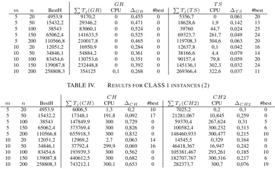
We define CLASS 0 the instances whereα = 0.75, CLASS 1 the instances where α = 1.00 and CLASS 2 the instances where α = 1.25. In this paper, we only report the results obtained with CLASS 1.

B. Results

We present in this section the computational results. In Table III, columnsm and n indicate the size of the instances, column ’BestH’ indicates the average best value, then for each heuristic algorithmH, one column indicates the average objective function valueP Tj(H), the average computation

time (in seconds), the number of times the method gives the best solution (#best) and the average deviation to the best solution∆.

∆H=

P Tj(H) − BestP Tj

P Tj(H)

GR indicates the greedy algorithm, T S refer to the Tabu Search algorithm with a Tabu list of 10 elements, andCH to the combined heuristic. The computation time has been limited to 300 seconds for all algorithms.

The results show the dominance of the Tabu Search. The Combined Heuristic CH is efficient for the small instances, with up to 50 jobs, but for larger instances, the CH2 with limited neighborhood is better.

VI. CONCLUSION

We approach a problem where am-machine permutation flow shop scheduling problem and a vehicle routing problem are integrated, and the objective is to minimize the total delivery tardiness. We present an MILP formulation of the problem, a greedy algorithm and Tabu Search based heuristics with an indirect coding for a solution. Some computational experiments are conducted and the first results show that the Tabu Search greatly improves the initial solution given byGR. In the future, it could be interesting to propose lower bounds for this problem. The scheduling problem and the

TABLE III. RESULTS FORCLASS 1INSTANCES(1)

GR T S

m n BestH P Tj(GR) CPU ∆GR #best P Tj(T S) CPU ∆T S #best

5 20 4953,9 9170,2 0 0,455 0 5356,7 0 0,061 20 5 50 15432,2 29346,2 0 0,471 0 18628,6 1,9 0,142 13 5 100 38543 83060,1 0 0,524 0 39760 44,7 0,024 25 5 150 65062,4 141633,5 0 0,525 0 69323,7 261,7 0,049 24 5 200 110566,8 210017,8 0 0,465 0 119708,3 304,6 0,063 20 10 20 12051,2 16950,9 0 0,284 0 12637,8 0,1 0,042 16 10 50 34846,1 54884,2 0 0,361 0 38166,6 4,4 0,079 14 10 100 83454,6 130753,6 0 0,351 0 90157,4 79,8 0,059 20 10 150 139087,8 232448,8 0 0,392 0 145136,1 302,3 0,032 24 10 200 258808,3 354125 0,1 0,268 0 269366,4 322,6 0,037 11

TABLE IV. RESULTS FORCLASS 1INSTANCES(2)

CH CH2

m n BestH P Tj(CH) CPU ∆CH #best P Tj(CH2) CPU ∆CH2 #best

5 20 4953,9 6006,5 1,3 0,2 10 7025,2 0,2 0,3 0 5 50 15432,2 17348,1 191,8 0,092 17 21281,067 10,845 0,259 0 5 100 38543 147849,9 300 0,729 0 59370,4 267,624 0,31 5 5 150 65062,4 373769,4 300 0,826 0 100582,4 300,232 0,313 6 5 200 110566,8 655918,3 300 0,832 0 148460,933 300,477 0,215 10 10 20 12051,2 12969,2 2,7 0,063 14 14545,5 0,329 0,164 0 10 50 34846,1 37792,4 299,9 0,069 16 46418,367 16,947 0,242 0 10 100 83454,6 193939,3 300 0,562 0 105381,467 293,261 0,185 10 10 150 139087,8 440612,5 300 0,682 0 182707,767 300,316 0,217 6 10 200 258808,3 743212,1 300,1 0,653 0 282373,7 300,7 0,076 19

vehicle routing problem being already difficult, finding good lower bounds seems to be very challenging. The resolution of the problem to optimality seems also to be a challenging problem. For this research direction, a model with less ’big-M ’ constraints can certainly be proposed, and decomposition methods seem to be research directions to investigate for such a difficult problem ([13]). Some other metaheuristic methods can be developed. A Tabu Search algorithm with a direct encoding can be proposed, as well as a genetic algorithm and a simulated annealing algorithm, known for its efficency for the two-machine scheduling problem. Then, the combination of mathematical programming and local search (matheuristic in the literature or hybrid optimization, see [6]) can be used, in order to improve the efficiency of the resolution methods. Hybrid methods seem very efficient for such difficult problems.

ACKNOWLEDGMENTS

This work was supported by the financial support of the Vietnamese government and by the ANR ATHENA project, grant ANR-13-BS02-0006 of the French Agence Nationale de la Recherche.

REFERENCES

[1] Armstrong, R., Gao, S., and Lei, L. A zero-inventory production and dis-tribution problem with a fixed customer sequence. Annals of Operations Research, 159(1), 395414, 2008.

[2] J.F. Bard, N. Nananukul, A branch-and-price algorithm for an integrated production and inventory routing problem. Computers and Operations Research 37:2202-2217, 2010.

[3] J-C. Billaut, T. Drevon, J-F. Tournamille, A complete view of the scheduling problem of chemotherapy production with expensive and perishable raw materials, 20th Conference of the International Federation of Operational Research Societies (IFORS2014), Barcelona, July 2014. [4] Campbell, H. G., Dudek, R. A., and Smith, M. L., A heuristic algorithm

for the n job, m machine sequencing problem. Management Science, 16(10):B630B637, 1970.

[5] Chen Z-L., Integrated Production and Outbound Distribution Scheduling: Review and Extensions Operations Research, 58(1), 130148, 2010.

[6] F. Della Croce and M. Ghirardi and R. Tadei, Recovering Beam Search:

enhancing the beam search approach for combinatorial optimization problems.Journal of Heuristics, 10:89–104, 2004.

[7] B. Fahimnia, R. Z. Farahani, R. Marian, L. Luong, A review and critique on integrated productiondistribution planning models and techniques Journal of manufacturing systems, 32(1):1-19, 2013.

[8] P. Farahani, M. Grunow, H-O. Gnther, Integrated production and dis-tribution planning for perishable food products. Flexible Services and Manufacturing Journal, 24:2851, 2012.

[9] F. Glover, Tabu Search - Part I. ORSA Journal on Computing, 1(3):1990– 206, 1989.

[10] F. Glover, Tabu Search - Part II. ORSA Journal on Computing, 2(1):4– 32, 1990.

[11] Hall, N. G., and Potts, C. N., Supply chain scheduling: batching and delivery. Operations Research, 51(4), 566584, 2003.

[12] Y. Kergosien, J-F. Tournamille, B. Laurence, J-C. Billaut, Planning and Tracking Chemotherapy Production for Cancer Treatment: a Performing and Integrated Solution, International Journal of Medical Informatics, vol. 80 (9), 655-662, 2011.

[13] Y. Kergosien, M. Gendreau, J-C. Billaut, A Benders decomposition based heuristic for a combined transportation and scheduling problem in chemotherapy production, Operational Research Applied to Health Services (ORAHS13), Istanbul, July 2013.

[14] Lee, C. Y., and Chen, Z. L., Machine scheduling with transportation considerations. Journal of Scheduling, 4, 324, 2001.

[15] J. K. Lenstra and A. H. G. Rinnooy Kan, Complexity of vehicle routing

and scheduling problems.Networks, 11,:221–227, 1981.

[16] Li, C. L., Vairaktarakis, G., Lee, C. Y., Machine scheduling with de-liveries to multiple customer locations. European Journal of Operational Research, 164(1), 39-51, 2005.

[17] A. Mazier, J-C. Billaut, J-F. Tournamille, Scheduling preparation of doses for a chemotherapy service, Annals of Operations Research, vol. 178 (1), pp. 145-154, 2010.

[18] Nawaz, M., Enscore, Jr, E. E., and Ham, I., A heuristic algorithm for the m-machine, n-job flow-shop sequencing problem. OMEGA, The International Journal of Management Science, 11(1):9195, 1983. [19] G. Steiner and R. Zhang, Approximation algorithms for minimizing the

total weighted number of late jobs with late deliveries in two-level supply chains. Journal of Scheduling, 12: 565574, 2012.

[20] E. Taillard, Some efficient heuristic methods for the sequencing prob-lem. European Journal of Operational Research, 47:65-74, 1990. [21] E. Vallada, R. Ruiz, and G. Minella, Minimising total tardiness in the

metaheuristics.Computers and Operations Research, 35(4):1350–1373, 2008.

[22] C. Virguz, S. Knust, Integrated production and sitribution scheduling with lifespan constraints. Annals of Operations Research, 213:293-318, 2014.

[23] C. C. Wu and W. C. Lee and T. Chen, Heuristic algorithms for solving

the maximum lateness scheduling problem with learning considerations.