Compartmentalization evaluated to explain discrepancies calculating cartilage fixed charge density

(1)

Compartmentalization Evaluated to Explain

Discrepancies Calculating Cartilage Fixed Charge

Density

by

Arun Mammen Thomas

S.B. Massachusetts Institute of Technology

Cambridge, Massachusetts (1995)

Submitted to the Department of Electrical Engineering and Computer

Science in Partial Fulfillment of the Requirements for the Degree of

Master of Engineering in Electrical Engineering and Computer Science

at the

MASSACHUSETTS INSTITUTE OF TECHNOLOGY

June 1998

@ Massachusetts Institute of Technology, 1998. All Rights Reserved.

Author:

_

Department of Electrical Engineering and Computer Science

May 26, 1998

Certified by:

Martha L. Gray

esh upervisor

s ,

-Accepted by:

Arthur C. Smith

Chairman, Department Committee on Graduate Theses

MASSACHUSETTS INSTITUTE

OF TECHNOLOGY

NOV 1 6 1998

LIBRARIES

(2)

(3)

Evaluation of Compartmentalization as an Explanation of

Discrepancies Calculating Fixed Charge Density in Cartilage

by

Arun Mammen Thomas

Submitted to the Department of Electrical Engineering and Computer Science June 30, 1998

In Partial Fulfillment of the Requirements for the Degree of Master of Engineering in Electrical Engineering and Computer Science

ABSTRACT

Recent studies on methods of detecting the early onset of arthritic cartilage degradation using NMR-based techniques have shown that such detection is possible. The use of sodium NMR observations, along with an ideal Donnan single compartment model of cartilage, has already been validated as a means of measuring cartilage fixed charge density - a known indicator of cartilage condition. Similar calculations of fixed charge density from proton (in the presence of gadopentetate) NMR observations and the same model were highly correlated with, but 50% below, values derived from sodium NMR. Maroudas had previously shown the water content of cartilage to be divided with a roughly 30:70 ratio between two physiologically distinct regions. The first of these regions, within cartilage collagen fibrils, is electroneutral, with most of the tissue fixed charge, in the form of chondroitin sulfate, being concentrated in the remainder of the tissue, the second region. The existence of two compartments, with different associated fixed charge densities, is shown, by spreadsheet computations and analysis of previously published data, to be a possible reason for the observed 50% discrepancy. High-concentration chondroitin sulfate solutions within dialysis tubing bags were equilibrated in solutions containing sodium and gadopentetate ions. This solution/tubing apparatus mimicked an ideal Donnan single compartment. MR measurements of the amounts of the two ions and calculations of fixed charge density in the solutions based on the measurements yielded the same 50% factor. Since this artificial model did not include any collagen, there were no compartmentalization effects due to structural factors. A similar single-compartment was done using a non-ionic contrast agent to test for steric exclusion based compartmentalization. Although MR measurements revealed a discrepancy in contrast agent distribution, the discrepancy was exactly opposite what should have been observed had steric exclusion been a factor. In summary, it seemed clear that compartmentalization of water (from either cartilage structure or from steric exclusion) was not primarily responsible for the observed 50% discrepancy. Another explanation must be found. Thesis Supervisors:

Deborah Burstein, Ph.D.

Associate Professor of Radiology Beth-Israel Hospital

Harvard Medical School Martha L. Gray, Ph.D.

J.W. Kieckhefer Professor of Electrical Engineering

Department of Electrical Engineering and Computer Science MIT and Harvard-MIT Division of Health Science and Technology

(4)

(5)

List of Figures

Figure 2.1: A cartoon sketch of cartilage structure depicting gray-banded collagen fibrils and black bottlebrush proteoglycans, the main constituents of cartilage. The white portions within the diagram should not be taken as empty, but rather, as filled with

water. Also found in this space are noncollagenous proteins, glycoproteins, and chondrocytes (not depicted because they are unimportant for the purposes of this w ork) ... ... 17 Figure 2.2: Collagen in the extracellular matrix. Three procollagen strands twine to form

a triple helix, which cross-links with other similar strands to form a microfibrillar bundle. The microfibrillar bundles then undergo further cross-linking with other bundles to form higher order structures (larger fibrils and fibers)... 18 Figure 2.3: Cartoon of a proteoglycan molecule, the other major component of the

cartilage extracellular matrix, marking the core protein and three distinct regions. For the purposes of this work, the focus will be primarily on the last region, the chondroitin sulfate, which is the main charge carrying material. Not shown here are the hyaluronic acid chains to which proteoglycans are bound, and the link proteins,

which connect the binding region to the acid. ... ... 19 Figure 2.4: The structural diagram of the chondroitin sulfate monomer is shown here. At

physiological pH, the monomer (MW = 459.39 g/mol) is ionized, with both the carboxyl and the sulfate groups maintaining a negative charge. ... 19 Figure 2.5: Spinning nucleus and associated magnetic moment. When a magnetic field is

applied, the magnetic moment of the nucleus begins to precess about an axis parallel to the applied field ... ... 25 Figure 2.6: Nuclei before and after a static magnetic field Bo is applied. (a) depicts the

random arrangement of the magnetic moments before application of the field. (b) shows the Bo field, and the resulting ordering of the magnetic moments into two groups, with one set pointing up (parallel spin) and the other pointing down (anti-parallel). The slight preponderance of those pointing up over those pointing down cause the generation of a cumulative magnetic moment M ... 27 Figure 2.7: Depicted here is the state of net magnetization immediately after the

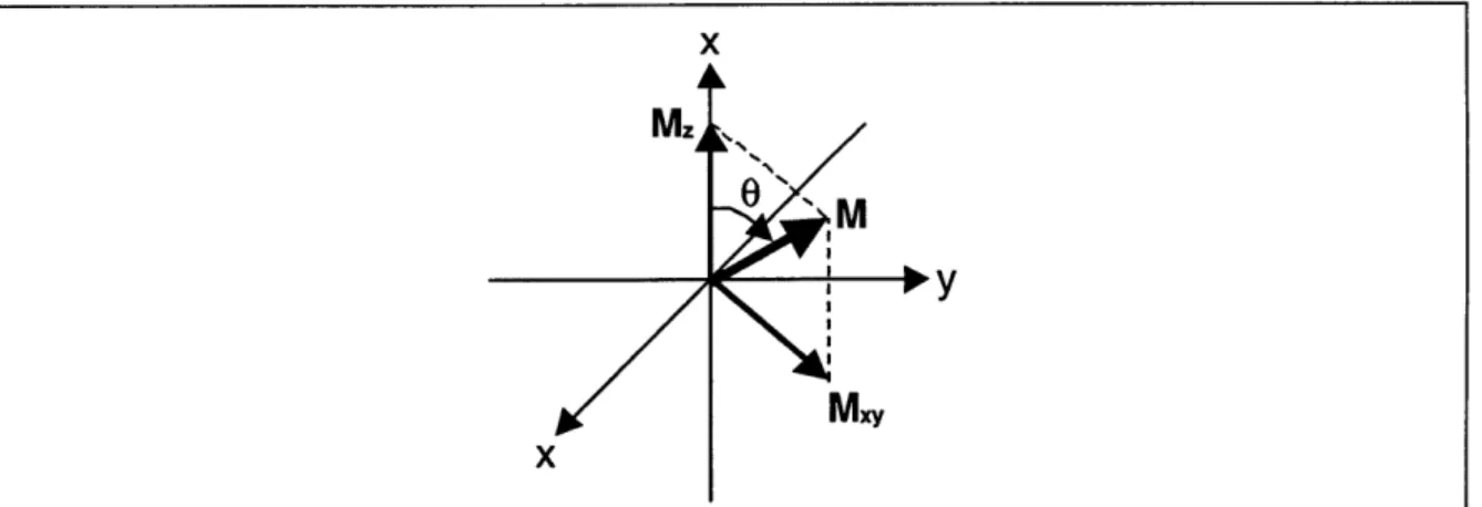
excitation pulse, B1, is turned off. M has been rotated away from the z-axis by an angle 0. Under the influence of the static magnetic field, it continues to precess about the z-axis which is collinear with the direction of Bo. This precession is

reflected in the xy plane by the rotation of the transverse component of M, Mxy. .... 28 Figure 2.8: The spin-spin relaxation time describes the rate at which transverse

magnetization, the detectable component of total magnetization, decays. Md is the initial (detectable) transverse magnetization immediately after excitation. ... 30

(8)

Figure 2.9: The spin-lattice relaxation time is associated with the renewal of the longitudinal component of the net magnetization vector. Here, Mo represents the magnitude of the net magnetization M at equilibrium (before any excitation has

taken place, or after the decay processes have been long completed) ... 30 Figure 2.10: T1 relaxation after a 1800 pulse occurs as shown here. Once again, Mo

represents the magnitude of the net magnetization M at equilibrium (before any excitation has taken place, or after the decay processes have been long completed).31 Figure 2.11: A chemical structural diagram of gadopentetate (Gd-DTPA-2_{). The zigzag}

line in the picture represents a temporary weak bond with a water molecule in the neighborhood of the gadopentetate ion. By binding in this manner, the water molecule is forced to spend more time in the vicinity of the magnetically active Gd-DTPA-2, which increases the relaxing effect. ... ... 34 Figure 2.12: This data in this graph (copied with permission of the author) was published

by Bashir et al in 1996 [7]. The x-axis is FCD as calculated from measurements of

Na concentration. The y-axis is FCD as calculated from measurements of Gd-DTPA-2 _{concentration. Both measurements were taken after equilibration in solution}

containing both sodium and gadopentetate. The slope of the regression fitted line shown is 0.49. The ideal Donnan model has no explanation for this factor of 2 difference in calculated values ... 35 Figure 3.1: Values for FCD as calculated from sodium are chosen. Each value is then

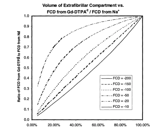
used to determine FCD as it would be calculated from gadopentetate, and the ratio of the two numbers is taken. This value is plotted versus the volume fraction of the total cartilage water content that is found within the extrafibrillar space. It was also assumed, plotting these curves, that bath concentrations of Na and Gd-DTPA-2 were 150mM and lmM respectively. Note that none of these curves are horizontal lines, showing that this ratio is, indeed, dependent on the volume of the extrafibrillar compartment. Further, all curves meet when 100% of the volume is extrafibrillar. At that point, an ideal single compartment exists. Although not shown here, the curve generated for an FCD of -300mM shows a ratio of 0.51 at 70% extrafibrillar w ater.... ... 39 Figure 3.2: Values for FCD as calculated from sodium are chosen. Each value is then

used to determine FCD as it would be calculated from chlorine, and the ratio of the two numbers is taken. This value is plotted versus the volume fraction of the total cartilage water content that is found within the extrafibrillar space. It was also assumed, plotting these curves, that bath concentrations of Na and C1- were 150mM. Note that none of these curves are horizontal lines, showing that this ratio is, indeed, dependent on the volume of the extrafibrillar compartment. Further, all curves meet when 100% of the volume is extrafibrillar. At that point, an ideal single

compartment exists. Qualitatively, these curves very much resemble those shown in

Figure 3.1 for G d-D TPA 2...42

(9)

Figure 3.3: A plot of FCDs as calculated from measurements of sodium concentration vs. FCDs as calculated from chlorine concentration. The slope of the regression line is

1.11, fairly close to the value expected if the system was well described as a single ideal Donnan com partm ent. ... 45

Figure 3.4: Values for FCD as calculated from sodium are chosen. Each value is then used to determine actual FCD in the extrafibrillar compartment. From this value, a volume averaged FCD is calculated, and its ratio to the originally chosen value is taken. This value is plotted versus the volume fraction of the total cartilage water content that is found within the extrafibrillar space. It was assumed, plotting these curves, that bath concentrations of Na+ 150mM. The largest differences between volume averaged FCD and FCD from sodium measurements occurs in the low FCD

region ... ... 46

Figure 4.1: Serial dilutions for making chondroitin sulfate solutions of different

concentrations. The first 100mg/ml solution was mixed up separately ... 50 Figure 4.2: Dialysis bag apparatus. Glass beaker, here depicted with only one sample,

can hold all six samples simultaneously. Each tubing apparatus floats marble side down in the equilibration solution. The tubing closures are lighter than water. Not only do the marbles help to weigh down each bag, but they also help to orient each

one vertically... ... ... 52 Figure 4.3: Serial dilutions for making Gd-DTPA-2 _{solutions of different concentrations.}

The first 50mM solution was mixed up separately ... 56 Figure 5.1: Plot of FCD as calculated from measurements of Na+ concentration against

FCD as calculated from measurements of Gd-DTPA-2 concentration. The data leading to these values of FCD were from NMR measurements of chondroitin sulfate solution that had been equilibrated in Hank's solution with Gd-DTPA2. Since there was no collagen present, the solution in dialysis bag construct should have been an ideal single compartment. Yet the regression line slope for these data is

approximately 0.468 rather than the expected value of one. ... 61 Figure 5.2: This graph plots FCD as calculated from measurements of Na+ concentration

against FCD as calculated from measurements of CS concentration via DMB. Unexpectedly, the slope of the regression curve here is 0.515. There is an apparent factor of two ratio between FCD from sodium and FCD from DMB. This lead to verification the Gd-DTPA-2 does not affect the DMB assay (Table 5.3). Ultimately, repetition of this particular comparison using data from other experiments refuted the suggestion that a factor of two ratio actually exists ... 62 Figure 5.3: Another plot of FCD as calculated from measurements of Na+ concentration

against FCD as calculated from measurements of Gd-DTPA-2 concentration. The data leading to these values of FCD were from a second set of NMR measurements of chondroitin sulfate solution that had been equilibrated in Hank's solution with

(10)

Gd-DTPA-2_{. The regression line slope for these data is approximately 0.5181. The}

factor of two relationship here remains as in the previous experiment. ... 64 Figure 5.4: A second plot of FCD from sodium measurements against FCD from the

DMB assay. Unlike the last time (Figure 5.2), the slope of the regression line is approximately equal to one, providing support for the idea that the previous set of measurements was somehow skewed by a factor of two during the experiment ... 65 Figure 5.5: This figure shows concentrations of sodium and ProHance in the dialysis bags normalized to concentrations outside. As expected from Donnan considerations, the concentration of sodium inside increases with respect to the outside as fixed charge density increases. At low FCDs, [ProHance] behaves exactly like a non-ionic material is expected to behave under Donnan equilibrium: the normalized

concentration is about equal to 1, and is fairly constant with fixed charge density. At higher FCDs, however, the ProHance concentration actually appears to increases in the sample. (Steric exclusion would suggest a decrease.) The "Disassociation Compensated" curve on the graph represents an attempt at explaining the apparent increase in sample [ProHance]. Disassociated Gd+3 could significantly alter the Tis used to calculate [ProHance]. The curve represents [ProHance] corrected for a 1% disassociation. ... 67 Figure 5.6: This graph plots FCD as calculated from measurements of Na concentration

against FCD as calculated from measurements of CS concentration via DMB. The observed slope of the regression line here is 1.09, very close to 1. ... 69 Figure 5.7: This graph, representing a fourth experiment, also depicts FCD from sodium

against FCD from the DMB assay. Here, although there is a greater spread of the points, the slope of the line is again near one (1), at 0.90 ... 70

(11)

List of Tables

Table 3.1: The data in the first four columns of this table is a collation of data gathered by Bashir using bovine cartilage samples. Note that all concentrations are in units of mM. Given ion concentrations in equilibrating solution as well as measured ion concentrations in the tissue, FCDs are calculated treating the tissue as a single homogenous compartment. As Bashir et al demonstrated [7], FCDs calculated in this manner from measurements of [Na+] and [Gd_DTPA-2] are unequal. The last column contains the relative volume fraction of the extrafibrillar compartment required to force sodium and gadopentetate measurements to give the same value for FCD in the extrafibrillar space. The average and standard deviation of these values are presented as well. These data seem to suggest that roughly 70% of the sample water was in the extrafibrillar space ... ... 40 Table 3.2: The data in the first five columns of this table is copied from data published by

Evans and Maroudas [52]. Note that all concentrations are in units of mM. Given ion concentrations in equilibrating solution as well as measured ion concentrations in the tissue, FCDs are calculated treating the tissue as a single homogenous

compartment. Interestingly, the calculated FCDs are sometimes fairly close to each other, and sometimes quite far apart. The last column contains the relative volume

fraction of the extrafibrillar compartment required to force sodium and chlorine measurements to give the same value for FCD in the extrafibrillar space. The average and standard deviation of these values are presented as well. The average value calculated here is actually greater than 1 (this is biased heavily by a single sample - sample 2 from subject age 67) which is impossible. Considering that quite a few of the individual samples also require an extrafibrillar volume fraction greater than one in order to set FCD from Na+ equal to FCD from C-, however, it seems clear that either the two compartment model does not well suit this data, or these data are inaccurate... ... 43 Table 5.1: Shown here are the FCDs, in moles/liter (M) of five cartilage samples both

before and after treatment with trypsin. Before the treatment, as expected form the results of Bashir et al [7], the average of the ratio between FCDs calculated from Na+ and from Gd-DTPA-2 is equal to 0.447 and is within one standard deviation of 0.5. After treatment, no attempt was made to evaluate the ratio. The calculated fixed charge densities were, for many of the samples, actually positive values, which clearly indicates difficulties with measurement... ... 58 Table 5.2: Gadopentetate concentration in the five cartilage samples after degradation by

trypsin was calculated from T1 measurements. The difference between tissue and bath concentrations is shown here in the last column. Note that the average difference, while not actually equal to zero, is more than an order of magnitude smaller than the concentrations involved ... ... 59

(12)

Table 5.3: Ratio of CS concentration measured via DMB to actual CS concentration. Although the [CS] calculated from DMB is at least 5% greater than the known [CS] of each sample, note that the same holds true for the OmM [Gd-DTPA-2] solution. This means that the 5% difference is likely to be measurement or calculation error, having no significance as far as the effect of gadopentetate upon the DMB assay. In fact the standard deviation for these samples is only 1% ... 63

(13)

Chapter 1: Introduction

Articular cartilage is a connective tissue found covering the surfaces of the bones in a joint. It provides a lubricated surface to permit smooth motion, and serves to harmlessly transfer load across the joint. Osteoarthritis is a degenerative disease of cartilage progressing from inflammation to eventual destruction of the tissue. It affects millions of people around the world. The United States, in particular, has cause for concern as the baby-boom generation reaches the age groups found to be most affected by arthritis. A 1992 study [77] (based on U.S. data collected between 1970 and 1987) showed that over 55% of those over 70 years of age were afflicted with arthritis. This makes the disease the number one concern for the elderly. The same study showed, however, that the elderly are not the only ones affected by this disease.

Although arthritis only affects a mere 5% of the working age adults - those between 18 and 64 years of age - the percentages shield the actual impact of disease. In fact, over 9 million of the working age adults in the United States reported having arthritis, and 5.5 million found their activities limited by the disease. The study continued on to show that arthritis had an obvious detrimental effect on the labor participation rate of those afflicted.

Clearly, arthritis is a disease with great relevance to the concerns of the nation and, indeed, to the individuals of that nation. It is also a disease that is currently not well understood. Preventive methods are primarily focused on eliminating risk factors derived from an understanding of the function of cartilage at a mechanical rather than a molecular level [64]. Current methods of diagnosis are based very much on reports of subjective symptoms such as stiffness, swelling, fatigue, tenderness, pain, etc. A generally accepted

(14)

quantitative method for identifying the disease has yet to be established. Visualization procedures for arthritis suffer from similar problems. Historically, visualization was via radiographs, which permitted only an indirect and clumsy assessment of cartilage condition by examining the space between the bones at a joint. More recently, arthography and computed tomography permitted better visualization, but even these invasive techniques were unable to identify arthritis prior to the appearance of gross structural changes.

Magnetic resonance imaging (MRI), a visualization technique developed from nuclear magnetic resonance (NMR), is an even more recent arrival in the visualization field. It has met with considerable success imaging cartilage as several techniques now exist to enhance the MRI contrast between different types of tissue. (The delineation between the hard - bone - and soft - cartilage - tissues of joints is particularly good.) Work has even been done to show that changes in cartilage thickness can be visualized using MRI, permitting replacement of the more traditional radiographic images [63].

Recent efforts have focused using NMR and MRI as non-invasive tools to quantitatively diagnose arthritis by attempting to detect pathologic indications of the disease state. One of the early signs of osteoarthritis, is the loss of one type of material, proteoglycan, from the tissue. Venn and Maroudas [72] showed that arthritic cartilage shows a significant reduction in proteoglycans as compared to normal cartilage. A means of measuring the proteoglycan content of cartilage, therefore, would provide a direct measure of tissue health. MR methods for diagnosing arthritis have focused on just such early detection of changes in cartilage proteoglycan content by making use of specific properties of the compound. Lesperance et al [47] showed that NMR measurements of

(15)

sodium content of in vitro samples can lead to a quantitative determination of proteoglycan content. Bashir et al's work [7] made use of the same principles to demonstrate that proton NMR in the presence of a specific MR contrast agent, gadopentetate dimeglumine, could be used for the same purpose. Recent work has further established that MRI in the presence of gadopentetate dimeglumine can distinguish arthritic cartilage from healthy human tissue and has suggested that in vivo monitoring of proteoglycan is possible [5,6].

Strangely, although the technique established by Bashir et al succeeds in tracking proteoglycan content, simultaneous measurements with sodium NMR and proton NMR yield quantitative values that differ by roughly a factor of two [7]. The goal of this work is to explore one hypothesis explaining the nature of this factor.

(16)

Chapter 2: Essential Background

2.1 Cartilage Physiology

There are many different cartilaginous tissues in the body. Nevertheless, all forms of cartilage share a gross similarity in their composition. Cartilage is a mostly cell-free tissue. The endogenous cells, known as chondrocytes, take up only about three to five percent of the tissue volume. They do not take an active role in the biomechanical role that cartilage plays but maintain, via synthesis, secretion, and degradation, an extracellular matrix (ECM) to fill that role [31]. The ECM provides mechanical strength via two main routes - electrical interactions due to ionic groups, and mechanical interaction due to chemical bonds between the structural elements of the matrix [19].

This extracellular matrix, the main part of cartilage tissue, is made up of water (65-80% of wet weight), collagen (15-25%), proteoglycans (3-10%), and various other noncollagenous proteins and glycoproteins [51]. Considering the relatively low concentration of noncollagenous proteins and glycoproteins present, cartilage can, for some purposes, be considered primarily a two-phase mixture of porous but insoluble collagen fibers and a solution of water and proteoglycans [19]. Figure 2.1 is a cartoon sketch of a segment of cartilage incorporating the two main non-water components, collagen and proteoglycan. These two elements will be the focus of the remainder of this section.

The collagen building block is a triple helix of procollagen chains, which link to each other via disulfide bonds during synthesis. The resulting collagen monomers, molecules about 300nm long, are arranged into arrays in which individual monomers again cross-link, forming microfibrillar bundles (Figure 2.2). Assembly continues as

(17)

bundles link to each other, leading eventually to the formation of a mature collagen fibril. The final strand can be quite long (as much as I4m) and can have a diameter ranging from 50 to 150nm depending on location [71]. This cross-linked collagen network provides the structural support upon which the ECM is built. It provides tensile strength, and limits swelling of the tissue from osmotic or hydrostatic pressures.

It is useful to note that although collagen molecules have chemical groups which ionize at physiological pH, those which are positively charged (amino, NH 3) are about

equal in number to those which have a negative charge (carboxyl, COO-). As a result, there is no net charge. This fact permits us to conclude below that collagen does not contribute to our MR measurements.

The other major non-water constituent of cartilage is the proteoglycans. The bottlebrush-like proteoglycans are usually found in large aggregates non-covalently inked

(18)

to hyaluronic acid chains. The binding of proteoglycan to acid is a complex process requiring a linking protein to join the binding region of the proteoglycan protein core to the acid. A proteoglycan is composed, as the name suggests, of a long protein core chain to which are attached other sugar compounds known as glycosaminoglycans (GAGs). In articular cartilage, these sugar compounds include disaccharide polymers, principally keratan sulfate (KS) and chondroitin sulfate (CS).

Figure 2.2: Collagen in the extracellular matrix. Three procollagen strands twine to form a triple helix, which cross-links with other similar strands to form a microfibrillar bundle. The microfibrillar bundles then undergo further cross-linking with other bundles to form higher order structures (larger fibrils and fibers).

Figure 2.3 shows a cartoon of one proteoglycan. A proteoglycan strand is known to have at least three different regions along the protein core [33]. One of these regions is particularly rich in bound keratin sulfate, while the other is rich in bound chondroitin sulfate. In general, the chondroitin sulfate is more plentiful not only because the CS polymers tend to be longer than the KS polymers, but also because the CS binding region is significantly larger, resulting in many more bound CS chains.

(19)

) Keratan Sulfate

i/

Binding Region Core Protein Chondroitin Sulfate

Figure 2.3: Cartoon of a proteoglycan molecule, the other major component of the cartilage extracellular matrix, marking the core protein and three distinct regions. For the purposes of this work, the focus will be primarily on the last region, the chondroitin sulfate, which is the main charge carrying material. Not shown here are the hyaluronic acid chains to which proteoglycans are bound, and the link proteins, which connect the binding region to the acid.

A structural diagram of the chondroitin sulfate monomer in both its neutral and ionized form is provided in Figure 2.4. At physiological pH, the disaccharide is ionized with both the carboxyl (COO-) and sulfate (S03-) groups negatively charged. Each

Figure 2.4: The structural diagram of the chondroitin sulfate monomer is shown here. At physiological pH, the monomer (MW = 459.39 g/mol) is ionized, with both the carboxyl and the sulfate groups maintaining a negative charge.

disaccharide, therefore, has a net -2 charge. Unlike unbound ions in the electrolytic fluid, which are free to diffuse in and out of the tissue, the charge on the chondroitin sulfate is

a /

1\

I

(20)

firmly "fixed" to the proteoglycans in the cartilage. As a result, the tissue is said to possess a fixed charge. In general, the concentration of fixed charge is referred to as the fixed charge density - FCD. (Although keratan sulfate has not been described specifically, it too is negatively charged at physiological pH - though only with a -1 charge per disaccharide [12] - contributing a component to the fixed charge density of cartilage.) The proteoglycans, because of their charge, become responsible for much of the stiffness and resilience of cartilage.

2.2 Donnan Based Derivation of FCD

The association of fixed charge with the proteoglycans on cartilage suggests that accurate determination of fixed charge density might act as a useful measure of the amount of proteoglycan in the tissue. (As has been noted previously, loss of proteoglycans is one of the early signs of the onset of arthritis.) One method of determining FCD, to be described here, makes use of measurements of mobile ion concentrations.

The presence of the fixed charge within the cartilage attracts mobile ions of opposite charge (counter-ions) and repels mobile ions of similar charge (co-ions). Therefore, although the tissue as a whole - solid and fluid components - has no net charge, an unequal distribution of mobile ions is set up between the tissue fluid and the external solution - which has no fixed charge. Since positive cations are preferentially attracted to the tissue while negative anions are repelled, the buildup of mobile charges sets up an electrical potential (the Donnan electrical potential) across the interface of the external solution and the cartilage. Distribution of ions obeys the Donnan equilibrium equation [51], which relates ion concentrations to the Donnan potential.

(21)

The ideal Donnan assumption states that electrolyte activity coefficients for ions are the same both in external solution and within any charged material, or, equivalently, that the ratio of electrolyte activities in external solution to electrolyte activities in charged material is equal to the ration of concentrations. This assumption, combined with some other approximations [30], leads to the following general expression:

Le RT

SCi )

Equation 2.1

where

Ci concentration of species i in charged material

Ci = concentration of species i in external solution Zi = charge on species i

T temperature

A1 Donnan potential

F Faraday's constant

R ideal gas constant

This relationship tells us that, at equilibrium, which implies no net flux of ions, given a constant temperature, the ratio of concentrations of any species of ion within and without a charged material is fixed to a constant value.

Another useful generalization deals with bulk electroneutrality. On a macroscopic scale, any given volume must satisfy electroneutrality, the sum of all the positive and negative charges within the volume must be zero. The following equations express this statement for two regions; the interior of a charged material, and the external solution.

(22)

ZCi+FCD = 0 Equation 2.2

SZi Ci = 0

Equation 2.3

Given these relationships, consider a sample of cartilage equilibrated in a solution with a relatively high concentration of NaCl (Na+ and Cl), and much smaller

concentrations of other minor ions (PO-3, CO-3, H+, Gd-DTPA-2_{). Applying Equation 2.1}

to some of the ions results in the expression below.

CNa+ C CI- C Gd-DTPA-2

CNa+ CCI- Gd-DTPA-2

Equation 2.4

This expression could be further extended to incorporate all the other ions present as well. The Gd-DTPA-2 ion was chosen here as an example for reasons that will become clear later in this work.

Application of Equation 2.2 and Equation 2.3 requires a little more thought. In general, it is difficult to be absolutely sure exactly which ions are present in solution. Certainly, the external solution surrounding cartilage in vivo contains a whole melange of ions which differ to some extent depending on the individual in question. A key approximation, however, makes these two equations simpler. The choice is to approximate as equal to zero the concentrations of those ions which are present only at relatively low concentrations. In the human body, most fluids contain relatively large concentrations of NaCI, and a few other ions. The majority of the ions found are present only at very low concentrations. For the example described above, Equation 2.2 and

(23)

CNa+ + cci- + FCD = 0 Equation 2.5

CNa+ + CcI_ =0

Equation 2.6

Note that here, only the Na and C1- ion need be considered, as all other ions are only present at relatively low concentrations.

Putting together Equation 2.4, Equation 2.5 and Equation 2.6, we can solve for fixed charge density in terms of the concentrations of various ions [7,47].

2 2 CCT CCr Cd-DTPA-2 Gd-DTPA 2 F C - = N C -2 Cc FCD- c a- + _ U CC1 = Gd-7DTPA Gd-DTPA-2

Na+ cI Gd-DTPA 2 Gd-DTPA

Equation 2.7

Some method of measuring ion concentrations, therefore, could lead directly to a value for FCD. (Note, however, that measurements of anion concentrations are much more likely to lead to errors in the values calculated for FCD. Since anions are preferentially repelled from the negatively charged material, the actual concentrations present are quite low. A fixed magnitude measurement error, therefore, will correspond to a greater relative error for anions than for cations.) In the work described here, ion concentrations are measured using NMR, and these measured values used to evaluate fixed charge density.

2.3 Nuclear Magnetic Resonance (NMR)

The magnetic resonance techniques used for the various measurements in this work have all been adequately described in the literature [7,22,23,47]. Nevertheless, a certain minimum exploration of some of the fundamental ideas behind NMR is called for at this point. An excellent quick reference (with very helpful graphics) for understanding

(24)

the basics of NMR physics, can be found on the world wide web on the Sheffield Hallam University School of Science and Mathematics web server [1]. Another slightly more detailed and ornate, but perhaps more useful web reference can be found at http://www.cis.rit.edu/htbooks/nmr [38]. Useful sources for more general information about NMR and MRI physics include particularly: Foundations of Medical Imaging by Cho, Jones and Shing [18], An Introduction to Magnetic Resonance by Carrington and McLachlan [17] and Magnetic Resonance Imaging edited by Partain. Finally, a very cogent overview of the mathematics behind MRI and NMR can be found in papers by Hinshaw et al [35], Sebastiani et al [70] and Mezrich [57].

2.3.1 Basic Principles

Atomic nuclei which contain an odd number of protons and/or neutrons possess a net magnetic moment t. These nuclei also possess angular velocity J related to the magnetic moment by Equation 2.8.

R=yJ Equation 2.8

y is the gyromagnetic ratio, a fundamental nuclear constant that differs for every

atomic element. In the absence of external magnetic fields, the magnetic moments are randomly oriented in space, and their vector sum is equal to zero. However, application of a magnetic field B results in a torque applied to the nucleus. Because the nucleus also has an angular momentum, J, the resulting motion is represented by:

dJ

(25)

Equation 2.9 simply states that the rate of change of angular momentum is determined by the applied torque. Joining this equation to Equation 2.8, gives the following interesting expression:

dt =y(gxB)

Equation 2.10

The magnetic moment changes in a direction perpendicular both to its direction and to the applied static magnetic field. Like a spinning top in a gravitational field, the magnetic moment begins to precess, as shown in Figure 2.5, around an axis parallel to the static field.

Applied magnetic field

Precessional orbit

Spinning

nucleus

Figure 2.5: Spinning nucleus and associated magnetic moment. When a magnetic field is applied, the magnetic moment of the nucleus begins to precess about an axis parallel to the applied field.

The frequency of precession (o in radians and f in Hertz), sometimes called the Larmor frequency, can be determined by solving Equation 2.10.

= 2f = y I B I

Equation 2.11

Quantum mechanics requires, in the presence of a static magnetic field Bo, that a particle with a magnetic moment be in one of a finite number of energy levels. The actual number of energy levels is determined by the spin quantum number I, another

(26)

intrinsic characteristic of the nucleus in question. The energies associated with each level are also a function of the spin and the magnetic field.

yhllBo hloo

E , -I = h l fo

2 2 =hfo

Equation 2.12

Note that the energy needed to move from one energy level to another is exactly the amount of energy stored in a photon at the Larmor frequency, hfo.

The number of nuclei populating each energy level is determined by Boltzmann statistics (Equation 2.13). At room temperature, although the thermal excitation is sufficient to keep the population levels just about equal, there is a slightly larger number of nuclei, some constant proportion of the total population, at the lower energy levels.

NH -AE/kT NL

Equation 2.13

NH= number of nuclei at higher energy level

NL, number of nuclei at lower energy level

AE ~-difference in energy between energy levels

T - temperature

k Boltzmann's constant

For a system with only two energy levels (1H), Figure 2.6 depicts the arrangement of the nuclei both before and after a static magnetic field is applied. The excess magnetic moments in the lower energy level with its associated orientation of spins leads to the formation of a net magnetization M along the direction of the static magnetic field Bo.

Magnetic resonance occurs when a radio frequency (RF) rotating magnetic field B1, applied at the Larmor frequency causes magnetic moments to flip between energy

states. As Equation 2.12 showed, any photons at the Larmor frequency have the correct amount of energy to cause switching between levels. Since, at equilibrium as just shown,

(27)

there is an excess of spins in the lower energy state, absorption of energy takes place as spins are promoted to the higher energy levels. The RF pulse also serves to bring the phases of the individual magnetic moments into a coherent relationship. From a macroscopic perspective, this leads to the net magnetization vector M rotating away from its equilibrium state and precessing about the direction of B1 with a frequency o given

by Equation 2.11. The direction of M is given in terms of the flip angle 0 = olt where t is the duration of the B1 pulse.

(a) (b)

Figure 2.6: Nuclei before and after a static magnetic field Bo is applied. (a) depicts the random arrangement of the magnetic moments before application of the field. (b) shows the Bo field, and the resulting ordering of the magnetic moments into two groups, with one set pointing up (parallel spin) and the other pointing down (anti-parallel). The slight preponderance of those pointing up over those pointing down cause the generation of a cumulative magnetic moment M.

Figure 2.7 depicts the state of the net magnetization immediately after the B1 field

is turned off. The deflected M continues to precess about the main Bo field as it slowly returns to equilibrium. The component of M in the transverse plane, M,y, acts to induce a current in a coil. The resulting exponentially decaying sinusoidal voltage is commonly referred to as free induction decay (FID). The FID constitutes the MR signal.

When more than one species of atom is involved, each type rotates at a different frequency, fo, changing the shape of the FID by contributing a component at the new

(28)

Mxy

Figure 2.7: Depicted here is the state of net magnetization immediately after the excitation pulse, B1, is turned off. M has been rotated away from the z-axis by an

angle 0. Under the influence of the static magnetic field, it continues to precess about the z-axis which is collinear with the direction of Bo. This precession is reflected in the xy plane by the rotation of the transverse component of M, Mxy. 2.3.2 Signal Intensity

The magnitude of the FID corresponds directly to the magnitude of Mxy. Immediately after the B1 pulse is switch off, the magnitude of Mxy is directly related, via

the flip angle 0, to the magnitude of the net magnetization M.

I Mxy I = I M I sin 0 Equation 2.14

The magnitude of M, in turn, is directly related to the total number of nuclei. By measuring the initial magnitude of the FID, therefore, and given some standards against which to compare, it is possible to determine the total number of nuclei present. Further,

according to Fourier theory, the area under the curve of the Fourier transform of a signal is equal to the initial magnitude of the FID. This means that a measure of the area under the Fourier transform of the FID can also serve as a measure of the number of nuclei present.

Measurements of nuclei-number via measurements of FID signal intensity can also be performed regardless of the number of different atomic elements that are present.

(29)

Since y is different for every element, at a given static field strength B0, each element

responds to a different excitation frequency. Only that portion of the total net magnetization due to the material of interest will respond to excitation at that frequency. Measurement of the FID, therefore, can theoretically be used to pick out the amounts of all magnetically active elements.

2.3.3 Relevant Time Constants

After excitation, the net magnetization vector M slowly returns toward its equilibrium state via a process called relaxation. Relaxation is characterized by two time constants T1 and T2. (Figure 2.9 and Figure 2.8.) These time constants depend on certain

chemical and physical characteristics of the nuclei of interest, as well as on the properties of neighboring nuclei (which may consist of other elements). Measurements of differences in these time constants, therefore, can contribute useful information about elements other than those being directly excited by the RF radiation.

The spin-spin relaxation time, T2, is the characteristic time associated with

transverse magnetization relaxation. T2 is quite important as it determines the amount of

time available for stimulating and recording the FID. Equation 2.15, sketched in Figure 2.8, shows the relationship between T2 and the transverse component (My)of the net

magnetization M.

Mx

=Md

e

(30)

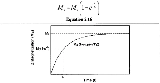
The spin-lattice relaxation time, TI, is the characteristic time associated with the regeneration of longitudinal magnetization, the z-component of M. Equation 2.16, sketched in Figure 2.9, shows the relationship between TI, and the longitudinal magnetization.

M =Mo 1-e

Equation 2.16 ~RM O -- -0 cis Mo (1-exp(-trT1)) SMo(1-e -1) ---N Time (t)

Figure 2.9: The spin-lattice relaxation time is associated with the renewal of the longitudinal component of the net magnetization vector. Here, Mo represents the magnitude of the net magnetization M at equilibrium (before any excitation has taken place, or after the decay processes have been long completed).

SMd 0 O (UI N ) C CC Mde-1 X Time (t)

Figure 2.8: The spin-spin relaxation time describes the rate at which magnetization, the detectable component of total magnetization, decays. initial (detectable) transverse magnetization immediately after excitation.

transverse Md is the

(31)

Interestingly, because of the physical process that cause relaxation, T2 is always

less than T1. This has the practical consequence of requiring a minimum recovery time

between excitations since the transverse magnetization will have vanished below the noise level before longitudinal magnetization has completely recovered.

Measurements of T1 are often made with what is known as an inversion recovery

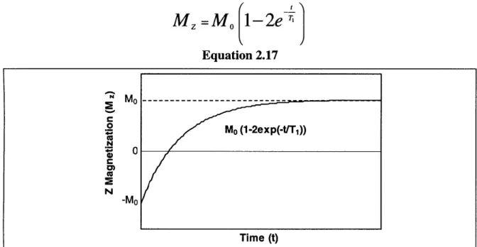
sequence. The flip angle 0 is initially chosen to be 1800 rather than the more usual 900. Once M is flipped by 1800, it has no transverse component. Recovery of the signal, sketched in Figure 2.10, proceeds as described by Equation 2.17.

M =

Mo-

2eT

Equation 2.17 M0 ---o Mo (1-2exp(-t/T1)) N 0 -Mo Time (t)

Figure 2.10: T1 relaxation after a 180' pulse occurs as shown here. Once again, Mo represents the magnitude of the net magnetization M at equilibrium (before any excitation has taken place, or after the decay processes have been long completed).

First applying a 1800 pulse, waiting a time r, and then applying a 90' pulse can identify specific points along this curve. The transverse magnetization after the second pulse will reflect the T1 relaxation that occurred during time r. After collecting several

points by choosing different values of t, a curve fit to an equation of the form of Equation

(32)

2.3.4 Contrast Agents

Contrast agents (so called because they can affect the contrast in MRI images) work by providing an extra source of magnetically active elements in solution so that relaxation can proceed faster. As the concentration of the contrast agent increases, the time constants decrease - relaxation happens faster. In general, the effect of contrast agent C on relaxation time constant T (the effect is applicable to both T1 and T2) is

described by Equation 2.18 [84].

R[C]= 1 1

Tc To

Equation 2.18

where

Tc - value of the relaxation time constant in the presence of C. T_oa standard value of the relaxation time constant.

R relaxivity of C.

[C] - concentration of contrast agent C.

The relaxivity, R, is a value that characterizes the efficiency with which the contrast agent increases water relaxation - decreases the time constant. It is important to note that since a particular contrast agent can affect T1 and T2 differently, the value of R

can be different depending on the time constant in question. For a novel contrast agent, R can be calculated simply by measuring the effect, on the time constant of interest, of various concentrations of the contrast agent - one of those concentrations, of course, will be 0 M, in order to provide a value for To. Having calculated the value of R from solutions of known concentration, the concentration of C in unknown solutions can be determined by measuring one of the time constants.

(33)

2.4 Previous Work

The use of NMR/MRI to examine cartilage has been a topic in the literature for some time [4, 7, 29, 36, 47, 62, 39]. The non-invasive nature of MR as well as its marked ability to effectively image soft tissues, combined with the prevalence of cartilage diseases makes the combination quite appealing. Some of the work that has been done, however, is of particular importance for this work, as the experiments described below

focus on particular aspects of this work.

2.4.1 Measurements with Sodium and Gadolinium

In 1992, Lesperance et al showed that NMR measurements of sodium ion concentration could be used to track tissue fixed charge density in cartilage via the Donnan model [47]. That paper also established that not only did sodium measurements track cartilage FCD, but the values so calculated were closely matched by values obtained by spectrophotometric assay methods. (Using bovine chondroitin sulfate as a standard led to a values of FCD that were 100 + 7% of those calculated from sodium concentration measurements.) Bashir further explored the possibilities by looking at the implications of sodium T1 and T2 for imaging [4]. Unfortunately, not only is sodium MR

complicated by extremely small T2s, but the amount of sodium present in organic tissues

is insufficient to provide a strong signal without repeating the scans many times for signal averaging purposes. Further, although sodium is ubiquitous in real physiological systems,

in vivo studies using sodium MR are impractical. There is currently no means of

quantifying the results of an in vivo sodium scan because of the interrelationship between the changing T2s and the observed sodium signal. On the other hand, if sodium

(34)

concentrations could be measured quantitatively, that same ubiquity would make sodium measurement quite attractive despite its other problems.

Ionic contrast agent gadopentetate, Gd-DTPA-2 (Figure 2.11) [11], an FDA

approved compound, is regularly used via injection in MRI studies. As such, there was information available on its use in other tissues [21] and its characteristics had been explored to some extent. [22].

H1O%0H

- -2

O O _-2

0Y

Figure 2.11: A chemical structural diagram of gadopentetate (Gd-DTPA'2). The zigzag line in the picture represents a temporary weak bond with a water molecule in the neighborhood of the gadopentetate ion. By binding in this manner, the water molecule is forced to spend more time in the vicinity of the magnetically active Gd-DTPA 2, which increases the relaxing effect.

In 1996, Bashir et al used measures of Gd-DTPA-2 in cartilage and Donnan theory to determine FCD [7]. They showed that, as with calculations using Na and calculations using Gd-DTPA-2 _{resulted in values of FCD that correlated very nicely (r}2_=0.94).

2.4.2 Effects of Particular Interest

Figure 2.12 is a copy of a graph published by Bashir et al. Note that the x and y axis both represent FCD. The only difference is that along the x-axis, FCD was calculated by measuring sodium concentration and applying the Donnan model. Along the Y-axis, on the other hand, FCD was calculated from measurements of gadopentetate

(35)

concentration. If the Donnan model adequately describes ion distribution, then the values calculated from the two measurements will be equal. However, this is not the case. In fact, the gadopentetate based values are related to the sodium based values by a line with a slope of 0.49 = V2. The goal of this work will be to examine one possible reason for this factor of two (or factor of one-half, depending on the viewpoint).

FCD from Na* vs. FCD from Gd-DTPA"2 -310 O Trypsh Seres -260 - Inte~ukh -1 Sexres Regmssbn Lhe M'-210 E i-" -160 E 0 0 U. -110

0

_oo

o

-60 o o o y= 0.491x- 8.2591 R2 = 0.9429 o0 O -10 o -10 -60 -110 -160 -210 -260 FCD from Na (mM) -310

Figure 2.12: This data in this graph (copied with permission of the author) was published by Bashir et al in 1996 [7]. The x-axis is FCD as calculated from measurements of Na' concentration. The y-axis is FCD as calculated from measurements of Gd-DTPA"2 concentration. Both measurements were taken after equilibration in solution containing both sodium and gadopentetate. The slope of the regression fitted line shown is 0.49. The ideal Donnan model has no explanation for this factor of 2 difference in calculated values.

(36)

Chapter 3: Theoretical Analysis

The structure of cartilage provides one possible explanation for the factor of two ratio noticed in Bashir's experiments [7]. As Figure 2.1 suggests, the water content of cartilage is divided between two different regions: the intrafibrillar region, within the collagen fibrils, and the extrafibrillar region. In fact, roughly 30% of the tissue water can be found within the collagen fibers [51]. The important aspect of this division, however, is the fact that, due to the networked structure of the collagen bundles, the proteoglycans (and therefore the associated fixed charge) cannot enter the collagen fibers [55]. This means that the two water populations, intra- and extrafibrillar, have different local fixed charge densities. Although the relationships outlined by Equation 2.1, Equation 2.2, and Equation 2.3 hold for each of the two regions, if compartmentalization is a factor, the relationships cannot be applied to the overall bulk of a cartilage sample.

The NMR methods developed by Lesperance et al [47] and Bashir et al [7], however, do not differentiate between the two water compartments. The values for sodium concentration and gadopentetate concentration calculated from NMR measurements reflect the volume averaged concentrations from each compartment.

C , = C IF, VIF + C EF, VEF

Equation 3.1

where

CM,- volume averaged concentration of species i (measureable)

VIF volume fraction of water in intrafibrillar space.

CIF, concentration of species i in intrafibrillar space. VEF - volume fraction of water in extrafibrillar space. CEF, concentration of species i in extrafibrillar space.

(37)

Since VIF and VEF are volume fractions, the following relation must hold true:

VIF + VEF = 1

Equation 3.2

Further, since the intrafibrillar space is charge free, at equilibrium, the concentrations of all ions within must be equal to the concentrations in the external solution. Only the concentrations of ions in the extrafibrillar space are affected by the fixed charge. In keeping with the notation introduced with Equation 2.1:

*.VIF 1-VEF

CIF, =Ci

CEF- i

Equation 3.1 can now be restated.

CM , C, -vEF)+ iCEF

Equation 3.3

3.1 Gd-DTPA

"2

_{Based Calculations}

Equation 3.3 provides the means to determine whether it is worthwhile to continue with this avenue of exploration. Spreadsheet based manipulations can provide an idea as to whether or not the partitioning of tissue water into two compartments has a significant effect on the ratio of FCD as calculated from measurements of Na and Gd-DTPA-2_{. Since measured concentrations are, in fact, the volume averaged concentrations}

of ions in the two compartments that compose cartilage, the fixed charge densities calculated using these measurements and the Donnan single compartment model must reflect the nature of the volume averaging. In fact, it is expected that FCD calculated from different ions will reflect volume averaging differently. Choosing a value to be the FCD as determined from Na+, and working backward using Equation 2.1, Equation 2.2,

(38)

Equation 2.3 and Equation 3.3, a value for FCD as it would be calculated from Gd-DTPA-2 _{can be derived. (This derivation is outlined in Appendix A.) Figure 3.1 plots the}

ratio of the two FCDs as a function of volume fraction of the extrafibrillar compartment, showing the effect of the presence of two compartments on calculations of FCD using a single compartment Donnan model and measurements of Gd-DTPA-2 and Na

concentrations.

All the curves in the figure have a non-zero slope. The ratio of FCDs does depend on the volume of the extrafibrillar compartment in this simulation, which makes it possible that the ratio observed by Bashir et al [7] can be explained as due to the existence of two distinct water populations within cartilage. Further, healthy cartilage is composed of roughly 60mg/ml chondroitin sulfate and has a fixed charge density between -200 and -300mM. In this range, a ratio of 0.5 between FCD from Gd-DTPA-2 and Na occurs for an extrafibrillar water content between 60 and 70%.

Table 3.1 contains data collected by Bashir. In the first four columns, the measured concentrations of sodium and gadopentetate in several samples under various bath conditions are marked down. Given these concentrations, FCD is calculated under the assumption that cartilage is a homogenous single compartment. As expected, the two values of FCD are unequal. Most of these data points appear in Figure 2.12 which shows the slope of the regression relationship between FCD calculated from Na and FCD calculated from Gd-DTPA-2 as being equal to about 0.5. The last column of Table

3.1 contains values for the volume of extrafibrillar water needed in order for a two compartment model to correctly explain the measured values. As shown in Appendix B, given the assumptions behind Equation 3.3, it is possible to derive the extrafibrillar

(39)

compartment volume fraction from measured tissue ion concentrations and known bath concentrations. Only one such volume will permit Donnan equilibrium to hold.

Volume of Extrafibrillar Compartment vs. FCD from Gd-DTPA 2 _/_{FCD from Na}

1.0 .. 0.9 " E 0.8 - Fo / 0 4 0 _ u. / 4 z -I-o -0.7 / 0.0 O i . ,-Ec 0.6 . / 4 to _o _0.5 _M _,'r " v ". sl do 1 0.4 / - FCD =-200 * / h t l , _o,i/ t _,t _FCD₌_-150 0.1_0.2 n- ₀.- - -FCD _{FCD = -10}= -20 0.0 .... 0.00% 20.00% 40.00% 60.00% 80.00% 100.00%

Volume of Extrafibrillar Compartment Relative to Total Volume

Figure 3.1: Values for FCD as calculated from sodium are chosen. Each value is

then used to determine FCD as it would be calculated from gadopentetate, and the

ratio of the two numbers is taken. This value is plotted versus the volume fraction of the total cartilage water content that is found within the extrafibrillar space. It was also assumed, plotting these curves, that bath concentrations of Na and

Gd-DTPA"2 were 150mM and 1mM respectively. Note that none of these curves are

horizontal lines, showing that this ratio is, indeed, dependent on the volume of the extrafibrillar compartment. Further, all curves meet when 100% of the volume is extrafibrillar. At that point, an ideal single compartment exists. Although not

shown here, the curve generated for an FCD of -300mM shows a ratio of 0.51 at

(40)

2 2 [Gd-DTPA 2] _{[Na ] in} in Bath Tissue C1 C2 C3 C4 C5 C6 C7 C8 150.0 150.0 150.0 150.0 150.0 150.0 150.0 150.0 150.4 150.4 150.4 150.4 150.4 150.4 150.4 150.4 150.4 150.4 150.4 150.4 150.4 150.4 150.4 [Gd-DTPA2 ] in Tissue 1.000 1.000 1.000 1.000 1.000 1.000 1.000 1.000 0.500 0.500 0.500 0.500 0.500 1.000 1.000 1.000 1.000 1.000 2.000 2.000 2.000 2.000 2.000 FCD from [Na1] 271.1 298.4 285.5 331.0 328.1 326.8 382.7 327.5 325.0 345.0 393.3 417.8 449.3 323.4 340.3 390.2 418.9 424.8 328.7 345.7 384.4 405.3 431.0 FCD from [Gd-DTPA 2] 0.550 0.470 0.480 0.420 0.420 0.420 0.330 0.440 0.168 0.178 0.122 0.120 0.125 0.348 0.312 0.271 0.269 0.241 0.825 0.733 0.612 0.558 0.572 Extrafibrillar Compartment Volume Fraction -188.1 -223.0 -206.7 -263.0 -259.6 -257.9 -323.9 -258.8 -255.4 -279.4 -335.8 -363.7 -399.0 -253.5 -273.8 -332.2 -364.9 -371.6 -259.9 -280.2 -325.5 -349.4 -378.5

Average of Extrafibrillar Compartment Volume Fraction: 0.7425 Std. Dev. of Extrafibrillar Compartment Volume Fraction: 0.0888

Table 3.1: The data in the first four columns of this table is a collation of data gathered by Bashir using bovine cartilage samples. Note that all concentrations are in units of mM. Given ion concentrations in equilibrating solution as well as measured ion concentrations in the tissue, FCDs are calculated treating the tissue as a single homogenous compartment. As Bashir et al demonstrated [7], FCDs calculated in this manner from measurements of [Na+] and [Gd_DTPA-2] are unequal. The last column contains the relative volume fraction of the extrafibrillar compartment required to force sodium and gadopentetate measurements to give the same value for FCD in the extrafibrillar space. The average and standard deviation of these values are presented as well. These data seem to suggest that roughly 70% of the sample water was in the extrafibrillar space.

As can be seen, most of the samples listed here would satisfy Donnan and have a volume averaged tissue concentration equal to the measurements if about 70% of tissue water was extrafibrillar. In fact, as the calculations at the bottom of the table show, the average required volume was 74%, with a standard deviation of 9%. The 70% value

Sample Name -91.0 -116.0 -112.6 -134.2 -134.2 -134.2 -174.9 -126.6 -172.4 -162.0 -230.5 -233.6 -225.6 -166.4 -185.4 -210.8 -212.0 -232.6 -137.6 -157.4 -188.7 -205.4 -200.7 [Na+ ] in Bath 0.535 0.623 0.624 0.664 0.666 0.667 0.750 0.638 0.796 0.742 0.860 0.849 0.820 0.780 0.813 0.825 0.810 0.843 0.677 0.727 0.781 0.805 0.782 _ _

(41)

derived here also agrees with values reported by Maroudas for valuations of water content of the extrafibrillar space. [51].

3.2 CI' Based Calculations

Having shown that the one to two ratio observed can theoretically be described by utilizing a two compartment model of cartilage, it was decided to determine if the same effect would be observed for calculations of FCD using measurements of chlorine ion concentration. The first step, once again, was to work backward from a chosen value of FCD as calculated from Na+ .

Using Equation 2.1, Equation 2.2, Equation 2.3 and Equation 3.3, the FCD as it would be calculated from Cl measurements can be found (Appendix A). Figure 3.2 plots the ratio of these two FCDs against the relative volume of the extrafibrillar compartment, showing the effect of the presence of two compartments on calculations of FCD using a single compartment Donnan model and measurements of Cl- and Na+ concentrations.

In order to examine this theoretical finding, the literature provides a source of experimental data. In 1972, Evans and Maroudas published a paper [52] describing research in which they made use of radiotracer methods to measure the concentrations of Na and Cl- ions in cartilage after it was allowed to equilibrate in solutions of known concentrations. Along with the relevant analysis, this paper included much of the raw data that was collected. Table 3.2 tabulate part of this data in the first 5 columns. (The first two columns simply identify the different samples.) For space reasons, several samples that were not used for the purposes of this paper were not included in the table. These samples were ignored for one of two reasons. In some cases, the data published contained what appeared to be typographical errors, as the values appeared to be a factor

Compartmentalization evaluated to explain discrepancies calculating cartilage fixed charge density