Comparison of PSF fitting methods for determining centroids of stars

COMPARISON OF

PSF

BY

STEPHANIE GIBSON

A THESIS SUBMITTED TO THE MASSACHUSETTS INSTITUTE OF TECHNOLOGY IN CONFORMITY WITH THE REQUIREMENTS FOR THE DEGREE OF BACHELOR OF SCIENCE.

CAMBRIDGE, MASSACHUSETTS

MAY 22, 2013 -

2

\3

@2013 STEPHANIE GIBSON. ALL RIGHTS RESERVED.

MASSACHUSETTS INSTITUTE OF TECHNOLOGY

SEP 28

2017

LIBRARIES

THE AUTHOR HEREBY GRANTS TO M.I.T. PERMISSION TO REPRODUCE AND DISTRIBUTE PUBLICLY PAPER AND ELECTRONIC COPIES OF THIS THESIS AND TO GRANT

OTHERS THE RIGHT TO DO SO.

AUTHOR SIGNATURE:

The uthor htrcby grants t0 MT peniss&On to

reDroduce and to distdibutl pubcly paper &nd lect-oroic _{copies of t thosis document in}

whol or in part in any medium nw known or h0rea ter crea d.

CERTIFIED BY:

Signature redacted

DEPARTMENT OF EARTH, ATMOSPHERIC, AND PLANETARY SCIENCES

MAY 22, 2013

Signature redacted

PROFESSOR RICHARD P. BINZEL THESIS ADVISOR

ACCEPTED BY:

Signature redacted

PROFESSOR RICHARD P. BINZEL

COMPARISON OF

PSF

BY

STEPHANIE GIBSON

SUBMITTED TO THE DEPARTMENT OF EARTH, ATMOSPHERIC AND PLANETARY SCIENCE ON MAY 22, 2013, IN PARTIAL FULFILLMENT OF THE REQUIREMENTS FOR THE DEGREE OF BACHELOR OF SCIENCE IN EARTH, ATMOSPHERIC AND PLANETARY

SCIENCE.

Abstract

This paper shows a comparison of four fitting models used in order to cal-culate the centroids for twelve stars. The offsets for each coordinate are calculated with respect to the mean of the coordinates for varying aperture sizes. The computed offsets are then compared to determine if there was any effect from the magnitude of the star or the star's position on the CCD

chip. An appropriate aperture size of 12 pixels is chosen in order to com-pare each method. It is determined that a magnitude effect exists, though it is very small and results in an approximate difference between residuals of between 0.02 and 0.04 pixels, which for most methods is within the fitting error. For the position on the chip effect, the vectors of the x and y residuals are produced in vector plots in order to demonstrate the directional tendency each fitting method had dependent on chip position. Each model has some dependency on position on the CCD chip, with 0.033 pixels as the largest variation between models. Therefore, for accuracy less than 0.033 pixels any of these models can be used for fitting a PSF to a star. However, if greater accuracy is needed more steps need to be taken in order to determine the best PSF fit.

Thesis Advisor: Richard P. Binzel

Contents

List of Tables

1 Circular Gaussian Fitting Errors . . . 24 2 Lorentz Fitting Errors . . . . 25 3 Elliptical Gaussian Fitting Errors . . . 25 4 Average Difference from Combined Mean for Fitting Methods 26 5 X Coordinate Offsets from Combined Mean for Fitting Methods 26 6 Y Coordinate Offsets from Combined Mean for Fitting Methods 27

List of Figures

1 Shape of Moffat Function Plotted . . . . 11 2 Shape of Gaussian Function Plotted . . . . 12 3 Shape of Lorentz Function Plotted . . . 13 4 Lorentz, Moffat, and Gaussian functions plotted together. Each

function plotted is normalized to have an area of 1, and this plot shows the difference in the wings of each function which is ultimately what determines which model is a better fit for

a star. ... . . . ... . . .. .. . . . .. . . 14 5 Star field image taken at Wallace Astrophysical Observatory

on a 14" telescope with a SBIG STL-1001E with an exposure time of 60 seconds and an image scale of 1.2 arc sec/pixel. The stars used for the PSF model comparison are circled. . . . . . 15 6 x-coordinate offset from the mean of x-coordinates for varying

aperture sizes. This plot was used in order to determine the best aperture size to use for model comparison, the least vari-ation occurs for aperture sizes between 10 and 15 pixels and so an aperture size of 12 pixels is chosen. . . . 19 7 Illustration of amount of PSF detected for a given aperture size 20 8 x-coordinate offset from the combined mean of x-coordinates

for a smaller subset aperture sizes. The least variation occurs for aperture sizes of 12 and 13 pixels, and so an aperture size of 12 pixels was chosen for the model comparisons. . . . 21 9 x-coordinate offset from the combined mean of x-coordinates

for a smaller subset aperture sizes scaled to the same y range as the full x-offset plot to show the lack of variation from the m ean . . . . 22 10 Radial profile of a star with a cutoff at a 12 pixel radius. All of

the fast-varying core of the star is included within this radius, along with a portion of the wings. . . . 23 11 Circular Gaussian x coordinate offsets for stars between 12.88

and 15.87 magnitude. Though outliers exist for stars of high magnitude and very small aperture sizes, there is a much smaller dispersion from the mean than for the Elliptical Gaus-sian and Moffat models, suggesting this model does not depend as much on aperture size . . . 28

12 Circular Gaussian y coordinate offsets for stars between 12.88 and 15.87 magnitude. Though outliers exist for stars of low magnitude and very small aperture sizes, there is a much smaller dispersion from the mean than for the Elliptical Gaus-sian and Moffat models, suggesting this model does not depend as much on aperture size . . . 29 13 Lorentz x coordinate offsets for stars between 12.88 and 15.87

magnitude. Though outliers exist for stars of low magnitude and very small aperture sizes, there is a much smaller disper-sion from the mean than for the Elliptical Gaussian and Mof-fat models, suggesting this model does not depend as much on aperture size. . . . . 30 14 Lorentz y coordinate offsets for stars between 12.88 and 15.87

magnitude. Though outliers exist for stars of low magnitude and very small aperture sizes, there is a much smaller disper-sion from the mean than for the Elliptical Gaussian and Mof-fat models, suggesting this model does not depend as much on aperture size. . . . . 31 15 Elliptical Gaussian x coordinate offsets for stars between 12.88

and 15.87 magnitude. The large spread from the mean over varying aperture sizes suggests that this model depends more on the aperture size than the Lorentz or Circular Gaussian m odels . . . . 32 16 Elliptical Gaussian y coordinate offsets for stars between 12.88

and 15.87 magnitude. The large spread from the mean over varying aperture sizes suggests that this model depends more on the aperture size than the Lorentz or Circular Gaussian m odels . . . 33 17 Moffat x coordinate offsets for stars between 12.88 and 15.87

magnitude. The large spread from the mean over varying ture sizes suggests that this model depends more on the aper-ture size than the Lorentz or Circular Gaussian models. . . .. 34 18 Moffat y coordinate offsets for stars between 12.88 and 15.87

magnitude. The large spread from the mean over varying ture sizes suggests that this model depends more on the aper-ture size than the Lorentz or Circular Gaussian models. . . . . 35

19 y coordinate offsets for Lorentz and Gaussian models plot-ted to the same scale showing that there appears to be less deviation from the mean than when viewed from different scales. The IRAF models appear to have the greatest disper-sion around the mean, but the Lorentz and Circular Gaussian

models had the greatest outliers for small aperture sizes. . . . 36

20 y coordinate offsets for the IRAF Moffat and Elliptical Gaus-sian models plotted to the same scale showing that there ap-pears to be less deviation from the mean than when viewed from different scales. The IRAF models appear to have the greatest dispersion around the mean, but the Lorentz and Cir-cular Gaussian models had the greatest outliers for small aper-ture sizes. . . . 36 21 x coordinate offsets for the the four models plotted to the same

scale showing that there appears to be less deviation from the mean than when viewed from different scales. . . . 37 22 x-coordinate offsets for stars of varying magnitudes calculated

from the combined mean of each method. It can be seen that a magnitude effect exists, especially for very high magnitudes with a difference of 0.06 pixels for a magnitude of 15.87, but that it is only apparent for magnitudes greater than 15. . . . . 38 23 Vector representation of x and y residual offsets for each method

scaled by 10. It appears that each method has some depen-dence on position on the CCD chip which most likely has to do with each star's orientation on the optical axis. . . . 40 24 Magnitude effect on vectors of residual offsets for each method.

Brighter stars are represented by yellow, darker stars by green with 12.88 as the lowest magnitude and 15.87 as the highest m agnitude. . . . . 42 25 Mathematica functions written to calculate X and Y center

Acknowledgements

I would like to thank Amanda Bosh for her tremendous help in every aspect of my paper, without whom this thesis would not be possible. I would also like to thank Jane Connor for her help providing guidance in the writing of my thesis. I would also like to thank Jessica Ruprecht and Rachel Bowens-Rubin for driving me to Wallace Astrophysical Observatory and offering help whenever I asked for it. Lastly, I would like to thank my thesis advisor Rick Binzel for always leaving his door open to me if I had any concerns whatsoever.

Introduction

Determining the geometric centers (centroids) of stars lies at the heart of all astrometric calculations because accurate position determination is crucial for studying the movements of celestial bodies. Though stars are considered point sources due to their distance from the Earth, the profiles of stars viewed from the ground imaged onto two-dimensional arrays are point-spread func-tions (PSFs) due to the effects of the turbulent mixing of the atmosphere (known to astronomers as seeing). The PSF is the spatial distribution of the intensity of the star, and these distributions can be modeled by several dif-ferent functions. These profiles usually have large wings that decrease as an inverse square of intensity, and so can be modeled by Gaussian, Lorentzian, or Moffat functions.

The motivation of this paper is to determine to what degree PSF fitting models affect the center calculations of stars, and whether certain models are superior for fitting PSFs for stars of varying magnitudes. It is important to find each model's strength in calculating the centers of stars because accurate center calculations are crucial to all astrometric calculations.

Given that the star image is spread out across several pixels, a precise meaning must be given to the coordinates of the star. The coordinates of a star are chosen to be the centroid, and so it is important to determine this position to the greatest accuracy and precision. Merely clicking on the location of a star's maximum intensity on a charge-coupled device (CCD)

frame will only yield precision to one pixel, and so alternative methods must be employed in order to obtain sub-pixel (at least on the order of .01 pixel) precision.

The approximate functions for the various methods are as follows.

Moffat

A typical Moffat function as described by Trjuillo et al. (2001), is

PSF(r) = 21+ , (1)

7T a2

with the full width at half maximum, FWHM=2a21/_1 - 1. The parameter a is then determined by the formula

FWHM (2)

2 270- 1

where the variable r is the radial distance. The Image Reduction and Anal-ysis Facility (IRAF) software uses a simplified version of this function and is described in the Methods section. The Moffat function is a popular PSF model for stars because of its prominent and extended wings which closely resemble star images, Noel (2006).

Moffat Function

--10 -5 0 5

r

Figure 1: Shape of Moffat Function Plotted

Gaussian

The Gaussian model for a PSF is a limiting case of the Moffat PSF (when

#

PSF(r) = 4 (21/ - 1)

wF

1 +4(21/3-3 1)2 (3)

As 3 -+ oc, we can substitute 21/1 - 1 with (In 2)/0, so:

lim PSF(r) = lim 3-141n2 340 13-00

3

+

lim PSF(r) = 2 2 e

'3-+o0

27ro-where the parameter a is the standard deviation of the data.

U-C', a. 0.07 0.06 0.05 0.04 0.03 0.02 0.01 0.00 Gaussian Function 10 0 5 r

Figure 2: Shape of Gaussian Function Plotted

Lorentz

The Lorentz function is,

A w

y = yo + 2- (x _ X) 2

+ W2 (7)

as described by Weisstein, Eric W. (2013),where A is the area, w is the width,

x, is the center, and yo is the y offset.

12

(6)

10

Lorentz Function

4 6

Figure 3: Shape of

x

Lorentz Function Plotted

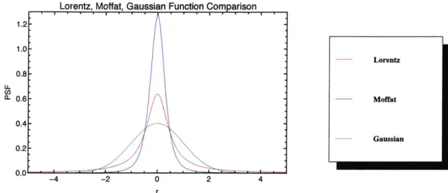
The figure below is a comparison of the three separate functions plotted together. It can be seen from this figure that the differences among each function come from the wings of the profile, the Lorentz and Moffat functions have more prominent and extended wings, and the Gaussian function has a more gradual dip into the wings. The wings of a star's PSF are what determine which model is a better fit.

14 12 10 8 6 4 2 0 2 8 10

1.2

U-CD

Lorentz, Moffat, Gaussian Function Comparison

1.0[ 0.8-0.6 0.4 0.2 0.0 -4 -2 0 2 4

Figure 4: Lorentz, Moffat, and Gaussian functions plotted together. Each function plotted is normalized to have an area of 1, and this plot shows the difference in the wings of each function which is ultimately what determines which model is a better fit for a star.

---_ Lorentz

--- Moffat

Methods

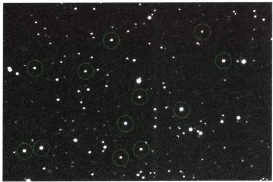
Five methods were chosen in order to calculate the centers of twelve stars on a test CCD frame. These methods included Circular Gaussian, Lorentzian, Moffat, Elliptical Gaussian, and center of mass fitting techniques. The figure below is an image of the star field used for analysis. The image was taken at Wallace Astrophysical Observatory on a 14" telescope with a SBIG STL-1001E imaging CCD camera with an exposure time of 60 seconds. The image scale was 1.2 arc sec/pixel.

Figure 5: Star field image taken at Wallace Astrophysical Observatory on a 14" telescope with a SBIG STL-1001E with an exposure time of 60 seconds and an image scale of 1.2 arc sec/pixel. The stars used for the PSF model comparison are circled.

For each fitting procedure, several parameters are fit to the data using a

least-squares fitting method of the specified function.

For the Circular Gaussian fitting method a Mathematica notebook was

used. The CCD image was read into the notebook, a star list was created

through a list of approximate coordinates for twelve stars on the CCD image

(accurate to one pixel), and then a for loop was created to run through the procedure for each star with varying box sizes. The procedure included

call-ing functions from a Mathematica package provided through the Planetary

Astronomy Lab in order to fit a gaussian curve to the star data. The

pa-rameters fit included the background, peak signal, x and y centers, diameter, and shape index. The fit was iterated through these parameters a maximum

of ten times, or until the calculated A were less than 10-. Once the selected

star had been fitted, the printed results included the calculated star

posi-tion.

A similar method was employed in order to fit a Lorentzian curve to the star data, where instead of the function psCircularGaussianStarMesh,

psCircularLorentzStarMesh was used. The same outputs were given for the

Lorentz fit including the calculated star positions and the chi-squared values.

The chi-squared value for the Lorentzian fit was approximately three times

greater than that of the Circular Gaussian fit, suggesting that the Circular

Gaussian model fit better to the data.

Twelve different box sizes (where box size would be double the size of an

30 pixels for the Mathematica notebook methods, and aperture sizes of 3 to 15 pixels were used for the IRAF methods. Varying box sizes were used to later determine which box size was best for comparing each method.

Within IRAF, the function used in order to calculate the center of each star was imexam. By editing rimexam, the aperture size and fitting method could be modified for each star. Imexam uses a nonlinear least squares fit profile of fixed center and zero background fit to the radius and flux val-ues of the background subtracted pixels to determine a peak intensity and full width at half maximum (FWHM) as described by the Science Software Group at STScI, (2000). The profile type can be chosen by the user as either Gaussian or Moffat. The profile equations are

I = Ic (e-( ) (fittype = "gaussian")

I = c (1 + (L)2)-0 (fittype = "moffat"),

where Ic is the peak value, r is the radius, and the parameters are -, a, and /.

The - and a values are converted to FWHM. Weights which are the inverse square of the pixel radius are used so that the contribution of the profile wings is reduced. The weight is wt = e-half-1 .2). A radially smoothed pro-file is produced by using an image interpolator function to fit to the region containing the object. Two FWHM measurements are computed using the enclosed flux radial profile. One is to fit a Gaussian or Moffat profile to the enclosed flux profile, and the Moffat # parameter may be fixed or included in the fit (for the fitting done in this paper the beta parameter was included in the fit). The second FWHM measurement directly measures the FWHM

independent of a profile model. This direct FWHM calculation is used for the iterative adjustment of the fitting radius.

A fifth method was also used, which involved the equation below for cal-culating the centroid of a star,

Xcenter, x (R[x, y] - B) E y (R[x, y] - B)

e E Ej (R[x, y] = - B) 'x

ZY

where R[x, y] is the pixel value at that point, and B is the local back-ground level, Chromey, Frederick R. (2010). The CCD image was read into a Mathematica notebook, and a function was created (see Appendix A) to calculate the centroid for a given star in the CCD image. In order to calcu-late the background value for each point, the mean of the top and bottom rows of the box were used. Though this method gave approximately the cor-rect location of the star, the results were heavily dependent on background values. If the value of the background was changed by only 1%, the cal-culated x and y coordinates differed by up to a few tenths of a pixel. For instance, when increasing the mean background value for the star located at

(370,145), the calculated x coordinate for the same box size changes from 369.703 to 369.295, a difference of 0.408. Given that the background value

is about 190, a 1% change would result in a background value of 191.9. The addition of a value of 2 to the background level should not cause such a large increase in the calculated coordinates, and so the model is too dependent on

background pixel values. The errors for the Lorentz and Circular Gaussian fitting notebooks were on the order of 0.01 pixels, and so an error of more than 0.1 pixel is unacceptable for determining the center of a star.

Aperture sizes between 3 and 15 pixels were chosen for both the Mof-fat and Gaussian fitting methods within IRAF. The coordinates were then placed into a list in Mathematica to determine the mean and then plot each coordinate's offset from the calculated mean. For instance, the offset graph of the x-coordinate of a star at approximate position (124, 301) is shown in

Figure 6. (124, 301) Magnitude 13.91 0.004 0.003-0.002 C> 5. 0.001 -0.000 0 -0.001 -0.002 -0.003 , . -4 6 8 10 12 14 Aperture (pixels)

Figure 6: x-coordinate offset from the mean of x-coordinates for varying aperture sizes. This plot was used in order to determine the best aperture size to use for model comparison, the least variation occurs for aperture sizes between 10 and 15 pixels and so an aperture size of 12 pixels is chosen.

It can be seen from the graph that there are large variations for aperture sizes of 3 through 6 pixels, however the offsets even out for offsets between 10

and 15 pixels. This suggests that an aperture size between 10 and 15 pixels would be best for comparing the results of each fitting method so that large variations in the data do not occur.

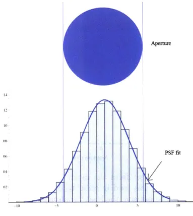
When choosing an aperture size, one wants to use an aperture that would allow for the greatest signal to noise ratio (SNR). If the aperture is too small, only part of the PSF will be detected. However, if the aperture is too large, more noise will be included due to the wings of the PSF, the background, and perhaps incident light from neighboring stars.

Aperhum 14: 10, PSF fit 04, 012

Figure 7: Illustration of amount of PSF detected for a given aperture size

To further refine the aperture choice, the flattened portion of the curve 20

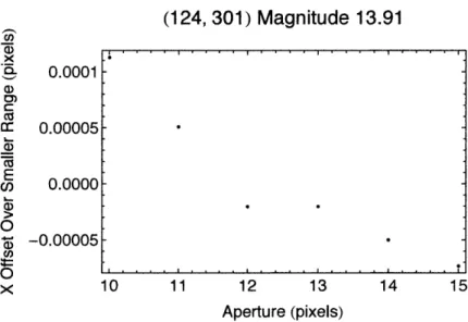
was examined to find for which aperture the least variation of the difference between the calculated center and the mean occurred. For example, the mean was calculated for the x offsets for apertures between 10 and 15 pixels and then the x offsets from this new mean were calculated for each aperture. The resulting plot for (124, 301) is below.

(124, 301) Magnitude 13.91 CD) CD C CU E CD) 0 0 0.0001 0.00005-0.0000 -0.00005 10 11 12 13 Aperture (pixels) 14 15

Figure 8: x-coordinate offset from the combined mean of x-coordinates for a smaller subset aperture sizes. The least variation occurs for aperture sizes of 12 and 13 pixels, and so an aperture size of 12 pixels was chosen for the model comparisons.

The section taken from the x offsets to scale with the full plot range of aperture sizes is below.

(124, 301) Magnitude 13.91 0.004 .X _0.003 0.002-Ca (D 0.001 -W 0.000 0 -0.001 CO) 4 -0.002 0 -0.00q3 9 10 11 12 13 14 15 Aperture (pixels)

Figure 9: x-coordinate offset from the combined mean of x-coordinates for a smaller subset aperture sizes scaled to the same y range as the full x-offset plot to show the lack of variation from the mean.

It can be seen from the plot above that the least variation from the mean exists for aperture sizes of 12 and 13 pixels. Several different stars of varying magnitudes were examined in the same way and the results for each star showed that the least variation occurred for aperture sizes of 12 or 13 pixels. Therefore, an aperture size of 12 pixels was chosen to compare the offsets of the star coordinates for each method. The FWHM for each star was found to be roughly 3 pixels, and aperture sizes chosen are typically 4-5 times the FWHM, Richmond (2006). So, an aperture size of 12-15 pixels would have been appropriate for comparing the residuals of each method.

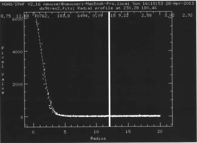
The enclosed flux can also be viewed from the radial profile, below is an image of the radial profile with a cut off at radius = _{12 pixels. At this radius,}

all of the main body of the star intensity is enclosed as well as some portion 22

of the wings.

Figure 10: Radial profile of a star with a cutoff at a 12 pixel radius. All of the fast-varying core of the star is included within this radius, along with a

Results

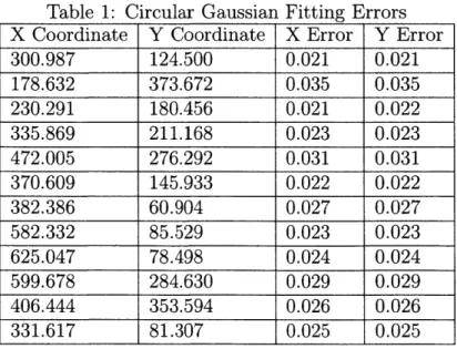
The tables below represent the calculated x and y coordinates and the error in fitting for each method. Errors are not available as an output for the IRAF package imexam. However, errors can be calculated for the IRAF package center which has an option to do the same Elliptical Gaussian fit as imexam, so these errors were used for the Elliptical Gaussian errors. Unfortunately, errors were not able to be produced for the Moffat fit because no IRAF package that uses a Moffat model produces error calculations.

Table 1: Circular Gaussian Fitting Errors X Coordinate Y Coordinate X Error Y Error

300.987 124.500 0.021 0.021 178.632 373.672 0.035 0.035 230.291 180.456 0.021 0.022 335.869 211.168 0.023 0.023 472.005 276.292 0.031 0.031 370.609 145.933 0.022 0.022 382.386 60.904 0.027 0.027 582.332 85.529 0.023 0.023 625.047 78.498 0.024 0.024 599.678 284.630 0.029 0.029 406.444 353.594 0.026 0.026 331.617 81.307 0.025 0.025 24

Table 2: Lorentz Fitting Errors

X Coordinate Y Coordinate X Error Y Error

300.946 124.495 0.068 0.068 178.614 373.640 0.088 0.088 230.296 180.480 0.070 0.070 335.867 211.162 0.071 0.071 472.009 276.276 0.075 0.075 370.615 145.939 0.068 0.068 382.394 60.965 0.073 0.073 582.330 85.550 0.064 0.064 625.049 78.508 0.063 0.063 599.705 284.622 0.070 0.070 406.457 353.554 0.071 0.071 331.627 81.271 0.071 0.071

Table 3: Elliptical Gaussian Fitting Errors X Coordinate Y Coordinate X Error Y Error

124.458 300.940 0.015 0.006 178.659 373.530 0.019 0.011 230.279 180.465 0.015 0.004 335.841 211.184 0.017 0.005 471.978 276.255 0.019 0.008 370.615 145.954 0.017 0.004 382.346 60.929 0.016 0.008 582.286 85.594 0.020 0.007 625.031 78.554 0.019 0.008 599.704 284.546 0.021 0.009 406.438 353.519 0.019 0.007 331.582 81.330 0.014 0.007

The mean of the x-coordinate offsets from the combined mean for each method were computed and are listed in the table below. The combined mean is the mean of the calculated centers for each method. For example, if the

center calculated at an aperture of 12 pixels for a Circular Gaussian fit was 180.456, for a Lorentzian fit was 180.48, for the IRAF Gaussian method was 180.465, and for the Moffat fitting method was 180.46, then the combined mean would be the average of each of these values. The table below shows that on average the Lorentz fit had the least variation from the calculated mean for each method, but that the variation between methods was very small.

Table 4: Average Difference from Combined Mean for Fitting Methods Coordinate Lorentz IRAF Moffat IRAF Gaussian

-0.0138 -0.0097 0.0126 0.0109

The mean x coordinate offsets from the combined mean for each method were computed and are listed in the table below.

Table 5: X Coordinate Offsets from Combined Mean for Fitting Methods X Coordinate Circular Gaussian Lorentz IRAF Moffat IRAF Gaussian

124 0.00107 -0.00352 0.001 0.001 178 -0.05943 -0.07741 0.068 0.068 230 0.00451 0.00965 -0.007 -0.007 335 0.01023 0.00852 -0.009 -0.009 472 -0.01852 -0.01403 0.016 0.016 370 -0.01470 -0.00866 0.016 0.006 382 -0.00890 -0.00144 0.005 0.005 582 -0.00813 -0.01044 0.009 0.009 599 -0.02494 0.00185 0.017 0.007 406 -0.01082 0.00216 0.005 0.005 331 -0.00871 0.00145 0.004 0.004 625 -0.02731 -0.02548 0.026 0.026

were computed and are listed in the table below.

Table 6: Y Coordinate Offsets from Combined Mean for Fitting Methods Y Coordinate Circular Gaussian Lorentz IRAF Moffat IRAF Gaussian

300 0.01396 -0.02733 0.006 0.006 373 0.04964 0.01659 -0.033 -0.033 180 -0.00775 0.01646 -0.004 -0.004 211 -0.00969 -0.01558 0.012 0.012 276 0.01553 -0.00063 -0.007 -0.007 145 0.00076 0.00633 -0.003 -0.003 61 -0.01350 0.04831 -0.017 -0.017 85 -0.00516 0.01502 -0.005 -0.005 284 0.00739 -0.00129 -0.003 -0.003 335 0.03686 -0.00311 -0.017 -0.017 81 0.01274 -0.02383 0.006 0.006 78 0.00661 0.01649 -0.012 -0.012

Analysis

The figures below represent the x and y coordinate offsets for each method. A legend that shows the magnitudes of each star is located on each plot.

0.20 0.15 0.10 0.05 0.00 -0.05 -0.10

Circular Gaussian X Coordinate Offsets

- , .v v 0 0 * * 0 0 * 0 S * :o 0 * . . . 6 8 10 12 14 4 * 13.91 * 15.87 + 12.88 A 14.78 * 15.57 0 13.89 o 13.50 0 14.21 A 15.36 V 14.95 * 14.93 . 15.24 Aperture (pixels)

Figure 11: Circular Gaussian x coordinate offsets for stars between 12.88 and 15.87 magnitude. Though outliers exist for stars of high magnitude and very small aperture sizes, there is a much smaller dispersion from the mean than for the Elliptical Gaussian and Moffat models, suggesting this model does not depend as much on aperture size.

U) X E 2 U-a) 0 0

0.6 0.4 E 0 LL 0.4 0.

Circular Gaussian Y Coordinate Offsets

-0

-

Figure 12: Circular Gaussian y coordinate offsets for stars between 12.88 and 15.87 magnitude. Though outliers exist for stars of low magnitude and very small aperture sizes, there is a much smaller dispersion from the mean than for the Elliptical Gaussian and Moffat models, suggesting this model does not depend as much on aperture size.

Lorentz X Coordinate Offsets SA A-- -A 8 10 Aperture (pixels)

Figure 13: Lorentz x coordinate offsets for stars between 12.88 and 15.87 magnitude. Though outliers exist for stars of low magnitude and very small aperture sizes, there is a much smaller dispersion from the mean than for the Elliptical Gaussian and Moffat models, suggesting this model does not depend as much on aperture size.

U-0 a, 0.10 0.05 0.00 -0.05 -0.10 * 13.91 w 15.87 * 12.88 A 14.78 15.57 13.89 0l 13.50 14.21 A 15.36 7 14.95 * 14.93 *15.24 4 6 12 14

Lorentz Y Coordinate Offsets ,0r '0 0 'U j

*

~ttt

S

Figure 14: Lorentz y coordinate offsets for stars between 12.88 and 15.87 magnitude. Though outliers exist for stars of low magnitude and very small aperture sizes, there is a much smaller dispersion from the mean than for the Elliptical Gaussian and Moffat models, suggesting this model does not depend as much on aperture size.

0.4 C 4) E 2 U-co 0 0.1 0.0

I

!

-IRAF Gaussian X Coordinate Offsets U +U -AI , , 1 . I V U -? . , . . . , , . . ,.U 8 10 Aperture (pixels) 12 14

Figure 15: Elliptical Gaussian x coordinate offsets for stars between 12.88 and 15.87 magnitude. The large spread from the mean over varying aperture sizes suggests that this model depends more on the aperture size than the

Lorentz or Circular Gaussian models

0. (D E 0 U-0 X 0.10 0.05 0.00 -0.05 -0.10 -0.15 * 13.91 . 15.87 *12.88 14.78 V 15.57 o 13.89 O13.50 o 14.21 A 15.36 * 14.95 * 14.93 m 15.24 4 6

IRAF Gaussian Y Coordinate Offsets - ... V S A 00 4 S S *0 8 10 Aperture (pixels) 12 V V 14

Figure 16: Elliptical Gaussian y coordinate offsets for stars between 12.88 and 15.87 magnitude. The large spread from the mean over varying aperture sizes suggests that this model depends more on the aperture size than the Lorentz or Circular Gaussian models

0.08 0.06 . CL E 0 0 A 0.04 0.02 0.00 -0.02 U 9 0 * 7 * S V 4 7 A U -0.04 -0.06 0 13.91 S 5.7 + 12.8 A 14.78 V 15.57 13.89 O13.50 -14.11 A 15.36 V 14.95 0 14.93 *15.24 4 6 A 0

Moffat X Coordinate Offsets

2 4 6 8 1

Aperture (pixels)

0 12 14

Figure 17: Moffat x coordinate offsets for stars between 12.88 and 15.87 magnitude. The large spread from the mean over varying aperture sizes suggests that this model depends more on the aperture size than the Lorentz or Circular Gaussian models.

0.1 a) a) 2 E 0 a) 0 0.0 0.0 -0.0 -0.1 0A 5.- A A A +- 0 -V V V 0 A+ll * * A 0 ! A V + A -5-e 5 - A-A A 0 Ua 0-" . * 13.91 *15.87 + 12.88 A 14.78 V15.57 13.89 o 13.50 S14.21 A 15.36 / 14.95 * 14.93 S15.24 0

Moffat Y Coordinate Offsets 0 A 0 A 9 0 0 a v * 9 9 9 o * . ~ 0 0 * U U U El A 0 A" . A 0 0 . " A-8 10 Aperture (pixels) 12 14

Figure 18: Moffat y coordinate offsets for stars between 12.88 and 15.87 magnitude. The large spread from the mean over varying aperture sizes suggests that this model depends more on the aperture size than the Lorentz or Circular Gaussian models.

0.08 El cl C E 0 2 U-0 0 . U 9 U 0.04 0.02 0.00 -0.02 -0.04 -0.06 4 0 0 A V A U . 13.91 * 15.87 + 12.88 A 14.78 V 15.57 13.89 o 13.50 ,1 14.21 A 15.36 14.95 0 14.93 S15.24 4 6 0.0j:.

Lorentz Y Coordinate Offsets A r% 4 6 8 10 12 14 Aperture (pixels) * 13.91 *15.87 *12.88 14.78 V15.57 13 ' 8 14.21 S15.36 14.95 * 14.93 a 15-14 LL

Circular Gaussian Y Coordinate Offsets

0.6 0.5 0.4-0.3 0.2 0.1 -0.0 -[ , * i I I I I I 2 4 6 8 10 12 14 Aperture (pixels)

Figure 19: y coordinate offsets for Lorentz and Gaussian models plotted to the same scale showing that there appears to be less deviation from the mean than when viewed from different scales. The IRAF models appear to have the greatest dispersion around the mean, but the Lorentz and Circular Gaussian models had the greatest outliers for small aperture sizes.

IRAF Gaussian Y Coordinate Offsets

4 6 8 10 Aperture (pixels) 12 14 * 5.87 A 14.78 V15.57 z13.50 14.21 A 15.36 V14.95 * 14.93 R 15.24 0.5-0.4' 0.3 E 0.2 0.1 >- 0.0 2

Moffat Y Coordinate Offsets

- I II I ! -I

4 6 8 10

Aperture (pixels)

12 14

20: y coordinate offsets for the IRAF Moffat and Elliptical Gaussian plotted to the same scale showing that there appears to be less de-from the mean than when viewed de-from different scales. The IRAF appear to have the greatest dispersion around the mean, but the z and Circular Gaussian models had the greatest outliers for small

aperture sizes. 0.5 0.4 CD 1 0.3 0.2 0.1 >- 0.0 . 0 2 0.5 0.4 $ 0.3-E 2 0.2- 0.1->- 0.0 2 Figure models viation models Lorent

I

~ , ~j

;

I

I

-0.20 0.15- 0.10-0.05 0.00 -0.05 -0.10 -0.152

Lorentz X Coordinate Offsets

4 6 8 10 12 14

Aperture (pixels)

IRAF Gaussian X Coordinate Offsets

E 2 IL 2 U-X * 13.91 * 15.87 - 12.88 A 4.78 53 13 2 3.91 1421 A 1..6 14.95 1493 15.24 * 13-91 *15.87 *12.U1 A14.71 V 15.57 13.19 :1 13.50 14-21 A15.36 14.95 * 1493 9 15.24 ca E 0 u-6 0.20 - 0.15- 0.10-0.05 0.00 -0.05 -0.10 -0.15 -0.20 0.15. 0.10, 0.05 0.00 U. -0.05 6 -0.10 -0.15

Circular Gaussian X Coordinate Offsets

4 6 8 10 12 14

Aperture (pixels)

Moffat X Coordinate Offsets

A f.4 V t 4 6 8 10 Aperture (pixels) 12 14

Figure 21: x coordinate offsets for the the four models plotted to the same scale showing that there appears to be less deviation from the mean than when viewed from different scales.

From the graphs above it can be seen that there is some stability for aperture sizes between approximately 10 and 13 pixels. Also, the largest outliers occur for stars of high magnitude and for fits with small aperture sizes. This is to be expected because if the aperture size is too small the flux enclosed is not complete, and for high magnitude stars it is more difficult to fit a PSF because of the low SNR. It can also be determined that there is a much smaller spread from the mean for the Lorentz and Circular Gaussian offsets than for the Elliptical Gaussian and Moffat offsets. This may indicate that

A 0.20 0.15. 0.10 0.05 0.00 -0.05 -0.10 * -0.15 2 4 6 8 10 12 14 Aperture (pixels) * .. 0 0 * * * * * * S S 2 2 * 15.87 + 12.U A 14.789 V 1537 =13.50 341 A 15.36 . 14.95 01493 3 5-24 * 13.9: * 5.9'. * 12.1 A 147 V 15.5'. 13.8 213.5( 14.2: 15.3( 14.9 * 14.9 - l5s2

the Lorentz and Circular Gaussian models are less dependent on aperture size than the Moffat and Elliptical Gaussian models.

The magnitudes of each star were calculated via imexam within IRAF. The average magnitude for each star was used when determining whether or not a magnitude effect existed in the data results.

0.06_ 0.04 - Lorentz Cd 0.02 -0 Circular Gaussian 0.00 -( Moffat E -0.02-02 -0.04 ' Elliptical Gaussian -0.06--0.08 - , . , , , , .., , ., , ,. , , , , , , , , ,__ _,_,_,_ _ 13.0 13.5 14.0 14.5 15.0 15.5 Magnitude

Figure 22: x-coordinate offsets for stars of varying magnitudes calculated from the combined mean of each method. It can be seen that a magnitude effect exists, especially for very high magnitudes with a difference of 0.06 pixels for a magnitude of 15.87, but that it is only apparent for magnitudes greater than 15.

It can be seen from the plot above that some magnitude effect exists for stars between magnitudes of 12.88 and 15.87, however the effect appears small except for magnitudes greater than 15. The largest offset from the combined mean is about 0.06, but for most magnitudes the offset is between 0.02 and 0.04, which is within the fitting error. For increasing magnitudes,

the offsets for each fitting method have a greater dispersion around 0 and also have a greater dispersion from each other. However, the Mathematica fitting techniques (Circular Gaussian and Lorentz) stay close to one another. The same is true for the IRAF fitting techniques (Moffat and Gaussian). This tracking may be a result of the accuracy and precision of each fitting method.

Circular Gaussian Vector Plot 400 350 -\ 300N 150 100 1-0 x pixchs 350 300 250

IL

Lorentz Vector Plot

100 200 300 400

x pixels

TRAF Moffat Vector Plot

A.-a--100 200 300 400 500 600 x Pixels 350 300 250 M5 >%200 150 100 50

TRAF Gaussian Vector Plot

- -' I -N\ . .i d .. .. . . . . 100 200 30D 400 x pixels SW 600

Figure 23: Vector representation of x and y residual offsets for each method scaled by 10. It appears that each method has some dependence on position on the CCD chip which most likely has to do with each star's orientation on the optical axis.

* - I :1' / - ----l i' 500 60D 350 300 250 ~'200 150 1 100 50 0 0 -r." 0

The four plots above show a vector representation of the x and y residual offsets for each method. The mean of each method was calculated for the position of each star at an aperture of 12 pixels and the offsets represent the method's difference from this calculated mean. The offsets are scaled

by a factor of 10 to more easily represent the vectors. It appears that the

Circular Gaussian and Lorentz methods from the Mathematica notebook are inverted in their dependence on CCD chip position compared to the Moffat and Elliptical Gaussian fitting methods. The large offsets on certain positions on the chip could result from a magnitude effect or a star's alignment on the optical axis. The largest variation between the two vector offsets is a value of 0.0333329 pixels. So, if accuracy beyond that value is needed for certain astrometry calculations, more care has to be taken in choosing the PSF model.

The figures below show this effect by placing darker spots where there are stars of higher magnitude. It appears that the Lorentzian model is unaffected

by the higher magnitude stars in the upper right hand corner of the star field.

This may indicate that for some high magnitude stars the Lorentz model is better at fitting a PSF.

mussian Vector , , , , ,7, 400 rI 3350 300 250 2100 150 100 so -11i 00 -1 \ I

4.

Moffat Veclor ilA

100 200 300 400 x pixels 500 00 30 2300 0 200 ISO 200 so r1aus 32011 Vector Plot ~I \ \ \ \ \ \ \ \ 100 2(10 3W0 Ox)

Figure 24: Magnitude effect on vectors of residual offsets for each method. Brighter stars are represented by yellow, darker stars by green with 12.88 as the lowest magnitude and 15.87 as the highest magnitude.

330 300 250 1l 200 150 200 100 200 Low Magniftde 400 330 300 250 ~200 (00) s0 High Magmtude !Vector Plot 40D r I, , 400

Conclusion

From the comparisons shown in this paper, it appears that there is very little variation among each fitting method used in order to determine the centers for stars of varying magnitudes. The fitting method that produced the smallest errors in fitting was the Elliptical Gaussian method from IRAF's imexam package (errors ranged on the order of 0.01-0.02 pixels). The Lorentz fitting method had the largest errors when fitting and appeared to be the worst model for the data set provided (errors were on average 0.07 pixels).

The errors for the Circular Gaussian were also small (on average 0.02 pixels), and so it seems that a Gaussian PSF fit would be best for determining the centers of isolated stars for magnitudes between 12.88 and 15.87. It was also determined that the center of mass method for calculating a star centroid was inadequate and too dependent on sky background calculations. However, there also seemed to be a model dependence on position on the CCD chip. Therefore, if accuracy greater than 0.033 pixels is necessary for performing astrometry, more steps need to be taken in order to determine which model will best fit the star.

Future work for this endeavor would include comparing the results from the test CCD image to an extensively studied image so as to have a more clear idea of the true center of a star. In order to have a better idea of the true center of a star, one would have to work indirectly from parallax or proper motions of stars and choose the model that most accurately describes the

kinematics. However, only one frame is provided in this study and so that avenue was not possible. Therefore, for future work on this topic multiple frames taken over a series of months should be studied so that the true center of the star can be indirectly determined for comparison.

References

[1] Trujillo,I., Aguerri, J.A.L,Cepa, J. Gutierrez, C.M.2001,328,977

[2] Weisstein, Eric W. "Lorentzian Function." From MathWorld-A Wolfram Web Resource. http://mathworld.wolfram.com/LorentzianFunction.html

[3] "Imexamine." Imexamine. Science Software Group at STScI, 3 Sept. 2000. Web. 07 May 2013.

[4] Chromey, Frederick R. "Digital Images from Arrays." To Measure the Sky: An Introduction to Observational Astronomy. Cambridge: Cambridge UP, 2010. 299-300. Print.

[5] Noel, E.D. Noelia, Gallart, Carme, Costa, Edgardo, Mendez, Rene A "Old Main-Sequence Turnoff Photometry in the Small Magellanic Cloud. I. Constraints on the STar Formation History in Different Fields,2006

[6] Richmond, Michael. "Simple Aperture Photometry by Hand." Simple Aperture Photometry by Hand. N.p., 12 Apr. 2006. Web. 09 May 2013.

Appendix A

XCenter[subframe_ , x_, y_, xstart_, rend , ystart_, yend] :=

Sum[

Bum[

x *

(subframe [ [y, x]]

-((Sus(data ( [yatart, x]], x, xstart, xend)] (xend - xstart) +

(Sum [data [ [yend, x]], {x, xstart, xend}] I (xend - xstart))) 12) ,

(x, _xstart, xend)], {y, ystart, yend)]

(Sum[ sum[

(subframe[ [y, x]]

-((Sum(data [ [ystart, x], (x, xstart, xend)/ (xend - xstart)) + (Sum[data [ [yend, x], (x, xstart, xend)] / (xend -ratart))) /2),

(x, xstart, xend)], fy, ystart, yend)])

TCenter[subframo, x_, y_, xatart_, rend_, ystart , yend_]

Sum[

Sum[

y*

(subframe [ [y, x]]

-((Sum (data [ [ystart, x]], (x, xstart, xend)]1 (xend - xsatart)) +

(Sum [data [[ yend, x]], (x, xstart, xend)] / (xend - xstart) /2),

(x, xstart, xend)], fy, ystart, yend)]!

(SuM[l

sum

(subframe[[y, x]]

-((Sum[data ( [yatart, x]], {x, xstart, xend)]/ (xend - xsatart) + (Sum[data [ [yend, x]], ( x, xstart, xend)]! (xend -xstart))) /2) ,

(x, xsatart, xend)], (y, ystart, yend)])

Figure 25: Mathematica functions written to calculate dinates for a star from a CCD frame

X and Y center

coor-Appendix B

The figures below represent offsets from the mean for calculated centers at aperture sizes ranging from 3 to 15 pixels for the x and y coordinates of each method.

-j

Circular Gaussian X-Coordinate Offsets

(124, 301) Magnitude 13.91 0.004- 0.003- 0.0020.001 - 0.000- -0.001- -0.002--0.003. 4 6 8 10 12 14 Aperture (335, 211) Ma nitude 14.78 0.005 . .. 0.000- -0,005- -0.010- -0.015--0.020,, 4 6 8 10 12 14 Aperture (382, 61) Magnitude 15.24 0.00 - -0.02- -0.04- -0.06-4 6 8 10 12 14 Aperture 0.0 0.0 0.0 -0.0 -0.0 -0.0 -0.0 1 (178, 373) Magnitude 15.87 0.005-5 0.000 . -0.005. < -0.010 -0.015 .. .. . . . . 4 6 8 10 12 14 Aperture ru 'P) (472, 276) Magnitude 15.57 0.04 -- ...' ..'.. '.. . 0.03-0.02. 0.01 - 0.00--0.01 4 6 8 10 12 14 Aperture (582,85) Magnitude 13.5 0.02 . 0.00- -0.02- -0.04- -0.06- -0.08- -0.10-(599, 284) Magnitude 15.36 .4 2 -0. 2 4 6 4 6 8 10 12 14 Aperture a, x6 0.0 0.0 -0.0 -0.0 -0.0 -0.0 4 6 8 10 12 14 Aperture (406, 353) Magnitude 14.95 0- 1- 2-3. A '- ' 4 6 8 10 12 14 Aperture (230, 180) Magnitude 12.88 0.000--0.005 -0.010 4 6 8 10 12 14 Aperture (370, 145) Magnitude 13.89 0.02 0.00. 9 -0.02-x -0.04 -0.06. 4 6 8 10 12 14 Aperture (625, 78) Magnitude 14.21 0.020, 0.015 0.010 5 0,005, < 0.000- -0.005--0.010 1 -.,.,. 4 6 8 10 12 14 Aperture (331, 81) Magnitude 14.93 0.20. 0.15- 0.10-x 0.05 0.00 -0.05-4 6 8 10 12 14 Aperture 1a, U, -U, I

A4

Circular Gaussian Y-Coordinate Offsets

(124, 300) Magnitude 13.91 0.06 - 0.04- 0.02- 0.00--0.02 --0.04. 4 6 8 10 12 14 Aperture (335, 211) Magnitude 14.78 0.025 - ' 0.020. 0.015-0.010 0.005-4 6 8 10 12 14 Aperture 0) (382, 61) Magnitude 15.24 -84.98 ' -84.99 -85.00 .z -85.01 5 -85.02 -85.03 F. ,... , .. . T ... 4 6 8 10 12 14 Aperture (406,353) Magnitude 14.95 0.005-0.000. -0.005 -0.010- --0.015. -0.020- -0.025-4 6 8 10 12 14' Aperture (178, 373) Magnitude 15.87 0.01 0.00 - -0.01- -0.02- -0.03--0,041, 4 6 8 10 12 14 Aperture (472, 276) Magnitude 15.57 0.005-0.000. S -0.005- 0 -0.010 - -0.015-4 6 8 10 12 14 Aperture (582, 85) Magnitude 13.5 0.020 b 0.015 0.010. 0.005 . 0.000 --0.005 ... , 4 6 8 10 12 14 Aperture (331,81) Magnitude 14.93 4 6 8 10 12 14 Aperture 0.6 0.4 0.2 0.0 a, .5 (230, 180) Magnitude 12.88 0.02- 0.01-0.00 -0.01 4 6 8 10 12 14 Aperture (370, 145) Magnitude 13.89 0.010 0.005 0.000 -0 .0 0 5 ... 4 6 8 10 12 14 Aperture (599, 284) Magnitude 15.36 0.002. 0.000. -0.002--0.004. -0.006 -0.008 -0.010, . 4 6 8 10 12 14 Aperture (624,78) Magnitude 14.21 0.010 0.005 0.000 4 6 8 10 Aperture 12 14 a, cfl S 0

-9

Lorentz X-Coordinate Offsets

(124,301) Magnitude 13.91 0.006 0.004-0.002 0.000 0.002 - e * . . 4 6 8 10 12 14 Aperture (335,211) Magnitude 14.78 0.02. 0.01. 0.00--0.01 -0.02--0 .0 3 :-= ... ,... .... , ... , .... . 4 6 8 10 12 14 Aperture 0.02 0.00 -0.02 ' -0.04 -n nR (382,61) Magnitude 15.24 75 0 x 02 x 4 6 8 10 12 14 Aperture (599,284) Magnitude 15.36 0.02. . 0.00--0.02 -0.04= = -0.06 - X -0.08 4 6 8 10 12 14 Aperture (178,373) Magnitude 15.87 0.006 ' 0.000 -0.002---0.004 . -0.006 4 6 8 10 12 14 Aperture (472, 276) Magnitude 15.57 0.020= 0.015 0.010 Ln 0.005' E 0.000 =* x -0.005 . -0.0,10, 4 6 8 10 12 14 Aperture 0.02 0.00 -0.02 -0.04 -0.06 -0.08 0.01 0.0 -0.01 -0.0 -0.0 -0.0 (582,85) Magnitude 13.50 4 6 8 10 12 14 Aperture (406,353) Magnitude 14.95 3= 4 6 8 10 12 14 Aperture 02 'C En 6 'C (230,180) Magnitude 12.88 0.010- 0.005-0.000. -0.005--0.010 . -0.015 -0.020--0.025 E. . . . . .. . . . 4 6 8 10 12 14 Aperture 0.02 0.01 0.00 -0.01 -0.02 -0.03 -0.04 -0.05 0.015 0.010 0.005 0=000 -0.005 -0.010 0.10 0.08 0.06 0.04 0.02 0.00 -0.02 (370,145) Magnitude 13.89 4 6 8 10 12 14 Aperture (625,78) Magnitude 14.21 4 6 8 10 12 14 Aperture (331,81) Magnitude 14.93 4 6 8 10 12 14 Aperture 0, a, x 02 x ' ' ' '

Lorentz Y-coordinate Offsets (178,373) Magnitude 15.87 0.02-0.01 -0.00. -0.01 - -0.02- -0.03--0.04,-, 4 6 8 10 12 14 Aperture 0.02C 0.015 0.01 0.005 0,00C -0.005 -0.010 0.015 0.010 0.005 0.000 -0.005 -0.010 0.03 - 0.02-0.01 " 0.00. -0.01 -0.02- -0.03-(472,276) Magnitude 15.57 -4 6 8 10 12 14 Aperture (582,85) Magnitude 13.50 4 6 8 10 12 14 (230,180) Magnitude 12.88 0.03 ... .. 0.02. * 0.01-2 0.00. 0 0.01 --0.02 . - 0 .0 3 ,,, , ... 4 6 8 10 12 14 Aperture (370,145) Magnitude 13.89 0.015 - . -0.010. 0,005-01000,-'. -0.005 -0.010-4 6 8 10 12 14 Aperture a, (j 0.010 0.005 0.000 -0.005 Aperture (406,353) Magnitude 14.95 4 6 8 10 12 14 Aperture 0.4 0.3 0.2 0.1 0.0 (373,78) Magnitude 15.87 .. .... ....... .. 4 6 8 10 12 14 Aperture (331,81) Magnitude 14.93 4 6 8 10 12 14 Aperture (335,211) Magnitude 14.78 0.020 0.015-3 0.010 n 0.005-9 0.00 >- -0.005- -0.010--0.015 4 6 8 10 12 14 Aperture 0.010 0.005 0.000 -0.005 >- -0.010 -0.015 -0.020 (382,61) Magnitude 15.21 -. 4 6 8 10 12 14 Aperture (599,284) Magnitude 15.36 0.006-0.004. 0.002 -0.000 -0.002 -0.004 - 7 4 6 8 10 12 14 Aperture (382,61) Magnitude 15.24 a, 0.010 0.005 0.000 -0.005 -0.010 -0.015 -0.020 4 6 8 10 12 14 Aperture 0 w 0 0

-j

Moffat X-Coordinate Offsets

(124, 301) Magnitude 13.91 0.02...-...r '' -0.01, 0.00. -0.01 --0.02 -0.03 -. , , , , , 4 6 8 10 12 14 Aperture (335,211) Magnitude 14.78 0.04,- 0.02.- 0.00--0.02 -0.04- . -4 6 8 10 12 14 Aperture x U' 'C (582,85) Magnitude 13.50 0.00--0.05 x x -0.10-4 6 8 10 12 14 Aperture (178,373) Magnitude 15.87 0.10.. 0.05-0.00. -0.05--0.10 , 4 6 8 10 12 14 Aperture (472, 276) Magnitude 15.57 0.02-0.00' -0.02--0.04 ... 4 6 8 10 12 14 Aperture (625,78) Magnitude 14.21 0.06 ' 0.04- 0.02- 0.00- -0.02- -0.04--0.06L 4 6 8 10 12 14 Aperture (230,180) Magnitude 12.88 0.05 D 0.00- -0.05- -0.10-2 4 6 8 10 12 14 Aperture U' x U' x (370,145) Magnitude 13.89 0.02. 0.01 -0.00; -0.01 --0.03 -0.04,, 4 6 8 10 12 14 Aperture (599,284) Magnitude 15.36 0 .0 8 . . 1 -1 .......- .-- 0.06, 0.04- 0.02-0.00? -0.02. -0.04--0,06F 4 6 8 10 12 14 Aperture 406,353) Magnitude 14.95 4 6 8 10 12 14 Aperture (331,81) 0.04, 0.02-S0.00 xC -0.02-. -0.04 Magnitude 14.9 4 6 8 10 12 Aperture 14 3 (382,61) Magnitude 15.24 0.05 0.00 -0.05 _' -0.10 4 6 8 10 12 14 Aperture V' 'C U' 0.04 0.02 0.00 -0.02 -0.04 -0.06 -0.08

Moffat Y-Coordinate Offsets (124,301) Magnitude 13.91 0.02. . W 0.00 o -0.021 > -0.04. -0.06 4 6 8 10 12 14 Aperture (335,211) Magnitude 14.78 0,02-0.00 - -0.02--0.04. -0.06L 4 6 8 10 12 14 Aperture (582,85) Magnitude 13.50 0.06- 0.04-0.02. 0.00--0.02. -0.04 L .. 4 6 8 10 12 14 Aperture (406,353) Magnitude 14.95 0.01 . 0.00 . . . --0.01 --0.02,_ 4 6 8 10 12 14 Aperture (178,373) Magnitude 15.87 0.02-En 0.00' -0.02- -0.04-4 6 8 10 12 14 Aperture CD (472,276) Magnitude 15.57 0.06: 0,04 -0.02 0.00.6 -0.02 - -0.04--0.06 4 6 8 10 12 14 Aperture (624,78) Magnitude 14.21 0.04. 0.02 . 0.00~ -0.02-4 6 8 10 12 14 Aperture (331,81) Magnitude 14.93 0.06 F-0.04. 0.02 -0,00. -0.02 -0,04 -4 6 8 10 12 14 Aperture (230,180) Magnitude 12.88 0.02 0.01 0.00 -0.01 4 6 8 10 12 14 Aperture (370,145) Magnitude 13.89 0.04 0.03. 0.02. 0.01 0.00. -0.01. -0.02 ,.., ,.., .. 4 6 8 10 12 14 Aperture (599,284) Magnitude 15.36 0.02 0.00 -0.02 -0.04 4 6 8 10 12 14 Aperture (382,61) Magnitude 15.24 0.08 0.06 0.04-0.02 0.00. -0.02 . - - - - - . -0.04 - ---4 6 8 10 12 14 Aperture Cd' a' Cd' ---q