Comparing complex networks: in defence of the simple

PAPER • OPEN ACCESS

Comparing complex networks: in defence of the simple

To cite this article: Johann H Martínez and Mario Chavez 2019 New J. Phys. 21 013033

View the article online for updates and enhancements.

PAPER

Comparing complex networks: in defence of the simple

Johann H Martínez and Mario Chavez

INSERM-U1127, CNRS UMR7225, Sorbonne Université, ICM-Hôpital Pitié Salpêtrière, Paris, France E-mail:johemart@gmail.com

Keywords: network distances, complex systems, dissimilarity, kernel distance

Abstract

To improve our understanding of connected systems, different tools derived from statistics, signal

processing, information theory and statistical physics have been developed in the last decade. Here, we

will focus on the graph comparison problem. Although different estimates exist to quantify how

different two networks are, an appropriate metric has not been proposed. Within this framework we

compare the performances of two networks distances

(a topological descriptor and a kernel-based

approach as representative methods of the main classes considered) with the simple Euclidean metric.

We study the performance of metrics as the efficiency of distinguish two network’s groups and the

computing time. We evaluate these methods on synthetic and real-world networks

(brain

connectomes and social networks), and we show that the Euclidean distance efficiently captures

networks differences in comparison to other proposals. We conclude that the operational use of

complicated methods can be justified only by showing that they outperform well-understood

traditional statistics, such as Euclidean metrics.

1. Introduction

Despite the success of complex networks modeling and analysis, some methodological challenges are still to be tackled to describe and compare different interconnected systems. Identifying and quantifying dissimilarities among networks is a challenging problem of practical importance in manyfields of science. Given two graphs

¢

{G G, }, we aim atfinding an injective and real-valued function h that mapsG ´ G¢  "{G G, ¢}. Functionsh G G( , ¢)that quantify the(dis)similarity between two networks have been been studied in several areas such as chemistry, protein structures, social networks up to neuroscience, among others[1–4]. Without an

h uniqueness, different approaches have been proposed including graph edit operations, distances based on divergences, spectral parameters, kernels, or different combinations of the previous[5–11].

Although several of these dissimilarity metrics have been developed in the framework of complex networks and can capture the connectivity structure at different different levels(degrees, walks, paths, etc), the natural question arises as to whether a simple measure(e.g. the Euclidean distance) is able to quantify and distinguish two networks.

In this work, we consider three classes of the function h: thefirst class, which represents a large bunch in the literature, quantifies local changes via structural differences. These metrics may range from the simplest Euclidean distance[12–14] to more elaborated algorithms that assign costs of different operations to map

nodes/edges of G to theirG¢counterparts[5,15,16]. Another distance class considers topological descriptors

that map each graph into a feature vector(e.g. degree distribution, nodes centrality, etc). These vectors are compared with any multivariate statistical distance or information-type metrics to compute the

graph dissimilarity[10,17,18]. We notice that considering one type of feature may imply to lose topological

information from others parameters, and the price of a complet caracterisation may be paid with more runtime. The last class considered here includes kernel-based approaches that compare global substructures(i.e. walks, paths, etc). These methods capture global information of networks (e.g. the graph Laplacian) considered in a metric space, where a defined inner product directly estimates its dissimilarity [19]. Kernel-based methods, OPEN ACCESS

RECEIVED 22 October 2018 REVISED 2 January 2019 ACCEPTED FOR PUBLICATION 21 January 2019 PUBLISHED 31 January 2019

Original content from this work may be used under the terms of theCreative Commons Attribution 3.0 licence.

Any further distribution of this work must maintain attribution to the author(s) and the title of the work, journal citation and DOI.

however, often integrate over local neighborhoods, which renders these approaches less sensitive to small or local perturbations[7].

In our study we show than the use of a simple Euclidean metric may provides good performances to asses graph differences, when compared to other more complicated functions. We propose a framework for measuring the performance of functions hʼs applied on undirected-binary graphs of equal sizes. We define the hʼs performance in terms of ‘discriminability’ and ‘runtime’. The former is the capability of h for discriminating two sets of networks associated to two different groups. The latter is simply the computing time.

2. Comparing network distances in synthetic and real networks

In what follows, we compare the performance of the standard Euclidean distance(Df), the dissimilarity measure

(Dd) defined in [10], and the graph diffusion kernel distance (Dk) [9], from each of the classes mentioned above.

As each class encompasses many metrics with a common core(e.g. Frobenius norm, Information theory,

Kernel-based types), we chose one of the recent published distances for each class to compare them. For these algorithms, we evaluate the discriminability and runtime in different synthetic and real-world networks. We show that the Euclidean distance substantially outperforms other methods to capture differences between networks of the same size.

2.1. Euclidean distance

Assuming that{A1, A2} are the adjacency matrix representations of graphs {G1, G2}, we have the Euclidean

distance defined by:

= -  ( )

Df A1 A2 F, 1

where  · Fdenotes the Frobenius norm.

2.2. Network structural dissimilarity

This dissimilarity measure captures several topological descriptors[10]: network distance distributions m{A A1, 2},

node-distance distribution functionsNND{A A1, 2}(local connectivity of each node), α-centrality distributions

a{ }

P A A1, 2 , the equivalent for their graph complementsPa{A Ac, c}

1 2 and several tuning parameters a{ ,w w w1, 2, 3}.

The network distance is obtained via the Jensen–Shannon divergence Γ between different feature vectors.

m m = G + -+ ⎛ G a a + G a a ⎝ ⎜⎜ ⎞_⎠⎟⎟ ( ) ∣ ( ) ( ) ∣ ( ) ( ) ( ) D w w A A w P P P P , log2 NND NND 2 , log2 , log2 . 2 A A A A A A d 1 2 1 2 3 c c 1 2 1 2 1 2 2.3. Kernel-based distance

A recently proposed distance is based on diffusion kernels[9]. This method estimates the differences between

diffusion patterns of two networks undergoing a continuous node-thermal diffusion. A set of distances at different scales t can be obtained by means of the Laplacian exponential kernels_e-t{A A1, 2}. The kernel-based

distance is obtained by[9]:

 

= { (- )- (- ) } ( )

Dk max exp t exp t , 3

t 1 2 F

where idenotes the graph Laplacian of network i.

To assess the performances of these functions to capture network’s differences, we consider a network A and a set of perturbed networks{Ap} generated with a random rewiring (with probability p) of original network A.

We evaluate hʼs by computing the differences between perturbed versions {Ap} and its original configuration A.

For low values of p, networks are very similar. Network differences are expected to increase with p. The aim of this random rewiring is to simply produce a random perturbation similar to that used when studying the network robustness[20]. We then evaluate the dissimilarity value after a given fraction of links is rewired while

preserving the number of links and connectedness. 2.4. Benchmark tests

We build binary Barabasi–Albert (BA), Strogatz–Watts (SW) [20] and Lancichinetti–Fortunato–Radicchi (LFR)

[21] models with L links and N=100. In the BA model, the mean degree is set to 4 and the exponent of the

degree distribution is, by construction, 3. For SW model, the number of initial neighbors is K=4 for a

= *

L N K edges and mean degree equal to2K. In LFR model, the mean and maximum degree is set to 15 2

and 30, respectively. LFR model consists of 100 nodes splitted in 5 modules of{30, 24, 16, 16, 14} nodes each, and 635 links. Degree and community distribution exponents are 3 and 2 with a mixing parameter of 0.2. For each model we recreate a continuous perturbation process by reshuffling their links with and incremental rewiring probability step p=0.001. This allows us to create a set of∣∣{Ap}∣∣=1000connected networks, each of them withL*prewired links.

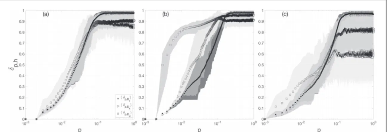
Letδp,hbe the network-distance vector that contains all differences between perturbed networks{Ap} and A

measured for a given metric h. We compute the averaged profilesádp h,ñas well as the 5th–95th percentiles (figure1). As expected, all the averaged profiles display monotonically increasing curves that reach out certain

saturation around p= 10−1. Results suggest that all the measures(including the Euclidean distance) are sensitive to small structural changes(10% of reshuffled links), and reflect well the structural perturbations. Beyond this threshold(p > 10−1), however, all functions cannot distinguish between a graph A and its perturbed version {Ap}. Results also show that, despite the non-trivial heterogeneous connectivity of the LFR model, the

network-distance profiles are quite similar. Further, results clearly indicate that Euclidean network-distances has lower variability than the other two distances.

2.5. Assessment of performances

Our results suggest that the dissimilarity curve obtained by comparing a given network and its different perturbed versions captures relevant features of the original connectivity, which suggests it can be directly used to compare two networks. To assess the different metrics’ performances we quantify the ‘discriminability’ and the‘runtime’. Discriminability assesses whether a given function h is sensitive at certain perturbation p, and whether it is suitable to distinguish two different group of networks at a given p. Discriminability is defined as the percentage of times a function h distinguishes the differences of each group of networks at certain perturbation level. The more times h distinguishes two different datasets, the better the h discriminability is. In addition, runtime simply measures the h execution time. The faster a given function h estimates the differences, the better the corresponding metric is. For the sake of applicability we tested the performance of different hʼs in real networks.

2.6. Real networks

In this work, we evaluate metric’s performances upon two dataset of different nature: functional brain connectomes and social networks. We use a recently published brain connectivity dataset[22], which includes

functional connectivity matrices estimated from magnetoencephalographic(MEG) signals recorded from 23

Alzheimer patients(P) and a set of controls subjects (C) during a condition of resting-state with eyes-closed [23].

Alzheimer disease is caracterised by anatomical brain deteriorations, which are reflected in an abnormal brain connectivity. MEG activity was reconstructed on the cortical surface by using a source imaging technique[23].

Connectivity matrices were obtained from N=148 regions of interest by means of the spectral coherence between activities in the band of 11–13 Hz. We specifically focused on the functional connectivity in this frequency band, which is particularly activated during resting activity with closed eyes, and it reflects the main functional connectivity changes accompanying the disease[24]. All the recording parameters and

pre-processing details of connectivity matrices are explained in[23].

Following the procedure of[25], we thresholded each connectivity matrix by recovering its minimum

spanning tree and thenfilling the network up with the strongest links until to reach a mean degree of three. Our

Figure 1. Network-distances as a function of the rewiring probability p. For visualization purposes, each profile was normalized by dividingδp,hby the maximum value obtained over the whole range of perturbations. All symbols represent the averages over 100 realizations, and shaded areas indicate theirs 5th and 95th percentiles.(a) For the BA networks, (b) for the SW model and (c) for the LFR benchmark. In both models,ádp h,ñvalues were estimated for the same rewiring probability.

criterion admits that the weighted links of the raw networks had been previously validated, either maintained or canceled[26]. This thresholding criterion ensures a trade-off between network efficiencies (both global and

local) and wiring cost. In [25,26], theoretical and numerical results show that, for a large class of brain networks

(including functional ones as those used in our study), this balance is obtained when the connection density ρ follows a fractal scaling regardless of the network size according to the power-lawρ = 3/N. The resulting connectivity networks are binary adjacency matrices with N= 148 nodes with L = 222 links.

A direct comparison of connectivity matrices between the graphs of two groupsA Î{PC does not not} allow to distinguish them. This result agrees with previous studies that found group differences related to very local changes in connectivity[23,24]. Authors in [23] for instance, found that only 3% and 4% of the nodes

accounts for the connectivity differences between groups, when different frequency bands are combined in the analysis.

The approach proposed to detect global network differences between those groups is based on the dissimilarity curve of each network. For this, each connectivity graph A isfirstly perturbed by randomly choosing l links "l = 1, 2,¼,Land reshuffling them such that the graph remains connected. We get thus a

set of∣∣{ }∣∣Al =222perturbed networks. We then compute the network differences between all pairs(A, Al).

Wefinally repeat this procedure for 20 independent realizations. The distances profiled_{l h}s

, results from the

average of the network differences across realizations for a given subject S. The set of∣∣{dl hs,}∣∣=23distances profiles per group (one for each subject) is used to compare the differences captured by h when l links are rewired. A function h distinguishes two populations d{ _{l h}s_,}P {d_{l h}s_,}Cat certain level l, if the group differences are statistically different at that perturbation level. Discriminability is defined as the hits percentage along all L perturbations, i.e. the number of times the null hypothesis Hoof no difference between the two groups is

rejected. To assess significant differences, we used a non parametric permutation test allowing 500 permutations for each l and we reject Hoat p„0.05 (corrected by a Bonferroni method).

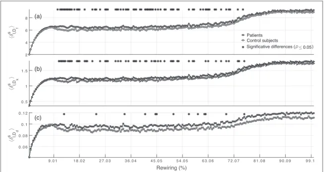
The mean distance profilesád_{l h}s ñ

, for each h are plotted infigure2. As in synthetic models, profiles show a

monotonically increasing behavior. At low rewiring percentages(„11%) there is no significant differences at group level. For small perturbation levels, functions h cannot distinguish connectivity between groups. Something similar is observed when links perturbation are above≈70%. On the other hand, Dfappears as the

one with the highest discriminability closely followed by Dk, while Ddappears with lowest one. Results clearly

suggest that Euclidean distance distinguishes better the two groups of networks considered here.

We now move our attention to the comparison of social networks. We applied our approach to the analysis of connectivity differences between two social networks. Each connectivity matrix contains the friendship and socioemotional interactions among workers in a tailor shop in Zambia, during two periods of time(seven months apart), immediately before and unsuccessful (t1) and a successful (t2) strike, respectively [27]. Networks

Figure 2. Mean distances pro_{files d}á l hs,ñfor P(black) and C (white) are plotted as a function of the rewired l links (rewiring %). The existence of group statistical differences in each rewiring step are highlighted at the top of each panel by the black stars.(a) Euclidean distance yields a discriminability of 32.89%.(b) The kernel-based distance yields a discriminability of 26.58%. In (c) for h=Ddthe discriminability performances is poor in comparison with the others metrics.

4

in each group consist of 39 actors forming a giant component. Both networks reflect the changing patterns of alliance among workers during extended negotiations for higher wages.

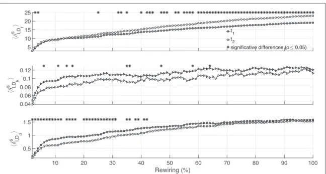
Each network was rewired under the same procedure explained above retrieving∣∣{ }∣∣Al =100perturbed networks to compare with. We repeat this process for 20 independent realizations and then average the distance profiles for each h. Results displayed in figure3suggest that Euclidean distance distinguishes better than the other two metrics the change of alliance patterns among workers observed during the two periods of time t1and

t2.

We assessed the execution time for computing a distances profile for each subject (we used MATLAB R2017a ran in an OS 10.12.6, 4 GHz Intel dual core i7 processor and 32 GB memory). Figure4shows the relatives orders of magnitude in seconds that each metric takes to compute the networks differences. For the analysis of brain connectomes, the average times obtained are: tf=6.83×10−5, td=2.68×10−2, tk=1.90×10−1for the

Euclidean distance, the dissimilarity metric and the kernel-based method, respectively. The results clearly show Euclidean distance as the fastest method in comparison with the others two. Clearly, Dfis 3(4) orders of

magnitude faster than Dd(Dk). Similar relative orders of magnitude are obtained for the social networks.

Runtimefinally determines which measure has the best performance when computing graphs distances.

While the discriminability of Dkis close to that of Df, its runtime is four orders of magnitude slower than Dfdue

to the fact that Dkneeds to search into several scales tofind the highest difference. Ddruntime is three orders of Figure 3. Mean distances profiles dál h,ñfor t1(black) and t2(white) are plotted as a function of the rewired l links (Rewiring %). (a) Euclidean distance yields a discriminability of 60.0%.(b) The kernel-based distance yields a discriminability of 9.0%. In (c) for h=Dd the discriminability is of 33%.

Figure 4. Relative orders of magnitude of execution times for three distance measures. Violin plots show the distributions of all values represented by the small circles. Although time differences between Ddand Dkis around one order, they become slower than Df execution time.

magnitude slower than Df, because Ddtakes into account many topological properties under several tuning

parameters.

To rule out the possibility that the differences in the number of connections of the networks could account for significant differences in the different distances, we have assessed the differences between surrogate graphs of the two groups, obtained by randomly rewiring the links of the original networks while keeping the same degree distribution. This procedure allows‘normalizing’ for the potential influences of changes in the number of connections.

For brain connectomes, we estimate the distance between the aggregate(averaged) network of each group of subjects/patients. For the analysis of social networks, instead, we used the original social interaction matrices. For both dataset we create a set of 100 surrogate networks as described above and compare, by means of a z-value, a given distance between the original networks with that obtained from surrogate pairs.

Table1depicts z-values for the three metrics. Interestingly, the low z-values obtained by Ddsuggest that this

distance mainly reflects differences in the degree distribution. In contrast, the Euclidean and kernel-based distances seem to capture structural differences beyond the degree distribution or density.

In summary, the Euclidean distance emerges as the metric with the highest discriminability to distinguish groups of networks studied here, and the fastest computation, which is something important when one manages large datasets.

3. Concluding remarks

Finding an accurate graph distance is a difficult task, and many metrics have been described without a

framework to properly benchmark such proposals. Here we make a call of the simple Euclidean distance as the one with a very good trade-off between good and fast performances in contrast to more elaborated algorithms. Here we propose a method to detect global network differences with high efficiency and fast computation time. Although we used a random rewiring, the analysis over other perturbations or networks models deserves a statistically detailed study out of the scope of this rapid communication.

Our results suggest a non-trivial dependence between networks’ structure and networks’ distances. Appropriate statistical control of distances(e.g. via group comparisons or random null models) are therefore necessary to take into account these differences. We also propose a simple framework to assess any metric’s performance in terms of discriminability and runtime. Results indicate that, for comparing binary networks of the same size, the Euclidean distance’s discriminating capabilities outperform those of graph dissimilarity and diffusion kernel distance.

Our approach is founded on unweighted network models. Its natural application implies binarization after thresholding, a procedure widely adopted to mitigate the uncertainty carried by the weights estimated from neuroimaging data. Further work is needed to clarify how our approach can be extended to weighted networks, where the perturbation of links is less straightforward(simple rewiring, perturbation of weights, etc). Similarly, more elaborated network models(e.g. multi-layer, signed, spatial, or time-varying networks) might, however, need more elaborated tools to account for the geometry or the interdependencies of interacting units, and make their comparisons more robust.

Acknowledgments

We are indebted to X Navarro, F De Vico Fallani and M D’aubergine for their valuable comments.

ORCID iDs

Johann H Martínez https://orcid.org/0000-0002-3365-8189

Table 1. z-values of different distances for brain and social networks.

Df Dd Dk

Connectomes 13.82 0.18 13.96

Social 9.34 0.98 5.01

6

References

[1] Borgwardt K M, Ong S C, Schönauer R, Vishwanathan S V N, Kriegel H P and Smola A J 2005 ISMB Bioinform.21 47–56 [2] Deshpande M, Kuramochi M, Wale N and Karypis G 2005 IEEE Trans. Knowl. Data Eng.17 1036–50

[3] Ralaivola L, Swamidass S J, Saigo H and Baldi P 2005 Neural Netw.18 1093–110 [4] Simas T, Chavez M, Rodriguez P R and Diaz-Guilera A 2015 Front. Psychol.6 904 [5] Chartrand G, Saba F and Zou H-B 1985 C̆asopis Pĕst. Mat. 110 87–91

[6] Wallis W D et al 2001 Pattern Recognit. Lett.22 701–4 [7] Donnat C and Holmes S 2018 Ann. Appl. Stat.12 971–1012

[8] Wegner A E, Ospina-Forero L, Gaunt R, Deane C and Reinert G 2018 J. Complex Netw.3 cny003

[9] Hammond D K, Gur Y and Johnson C R 2013 2013 IEEE Global Conf. on Signal and Information Processing, GlobalSIP 2013—Proc. vol 3, pp 419–22

[10] Schieber T A, Carpi L, Díaz-Guilera A, Pardanos P M, Massoller C and Ravetti M G 2017 Nat. Commun.8 1–10 [11] Bai L, Rossi L, Torsello H A and Hancock A E 2015 Pattern Recognit.48 1–12

[12] Higham N 2002 Accuracy and Stability of Numerical Algorithms (Philadelphia, PA: Society for Industrial and Applied Mathematics) (https://doi.org/10.1137/1.9780898718027)

[13] Golub G H and Van Loan C F 1996 Matrix Computations (Baltimore, MD: Johns Hopkins University Press) (https://doi.org/10.1137/ 1032141)

[14] Real R and Vargas J M 1996 Syst. Biol.45 380–5 [15] Zelinka B 1975 C̆asopis Pĕst. Mat. 100 371–3

[16] Sanfeliu A and Fu K S 1983 IEEE Trans. Syst. Man Cybern. A13 353–62 [17] Basseville M 1999 Signal Process.18 349–69

[18] Runber Y, Tomasi C and Guibas L J 1998 Proc. 6th Int. Conf. on Computer Vision (ICCV ’98) (IEEE Computer Society)pp 59–66 [19] De Domenico M and Biamonte J 2016 Phys. Rev. X6 041062

[20] Newman M 2010 Networks: An Introduction (Oxford: Oxford University Press) (https://doi.org/10.1093/acprof:oso/ 9780199206650.001.0001)

[21] Lancichinetti A, Fortunato S and Radicchi F 2008 Phys. Rev. E78 046110 [22] Brain Networks Toolboxhttps:_{//github.com/brain-network/bnt}

[23] Guillon J, Attal Y, Colliot O, Schwartz D, Chavez M and De Vico Fallani F 2017 Nat. Sci. Rep.7 1_–13

[24] Stam C J, Van Walsum A M V C, Pijnenburg Y A, Berendse H W, De Munck J C, Scheltens P and Van Dijk B W 2002 J. Clin. Neurophysiol.19 562–74

[25] De Vico Fallani F, Latora V and Chavez M 2017 PLoS Comput. Biol.13 1–18

[26] De Vico Fallani F, Richiardi J, Chavez M and Achard S 2014 Phil. Trans. R. Soc. B369 20130521

[27] Kapferer B 1972 Strategy and Transaction in an African Factory: African Workers and Indian Management in a Zambian Town (Manchester: Manchester University Press) (https://doi.org/10.2307/1159273)