Lorentz Force Electrical Impedance Tomography

HAL Id: inserm-00920558

https://www.hal.inserm.fr/inserm-00920558

Submitted on 18 Dec 2013

HAL is a multi-disciplinary open access

archive for the deposit and dissemination of

sci-entific research documents, whether they are

pub-lished or not. The documents may come from

teaching and research institutions in France or

abroad, or from public or private research centers.

L’archive ouverte pluridisciplinaire HAL, est

destinée au dépôt et à la diffusion de documents

scientifiques de niveau recherche, publiés ou non,

émanant des établissements d’enseignement et de

recherche français ou étrangers, des laboratoires

publics ou privés.

Lorentz Force Electrical Impedance Tomography

Pol Grasland-Mongrain, Jean-Martial Mari, Jean-Yves Chapelon, Cyril Lafon

To cite this version:

Pol Grasland-Mongrain, Jean-Martial Mari, Jean-Yves Chapelon, Cyril Lafon. Lorentz Force Electrical

Impedance Tomography. Innovation and research in biomedical engineering, 2013, 34 (5-6),

pp.357-360. �inserm-00920558�

Lorentz Force Electrical Impedance Tomography

Pol Grasland-Mongrain

_{, Jean-Martial Mari}

_{, Jean-Yves Chapelon}

_{, Cyril Lafon}

R´esum´e— This article describes a method

cal-led Lorentz Force Electrical Impedance Tomo-graphy. The electrical conductivity of biologi-cal tissues can be measured through their so-nication in a magnetic field : the vibration of the tissues inside the field induces an electrical current by Lorentz force. This current, detec-ted by electrodes placed around the sample, is proportional to the ultrasonic pressure, to the strength of the magnetic field and to the elec-trical conductivity gradient along the acoustic axis. By focusing at different places inside the sample, a map of the electrical conductivity gradient can be established. In this study expe-riments were conducted on a gelatin phantom and on a beef sample, successively placed in a 300 mT magnetic field and sonicated with an ultrasonic transducer focused at 21 cm emit-ting 500 kHz bursts. Although all interfaces are not visible, in this exploratory study a good correlation is observed between the electrical conductivity image and the ultrasonic image. This method offers an alternative to detecting pathologies invisible to standard ultrasonogra-phy.

Mots-Cl´es

Medical Imaging, Electrical Conductivity Ima-ging, Magneto-Acousto-Electrical Tomography, Ultrasonically-Induced Lorentz Force, Lorentz Force Electrical Impedance Tomography, Hall Effect Imaging

I. INTRODUCTION

The electrical conductivity of biological tissues arouses great interest for medical imaging researchers. Indeed this parameter potentially shows a good contrast in the human body. For example, fat is ten times less conductive than muscle tissue [5] while the acous-tic impedance, observed in ultrasonography , only changes of a few percents through the soft tissues. Electrical conductivity anomalies can moreover reveal pathologies like tumors [8].

The most advanced technique today to measure the electrical conductivity of tissue is the Electrical Impe-dance Tomography (EIT) [3]. In this technique, seve-ral electrodes are placed around the body or the organ

under study. An electrical current is injected through each electrode while its distribution in the tissues is measured by the others. These measurements allow an electrical impedance image reconstruction through mathematical analysis. This apparently simple and in-expensive technique suffers however of a low spatial resolution due to the intrinsic ill-posed nature of the mathematical problem [2].

On another hand, the vibration of a conductor inside a magnetic field induced by ultrasound induces by Lo-rentz force an electrical current which is connected to the electrical conductivity of the conductor [4]. This approach can be applied to the measurement of ultra-sound velocity using a wire as sensing element, for its electrical conductivity is known [6], [7]. Conversely,the ultrasound pressure distribution in the conductor is known [14], the electrical conductivity could be dedu-ced . In this last approach, the biological tissues are submitted to a magnetic field created for example by a permanent magnet, and a focused ultrasound beam is used to vibrate the tissues in a specific region of inter-est [13]. In the same way the movement of a conductor in a magnetic field would induce an electrical current, this vibration induces a current in the tissues which can be detected by the mean of electrodes. The fo-cusing of ultrasound allows conferring to the imaging process an important characteristic when compared to Electrical Impedance Tomography : the spatial reso-lution is close to the one that would be reached by ultrasound imaging. However, the drawback of such approach lies in the weakness of the induced electrical current. The initial name of the technique, the Hall Effect Imaging [21] was criticized later on as the phe-nomenon is not exactly an Hall Effect [18],. The tech-nique has also been called Magneto-Acousto-Electrical Tomography [9] or scan of electric conductivity gra-dients with ultrasonically-induced Lorentz force [16]. We use here the name of Lorentz Force Electrical Im-pedance Tomography (LFEIT), which has the advan-tage of describing both the imaged parameter and the method.

II. THEORY

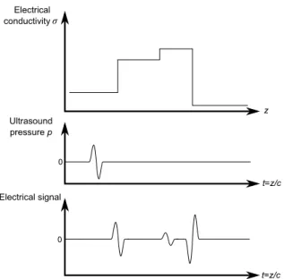
For clarity reasons, the X axis is defined as the orien-tation of the magnetic field, the Z axis is defined along the ultrasound propagation direction and the Y axis is placed accordingly using the right-hand rule. As

expo-z t=z/c Electrical conductivity Ultrasound pressure p 0 Electrical signal t=z/c 0 σ

Figure_{1 – The electrical signal detected by electrodes} in Lorentz Force Electrical Impedance Tomography is proportional to the convolution product between elec-trical conductivity gradients and the ultrasound pres-sure shape.

sed previously, the Lorentz Force Electrical Impedance Tomography is based on the movement of a conductor placed inside a magnetic field, which induces an elec-trical current. Physical and mathematical modellings have been proposed to describe the method [1], [20]. We choose here the model presented by Montalibet et al. which gives a good understanding of the phenome-non [17]. In this model, the induced current is found to be proportional to the convolution product of the electrical conductivity gradient H with the ultrasound pressure shape P : i(t) = Z (dσ dz B ρ) ∗ ( Z t 0 p(τ )dτ )dS = c(H ∗ P )(t) (1) with i the induced electrical current, dσ

dz the

electri-cal conductivity gradient along z axis, B the magnetic field, ρ the density, p the ultrasound pressure and c the speed of sound.

In other words, the electrical current detected by the electrodes is a temporal image of the ultrasound pulse at each electrical conductivity interface, as shown by the figure (1). More refined models are however avai-lable [1], [20].

III. MATERIALS AND METHODS

The goal of this study was to build a setup to produces LFEIT images of gelatine phantoms and biological tis-sues.

The experiment setup is illustrated in figure (3). A ge-nerator (HP33120A, Agilent, Santa Clara, CA, USA)

Position Z (mm) P os iti on X (m m ) 0 50 100 150 200 250 300 350 400 −40 −20 0 20 40 MPa 0 1 2 3

Figure_{2 – Pressure field simulation along ultrasound} axis (Y = 0 mm) of the transducer. The maximum of pressure is approximately at 15 cm of the transducer.

created 0.5 MHz, 3 cycles sinusoid bursts at a pulse repetition frequency of 100 Hz. This excitation was amplified by a 200 W linear power amplifier (200W LA200H, Kalmus Engineering, Rock Hill, SC, USA) and sent to a 0.5 MHz, 50 mm in diameter transducer focused at 210 mm and placed in a 100x50x50 cm3

degassed water tank.

The ultrasound pressure was equal to 3 MPa at the focal point (Z = 210 mm). A simulation of the ul-trasound pressure field based on the resolution of the linear Rayleigh equation is shown in figure (2). A 20x4x15 cm3

mineral oil tank was placed from 15 to 35 cm away from the transducer in the ultrasound beam axis. This oil tank was placed in the middle of a U-shaped permanent magnet, composed of two poles made of two 5x5x3 cm3 NdFeB magnets (BLS Magnet, Villers la Montagne, France). The gap between the poles was 4.5 cm. The magnetic field was equal to 90 mT in a 4 cm radius circle around the maximum of 340 mT.

The tested sample was placed inside this tank from 22 to 28 cm of the transducer. Two samples were tested : a phantom made of 10% gelatin and 1% salt, 8 cm wide, as shown in figure (4) ; and a 6 cm wide piece of beef muscle with an L-shape, having a fat layer in the middle of the sample, as shown in figure (5). A pair of 10x3x0.1 cm3

copper electrodes was placed in contact with the sample, respectively above and un-der it. The electrodes were linked through an electri-cal wire to a 1 MV/A current amplifier (HCA-2M-1M, Laser Components, Olching, Germany) and an oscil-loscope with 50 Ω input impedance (WaveSurfer 422, LeCroy, Chestnut Ridge, NY, USA) which was avera-ging the measures over 5000 acquisitions. The signals were post-processed using the Matlab software (The MathWorks, Natick, MA, USA) by computing the Hil-bert transform modulus of the signal and converting it into a line of color.

The ultrasound signal was simultaneously recorded from the echoes on the transducer.

IV. RESULTS

The figure (6) shows respectively the ultrasound image and the electrical impedance image of the gelatin

absorber sample with electrodes magnet (300 mT) transducer (500 kHz) oil tank degassed water

Figure _{3 – A transducer is emitting ultrasound in a} sample placed in an oil tank in the middle of a magne-tic field. The induced electrical current is received by two electrodes.

Figure_{4 – Photo of salty gelatin sample. The sample} is made of 2 blocks, one of 8x2x2 cm3

under the second of 4x2x3 cm3

. Two electrodes are in contact above and under the sample. Arrows are indicating front and back interfaces.

phantom. The front and back interfaces are equally visible on both images. The relative amplitude of in-terface signal is however different, mostly due to ma-gnetic field inhomogeneity.

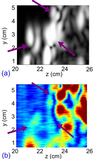
The figure (7) shows respectively the ultrasound image and the electrical impedance image of the beef sample. The front interface can be seen on both images, al-though the lower one is less visible.

V. DISCUSSION AND CONCLUSION A method to observe electrical conductivity gradients by combining ultrasound and magnetic field is tested experimentally.

The tested transducer is a standard single element ultrasonic therapy transducer. The magnetic field is created by a permanent magnet with sufficient air gap to insert a tissue sample. The signal has been shown to be little influenced by the electrodes posi-tions [15]. The oil bath prevents any electrical contact between the sample and the transducer ; in practi-cal applications it could easily be placed around the

Figure_{5 – Photo of beef sample. The sample has an} L-shape, 6 cm wide, 2 cm large and 6 cm high. Two electrodes are in contact above and under the sample. Squares are 5 mm wide. Arrows are indicating two front interfaces and the fat layer.

transducer rather than around the patient. The ex-periment showed images of quality comparable to the one of the ultrasound images taken in the same condi-tions. The combination of ultrasonography and Lo-rentz Force Electrical Impedance Tomography with ultrasonically-induced Lorentz force can be made ea-sily with the same material. Elements like fat layers which are hardly visible here in the ultrasonic image can be observed in the Lorentz Force Electrical Im-pedance Tomography image. The technique has po-tentially the spatial resolution of the ultrasound wa-velength [12], allowing the observation of small inho-mogeneities and can help thus revealing pathologies like cancer by detecting tumorous tissues where other techniques fail to do so.

Image quality could be improved with a higher ultra-sound frequency and a thinner beam. The compatibi-lity of ultrasound imaging with MRI [10] shows that it is possible to use much stronger magnetic fields, which would increase the intensity of the induced electrical current, and thus the signal to noise ratio. Moreover, even if the magnetic field homogeneity is not as cri-tical in this technique as in MRI [16], a more homo-geneous magnetic field would provide sharper images of the interfaces. The technique can also be used in a reverse mode [21], with an electrical current applied in a tissue submitted to a magnetic field, which leads to ultrasound wave [22] and was recently applied to hu-man tissue ex-vivo [11]. It is nevertheless hard to say which of these techniques would be the most useful for biomedical imaging [19].

20 24 28 2 1 0

z (cm)

y

(cm

)

(a)

z (cm)

y

(cm

)

(b)

Figure _{6 – (a) Ultrasound image of the gelatin} sample. (b) Electrical impedance image of the gelatin sample. Arrows are indicating the interfaces shown on the photograph.

VI. ACKNOWLEDGMENTS

The authors would like to thank Amalric Montalibet for its pioneer work on the subject, R´emi Souchon for his advices and Alexandre Petit for theory sug-gestions.No conflict of interest is declared.

R´EF´ERENCES

[1] Habib Ammari, Yves Capdeboscq, Hyeonbae Kang, Anastasia Kozhemyak, et al. Mathematical models and reconstruction methods in magneto-acoustic imaging. Euro. J. Appl. Math, 20 :303– 317, 2009.

[2] Habib Ammari and Hyeonbae Kang. Reconstruc-tion of small inhomogeneities from boundary mea-surements. Springer, 2004.

[3] Margaret Cheney, David Isaacson, and Jona-than C Newell. Electrical impedance tomography. SIAM review, 41(1) :85–101, 1999.

[4] Leszek Filipczynski. Absolute measurements of particle velocity, displacement or intensity of ul-trasonic pulses in liquids and solids. Acustica, 21 :173–180, 1969.

[5] Camelia Gabriel, Sami Gabriel, and E Corthout. The dielectric properties of biological tissues : I. literature survey. Physics in medicine and biology, 41(11) :2231, 1996.

[6] Pol Grasland-Mongrain, Jean-Martial Mari, Bruno Gilles, Jean-Yves Chapelon, and Cyril

La-3

2

1

4

5

z (cm)

y

(cm

)

20

22

24

26

(a)

3

2

1

4

5

20

22

24

z (cm)

26

y

(cm

)

(b)

Figure_{7 – (a) Ultrasound image of the beef sample.} (b) Electrical impedance image of the beef sample. Ar-rows are indicating the interfaces shown in the photo-graph.

fon. Electromagnetic hydrophone with tomogra-phic system for absolute velocity field mapping. Applied Physics Letters, 100(24) :243502–243502, 2012.

[7] Pol Grasland-Mongrain, Jean-Martial Mari, Bruno Gilles, and Cyril Lafon. Electromagnetic hydrophone for high-intensity focused ultrasound (hifu) measurement. Proceedings of Meetings on Acoustics, 2013 (in press).

[8] Dieter Haemmerich, ST Staelin, JZ Tsai, S Tung-jitkusolmun, DM Mahvi, and JG Webster. In vivo electrical conductivity of hepatic tumours. Phy-siological measurement, 24(2) :251, 2003.

[9] S Haider, A Hrbek, and Y Xu. Magneto-acousto-electrical tomography : a potential method for imaging current density and electrical impedance. Physiological measurement, 29(6) :S41, 2008.

[10] Pascal Haigron, Jean-Louis Dillenseger, Limin Luo, and Jean-Louis Coatrieux. Image-guided therapy : evolution and breakthrough [a look at]. Engineering in Medicine and Biology Magazine, IEEE, 29(1) :100–104, 2010.

[11] Gang Hu, Erik Cressman, and Bin He. Magne-toacoustic imaging of human liver tumor with magnetic induction. Applied physics letters, 98 :023703, 2011.

[12] MR Islam and BC Towe. Computer image recons-truction of bioelectric currents from magneto-acoustic measurements. In Engineering in Me-dicine and Biology Society, 1988. Proceedings of the Annual International Conference of the IEEE, pages 441–442. IEEE, 1988.

[13] Jean Martial Mari, Thierry Blu, Olivier Bou Ma-tar, Michael Unser, and Christian Cachard. A bulk modulus dependent linear model for acous-tical imaging. The Journal of the Acousacous-tical So-ciety of America, 125 :2413, 2009.

[14] Jean Martial Mari, Kathryn Hibbs, Eleanor Stride, Robert J Eckersley, and Meng Xing Tang. An approximate nonlinear model for time gain compensation of amplitude modulated images of ultrasound contrast agent perfusion. Ultraso-nics, Ferroelectrics and Frequency Control, IEEE Transactions on, 57(4) :818–829, 2010.

[15] Amalric Montalibet. Etude du couplage acousto-magn´etique : d´etection des gradients de conducti-vit´e ´electrique en vue de la caract´erisation tissu-laire. PhD thesis, Institut Nationale des Sciences Appliqu´ees de Lyon, 2002.

[16] Amalric Montalibet, Jacques Jossinet, and Adrien Matias. Scanning electric conducti-vity gradients with ultrasonically-induced lorentz force. Ultrasonic imaging, 23(2) :117–132, 2001. [17] Amalric Montalibet, Jossinet Jossinet, Adrien

Matias, and Dominique Cathignol. Electric cur-rent generated by ultrasonically induced locur-rentz force in biological media. Medical and Biological Engineering and Computing, 39(1) :15–20, 2001. [18] B.J. Roth, Jr. Wikswo, J.P., Han Wen, and R.S.

Balaban. Comments on ”hall effect imaging” [with reply]. Biomedical Engineering, IEEE Tran-sactions on, 45(10) :1294–1296, 1998.

[19] Bradley J Roth. The role of magnetic forces in biology and medicine. Experimental Biology and Medicine, 236(2) :132–137, 2011.

[20] Bradley J Roth, Peter J Basser, and John P Wikswo. A theoretical model for magneto-acoustic imaging of bioelectric currents. IEEE transactions on biomedical engineering, 41(8) :723–728, 1994.

[21] Han Wen, Jatin Shah, and Robert S Balaban. Hall effect imaging. Biomedical Engineering, IEEE Transactions on, 45(1) :119–124, 1998. [22] Yuan Xu and Bin He. Magnetoacoustic

tomogra-phy with magnetic induction (mat-mi). Physics in medicine and biology, 50(21) :5175, 2005.