HAL Id: hal-03086120
https://hal.uca.fr/hal-03086120
Submitted on 22 Dec 2020
HAL is a multi-disciplinary open access archive for the deposit and dissemination of sci-entific research documents, whether they are pub-lished or not. The documents may come from teaching and research institutions in France or abroad, or from public or private research centers.
L’archive ouverte pluridisciplinaire HAL, est destinée au dépôt et à la diffusion de documents scientifiques de niveau recherche, publiés ou non, émanant des établissements d’enseignement et de recherche français ou étrangers, des laboratoires publics ou privés.
Distributed under a Creative Commons Attribution| 4.0 International License
Euler-Euler large eddy simulations of the gas–liquid flow
in a cylindrical bubble column
Mojtaba Goraki Fard, Youssef Stiriba, Bouchaib Gourich, Christophe Vial,
Francesc Xavier Grau
To cite this version:
Mojtaba Goraki Fard, Youssef Stiriba, Bouchaib Gourich, Christophe Vial, Francesc Xavier Grau. Euler-Euler large eddy simulations of the gas–liquid flow in a cylindrical bubble column. Nuclear Engineering and Design, Elsevier, 2020, 369, pp.110823. �10.1016/j.nucengdes.2020.110823�. �hal-03086120�
Euler-Euler large eddy simulations of the gas-liquid flow in a
cylindrical bubble column
Mojtaba Goraki Fard
1, Youssef Stiriba
1, *, Gourich Bouchaib
2, Christophe Vial
3, Francesc
Xavier Grau
11
ETSEQ, Departament d’Enginyeria Mecanica, Universitat Rovira i Virgili
Av. Paisos Catalans 26, 43007, Tarragona, Spain
2 Laboratoire d’Ingénierie des Procédés et d’Environnement, Ecole Supérieure de Technologie, Université Hassan II de Casablanca, Route del Jadida, km 7, BP 8012, Oasis Casablanca, Morocco
3 Université Clermont Auvergne, Institut Pascal, 2 Avenue Blaise Pascal, TSA 60206, CS 60026, 63178, Aubière Cedex, France
Abstract
In this work Euler-Euler Large Eddy Simulations (LES) of dispersed turbulent gas-liquid flows in a cylindrical bubble column are presented. Besides, predictions are compared with experimental data from Vial et al. 2000 using laser Doppler velocimetry (LDV). Two test cases are considered where vortical-spiral and turbulent flow regimes occur. The sub-grid scale (SGS) modelling is based on the Smagorinsky kernel with model constant 𝐶𝑠= 0.08 and the one-equation model for SGS kinetic energy. The emphasis of this work is to analyse the performance of the one-equation SGS model for the prediction of bubbly flow in a three-dimensional high aspect ratio bubble column (𝐻 𝐷⁄ ) of 20 and the investigation of the influence of the superficial gas velocity using the OpenFOAM package. The model is compared with the Smagorinsky SGS model and the mixture 𝑘 − 𝜀 model in terms of the axial liquid velocity, the gas hold-up and liquid velocity fluctuations. The bubble induced turbulence and various interfacial forces including the drag, lift, virtual mass and turbulent dispersion where incorporated in the current model. Overall, the predictions of the liquid velocities are in good
agreement with experimental measurement using the one-equation SGS model and the Smagorinsky model which improve the mixture 𝑘 − 𝜀 model in the core and near-wall regions. However, small discrepancies in the gas hold-up are observed in the bubble plume region and the mixture 𝑘 − 𝜀 model performs much better. The numerical simulations confirm that the energy spectra of the resolved liquid velocities in churn-turbulent regime follows the classical -5/3 law for low frequency regions and close to -3 for high frequencies. More details of the instantaneous local flow structure have been obtained by the Euler-Euler LES model including large-scale structures and vortices developed in the bubble plume edge.
Keywords:
Bubble column; Euler-Euler model; Large eddy simulation; One-equation SGS model1. Introduction
Bubbly gas-liquid flows in multiphase reactors are important for many industrial processes, for instance in the chemical, biochemical, or environmental industries and have advantageous characteristics in mass and heat transfers. In bubble column reactors, the gas phase is dispersed in the form of tiny bubbles in a continuous liquid phase using a gas distribution device. The complex interplay between operating conditions, the gas-liquid interfacial area, bubble size, bubble rise velocity, turbulence in the liquid phase, and bubble-bubble interactions lead to extensive range of flow regimes and complex flow structures. Furthermore, as the bubbles rise in the column, they induce pseudo-turbulence in the liquid phase. Several numerical studies of these types of flows have been carried out by incorporating the turbulence of the liquid phase through the Reynold-Averaged Navier-Stokes (RANS) model (Mudde and Simonin, 1999; Plfeger and Becker, 2001; Tabib et al., 2008; Olmos et al., 2001; Selma et al., 2010; Stiriba et al., 2017; Kouzbour et al., 2020). The RANS approach, typically the 𝑘 − 𝜀 model, models the effect of liquid turbulence on the mean flow scale
and uses isotropic closures, but fails to reproduce relevant flow physics since bubbles induce significant turbulence of anisotropic nature. It has provided valuable results and insights on the turbulence in bubble column reactors with reasonable computational costs.
Bubbly flow is characterised by the development of distinct flow structures of different length scales, especially for transition and heterogeneous flow regimes. Turbulent scales varied from those of the characteristic length of the mean flow to those of the microscopic ones. For instance, the largest turbulence scales are comparable in size to those of the mean flow and depend on the reactor geometry and flow conditions, whereas the smallest scales depend on the bubble dynamics and are proportional to the bubble size.The large-scale turbulent motions interact with the bubbles and thereby affect their motions, whereas the small scales are proportional to the bubble diameter and not only dissipate the kinetic energy but can generate energy to the largest scales and tend to be more isotropic as well (Dhotre et al., 2013 and Ma et al., 2015). The energy spectra of the liquid fluctuations exhibit a broad range of frequency and gives a power law scaling with the slope of -5/3 for low frequency regions which is progressively replaced by -25/3 in Lui et al. 2018 and over than -8/3 in the works of Ma et al. 2015 and Lance and Bataille 1991 for high frequency regions.
To reproduce relevant flow physics and give comprehensive insights of two-phase flow turbulence, the LES approach has attracted great attention in the simulation of dispersed two-phase turbulent flows. It has been used in several investigations and simulations to predict multiphase flow dominated by large coherent structures or eddies in bubble columns, stirred tanks and many other reactors (Tabib et al., 2011; Dhotre et al., 2008). As in single phase flows, LES model resolves directly the interaction of the large-scale motions with bubbles, whereas the less energetic smallest motions including the interaction of the bubbles with the surrounding turbulence are represented in terms of sub-grid scale closure models. The Euler-Euler LES model predicts more accurately flows dominated by large coherent structures or eddies in bubble columns which carry most of the flow energy (typically 90%)than the traditional RANS models both the liquid velocity and the
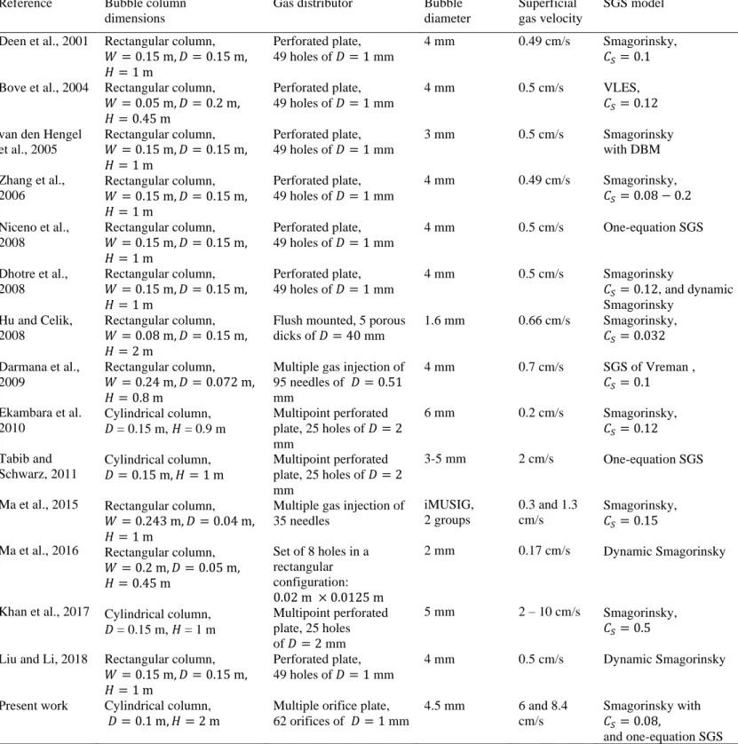
bubble-induced velocity fluctuations in the liquid as well as represents more details of the flow structure (Ma et al., 2015; Dhotre et al. 2008). Furthermore, the 𝑘 − 𝜀 models consider isotropic turbulence and do not analyse the flow near the walls. Table 1 gives a summary of previous works of gas-liquid flows in bubble column reactors in a chronological manner. For instance, Zhang et al. (Zhang et., 2006) investigated the Smagorinsky model with different values of the constant 𝐶𝑠 and the dynamic Smagorinsky model. Niceno et al. 2008 applied the one-equation SGS turbulent kinetic energy LES and suggested that the sub-grid scale kinetic energy obtained from the model can be used to assess the SGS dispersion turbulent force. Tabib et al. (Tabib et al., 2011) employed the commercial CFD package ANSYS CFX to analyse the inclusion of SGS turbulent dispersion (TD) force and concluded that the results of coarser mesh can be improved by using a lower magnitude of SGS-TD force. Liu et al. 2018 studied the scale-adaptive of LES with small ∆ 𝑑⁄ 𝐵 ≤ 1 with ANSYS CFX code. These works have made several assumptions in the CFD modelling, reactor geometry and operating conditions. Indeed, the bubble columns are operating at low superficial gas velocities with non-uniform aerations or use flat bubble column reactors. At high gas flow rates, the flow field is unsteady and characterized by local recirculation near the sparger and different scale vortices at the core region.
In view of this, it is desirable to carry out LES in a three-dimensional bubble column at high inlet superficial gas velocity. The purpose of this work is therefore to employ Euler-Euler LES approach to simulate dispersed turbulent two-phase flows in a three-dimensional cylindrical bubble column of high aspect ratio (𝐻 𝐷⁄ ) of 20 with special emphasis on the performance of the one-equation SGS model and the influence of the superficial gas velocity. A multiple gas distributor is used for uniform aeration. The inlet superficial gas velocities, used in this work, are 𝑈𝐺 = 6 and 8.4 cm/s where vortical-spiral and turbulent flow regimes occur, respectively. The simulations are set up according to experimental works of Vial et al. (2000) using LDA as well as they have been performed by using the twoPhaseEulerFoam solver implemented in the OpenFOAM v3.0.1 software package. The results achieved from the one-equation model SGS are compared with the Smagorinsky model with constant
𝐶𝑠= 0.08 and the mixture 𝑘 − 𝜀 model. The accuracy of the results in comparison to experimental data are evaluated. Comprehensive simulations were conducted to examine the instantaneous flow structure and Reynolds stresses. Further, the analysis of the energy spectra of resolved velocity and the vorticity distribution have been carried out.
2. Two fluid model and numerical setup
2.1. The flow equations
The two-fluid model is built up on the spatial filtering for LES or conditional averaging for RANS of the conservation equations of mass and momentum. In this approach, both phases, the continuous liquid phase and the dispersed gas phases, are modelled as two interpenetrating continua. In LES cases, it is assumed that the filtered equations are used to compute the large-scale lengths while the effect of unresolved turbulent scales are modelled using a sub-grid model. In the present work, the flow is assumed to be adiabatic, without the consideration of the interfacial mass transfer between the air and the water phases.
The present formulation closely follows the procedure outlined by Weller 2005, where the mass and momentum equations for the phase 𝜑 are given by
𝜕(𝜌
𝜑𝛼
𝜑)
𝜕𝑡
+ ∇ ∙ (𝜌
𝜑𝛼
𝜑𝐔
𝜑) = 0
𝜕(𝜌
𝜑𝛼
𝜑𝐔
𝜑)
𝜕𝑡
+ ∇ ∙ (𝜌
𝜑𝛼
𝜑𝐔
𝜑𝐔
𝜑) = −𝛼
𝜑∇𝑝
𝜑+ 𝛼
𝜑𝜌
𝜑𝐠 − ∇ ∙ (𝛼
𝜑𝜌
𝜑𝛕
𝜑 eff) + 𝐌
𝜑Here 𝛼𝜑 is the volume fraction of each phase, 𝐔𝜑 is the phase resolved velocity, and 𝜏𝜑eff represents the effective stress tensor usually decomposed into a mean viscous stress and turbulent stress tensor for phase 𝜑 as
(1)
𝛕
𝜑eff= −𝜈
𝜑eff[∇𝐔
𝜑+ (∇𝐔
𝜑)
𝑇−
2
3
(∇ ∙ 𝐔
𝜑)𝐈] +
2
3
𝑘
𝜑𝐈
where 𝑘𝜑 is the turbulent kinetic energy of phase 𝜑, 𝐈 is the identity tensor, and 𝜈𝜑𝑒ff is the effective viscosity of phase 𝜑. The effective viscosity of the liquid phase is obtained through the summation of the molecular viscosity, the shear-induced turbulent viscosity, and the bubble-induced turbulent viscosity
and is formulated in the present study using two models: (a) the Smagorinsky model proposed by Zhang et al. (2006), (b) and the one-equation sub-grid-scale model proposed by Niceno et al. (2008).
The Smagorinsky model is a zero-equation turbulent LES model and the liquid phase shear-induced turbulent viscosity is formulated as follows
Here 𝐶𝑆 is a model constant, 𝑆 is the characteristic filtered rate of the strain and ∆= 𝑉𝑜𝑙1 3⁄ is the filtered width, where 𝑉𝑜𝑙 is the volume of the computational cell. The model constant seems to be different for different flow situation and was chosen to be 𝐶𝑆≈ 0.1 according to the work of Zhang et al. 2006. The turbulence model corrects the SGS turbulent viscosity by a contribution due to the bubble induced turbulence, see Zhang et al. 2006. The model proposed by Sato and Sekoguchi (Sato and Sekoguchi, 1975) was employed
with its constant 𝐶𝜇,BIT set to 0.6.
The one-equation sub-grid-scale model by Niceno et al. (2008) solves a transport equation for the unresolved kinetic energy 𝑘𝑆𝐺𝑆. The model is able to account for the effects of bubble induced turbulence through an additional source term in the transport equation for 𝑘𝑆𝐺𝑆 in the continuous (3)
𝜈𝜑eff= 𝜈𝐿,𝐿+ 𝜈𝐿,Tur+ 𝜈𝐿,BIT (4)
𝜈𝐿,Tur = (𝐶𝑆∆)2|𝑆| (5)
phase and uses the modelled SGS energy to estimate the SGS turbulent dispersion force (Niceno et al., 2008). The sub-grid kinetic energy equation is given by
where 𝐺 is the production term, defined as
and the sub-grid viscosity is
The model constants are 𝐶𝜀= 1.05 and 𝐶𝑘 = 0.07 (Niceno et al., 2008).
In Eq. (2), 𝐌𝜑 represents the inter-phase momentum exchange between phase 𝜑 and the other phase due to various interphase forces. The interfacial forces are decomposed into four contributions
where the forces on the right-hand side of equality are the drag force denoted by 𝐌𝜑𝐷, the lift force represented by 𝐌𝜑𝐿, the virtual mass force by 𝐌
𝜑
𝑉𝑀, and the turbulent dispersion force by 𝐌 𝜑
𝑇𝐷. There are many models for each of these forces depending on their applicability, the flow regime and the operating conditions as discussed by (Joshi, 2001; Vial and Stiriba, 2013; and Ziegenhein et al., 2015). There is still no complete agreement on the closures or the combination to be used at best. The drag force (per volume) for the liquid phase is estimated as
(10) 𝜕𝑘𝑆𝐺𝑆 𝜕𝑡 + ∇ ∙ (𝑘𝑆𝐺𝑆𝐔) − ∇ ∙ [(𝜈𝐿,𝐿+ 𝜈𝑆𝐺𝑆)∇𝑘𝑆𝐺𝑆] = 𝐺 − 𝐶𝜀 𝑘𝑆𝐺𝑆3 2⁄ ∆ 𝐺 = 𝜈𝑆𝐺𝑆|𝑆̅𝑖𝑗| 𝜈𝑆𝐺𝑆= 𝐶𝑘∆𝑘𝑆𝐺𝑆1 2 ⁄ (8) (9) (7)
𝐌
𝜑= 𝐌
𝜑𝐷+ 𝐌
𝜑𝐿+ 𝐌
𝜑𝑉𝑀+ 𝐌
𝜑𝑇𝐷 𝐌𝐿𝐷= 3 4𝛼𝐺𝜌𝐿 𝐶𝐷 𝑑𝐵 |𝐔𝑟|𝐔𝑟 (11)where 𝐶𝐷 refers to the drag force coefficient and is calculated according to the Schiller-Neumann correlation and 𝐔𝑟 is the relative velocity. Many drag model have been proposed and compared in the literature (Pourtousi et al., 2014; Tabib et al., 2008; Zhang et al., 2006; and Silva et al., 2012). For instance, Tabib et al. 2008 who found that Schiller-Naumann, Ishii-Zuber, Tomiyama, and Grace et al. using different turbulence closure (𝑘 − 𝜀, RNG, LES) models give the same results in a cylindrical bubble column similar to our reactor. Furthermore, the Schiller-Naumann drag model works quite well for bubbly flow in industrial systems since bubbles are contaminated by surfactants at the interface and behaves like a rigid sphere (Clift et al. 1979).
The lift force results from the movement of bubbles through a non-uniform flow field due to shear or vorticity effects. The force (per volume) is modelled as
where 𝐶𝐿 is a constant lift force. We conducted the same simulation with different lift coefficients and the model of Tomiyama et al. (2002), but no noticeable improvements in the results was observed, from which we conclude that the lift force plays a minor role in our test cases. Furthermore, the steady simulations of a bubble column reactor (Vial and Stiriba, 2013), the use of the lift force overestimates the radial dispersion of the bubbles, as it does not better predict the experimental gas holdup at the column center.
Liquid acceleration in the wake of the bubble is taking into account through the virtual mass force, which is modelled as
where 𝐶𝑉𝑀 is the virtual mass coefficient and is taken to be 0.5 for individual spherical bubbles (Zhang et al., 2006; Dhotre et al., 2008).
𝐌𝐿𝐿= 𝛼 𝐺𝜌𝐿𝐶𝐿𝐔𝑟× (∇ × 𝐔𝑟) (12) 𝐌𝐿𝑉𝑀= 𝛼𝐺𝜌𝐿𝐶𝑉𝑀( 𝐷𝐔𝐿 𝐷𝑡 − 𝐷𝐔𝐺 𝐷𝑡 ) (13)
The SGS component of those forces will be neglected except the turbulent dispersion force which can be estimated using the modelled SGS energy in the one-equation model. The turbulent dispersion force proposed by Lopez de Bertodano et al. (1994) is adopted. It is modelled as
Several turbulent dispersion coefficients 𝐶𝑇𝐷, required to obtain good agreement with experimental measurements, were tested. For the one-equation and mixture 𝑘 − 𝜀 models we use 𝐶𝑇𝐷= 0.6.
2.2 Numerical simulation set-up
The numerical simulations were carried out in a cylindrical bubble column with uniform aeration. The geometry of the current bubble column reactor is the same as used by Vial et al. (2001) and 2002 in their experiments. The height of the column is 𝐻 = 2 m, the diameter is 𝐷 = 0.10 m, and the static liquid height is 1.35 m. The reactor is operated with the water and air as the continuous and dispersed phases at the room temperature and atmospheric pressure, respectively, at two superficial gas velocities 6 cm/s and 8.4 cm/s corresponding to transition and heterogeneous flow regimes. The gas is injected from the bottom of the column through a multiple-orifice nozzle for uniform aeration and it allow us to study the flow regime transition. The gas distributor is treated as a uniform mass flow rate through the bottom boundary calculated from superficial gas velocities for mass conservation with gas volume fraction of 1.0. The pressure at the inlet is set to zeroGradient and specified by zero gradient. At the outlet, the pressure is specified as the atmospheric pressure, and the gas hold up is set to inletOutlet with zero gradient for outflow and fixed value for backward flow. The no-slip condition is applied at the walls for the velocities and Dirichlet condition for the gas hold-up. Moreover, for the one-equation model we apply wall functions.
The numerical simulations were carried out with the open source CFD package OpenFOAM library (Weller et al., 1998). The governing equations of continuity and momentum as well as the transport equation for 𝑘𝑆𝐺𝑆 are solved by the two-phase flow solver twoPhaseEulerFoam available in
OpenFOAM 3.0.1. The solver is based on a finite volume formulation to discretise the model equations which has shown to be stable for transient calculations (Weller, 2005). The first-order bounded implicit Euler scheme is adopted for the time integration, the gradient terms are approximated with a linear interpolation, the convective terms are discretized with second-order upwind scheme, and the diffusive terms are interpolated with the Gauss linear orthogonal scheme. we employ the PIMPLE algorithm to solve the pressure-velocity coupling where the pressure equation is solved, and the predicted velocities are corrected by the pressure change. The preconditioned conjugate gradient (PCG) is used for solving the discretized pressure equation and the incomplete-Cholesky preconditioned bi-conjugate gradient (BICCG) for the other set of linear equations. For more detailed discussions of all steps mentioned above (Rusche, 2002; Weller, 2005).
Prior to the description of the computational mesh and presenting the results, we emphasis the implications of bubble size distribution on the model. In the present work, we assume a spherical bubble size distribution of 4.5 mm according to bubble size measurements of Vial et al. (2001). The same simplification was successfully used by Khan et al. (2017) to simulate their bubble column using 𝑘 − 𝜀, RSM, and Smagorinsky turbulence model at high superficial gas velocities. Perhaps the incorporation of bubble coalescence and break up in the LES may help in prediction of the flow field in the vortical-spiral regime (Khan et al., 2017). Note also that recently Huang et al. (2018) implemented and used the variable bubble size models in modelling three-dimensional large diameter bubble columns operating under churn turbulent flow regime. They concluded that the model did not lead to any substantial improvement relative to the single size models and highlighted the need for improved breakup and coalescence closure descriptions.
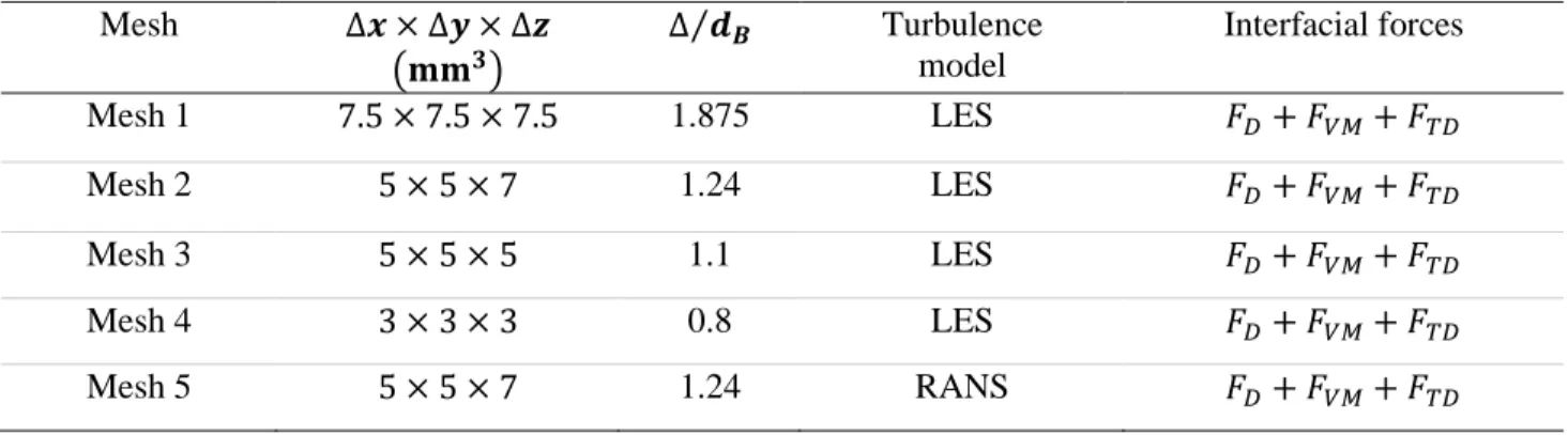
The computational mesh was generated using the Gmsh finite element mesh generator. In order to check that the computed results are grid-independent, two different grids with 𝑑𝐵⁄ 0.75, 1.1, 1.4 ∆ and 1.875 have been analysed by increasing the number of computational cells in the center of the column and the axial direction from 4 mm to 5 mm and stretching the mesh near the walls, see table
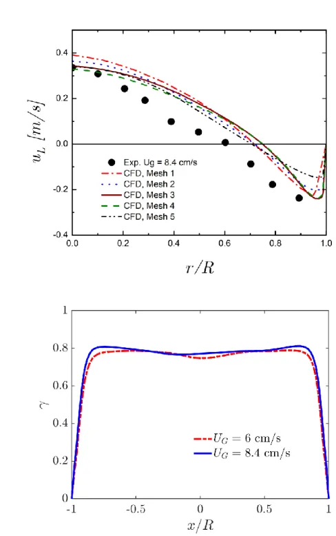
2. Milelli et al. (2001) established the criterion of the ratio of the bubble diameter to cut-off filter size: ∆ 𝑑⁄ 𝐵 ≥ 1.5, that is the mesh size must be at least 50% larger than the bubble diameter for Eulerian-Eulerian simulations. Fig. 1 shows a comparison of the axial liquid velocity and the gas hold-up. All the meshes show very similar results and mesh 3 and 4 perform better in the near-wall region. In this work, we have employed a medium mesh with a filter width ∆ = 5 mm (∆ 𝑑⁄ 𝐵= 1.1), which
quantitively seems to give better agreements and ensures a good compromise between the CPU time and accuracy at the column center and close near the walls. As you can see from Fig. 1, we have checked the non-dimensional spacing x+, y+, and z+ desirable to make a large eddy simulation setup convincing. Note that for comparison, Niceno et al. (2008) used the criterion ∆ 𝑑⁄ 𝐵= 1.2 and found no significant different with the coarser one satisfying Milelli condition, Dhotre et al. (2008) found good agreement with experimental data using both conditions ∆ 𝑑⁄ 𝐵 = 1.2 and ∆ 𝑑⁄ 𝐵= 2.5, and Liu et al. 2018 used the criterion ∆ 𝑑⁄ 𝐵≤ 1.0 and concluded that the grid size doesn’t have to be larger than a single bubble. All transient calculations are started from static conditions with the liquid at rest and the gas is injected with a mass flow rate corresponding to the experimental superficial gas velocity. We start calculations with a fixed small-time step of ∆𝑡 = 0.0005 s for the first 20 s then we increase it to 0.001 s to account for the transient instabilities of bubbly turbulent flows. The flow was simulated for 200 s and the averaged results from t = 50 s to t = 200 s are quantitively compared with experimental data. All the simulations were performed in parallel mode on a PC cluster with 16 nodes, Intel Xeon, 2.8 GHz, 4GH RAM. The different time-averaged profiles displayed in section 3 are given at the mid height of the bubble column (𝐻 = 1 m).
3. Numerical results
The resolved axial liquid velocity is presented in Fig. 1a, it can be seen that there is no significant change in the prediction between the medium and the fine mesh. In order to understand that how the LES model resolves well the fluid flow in the column numerically, Pope (2011) suggested to measure and check when the ratio of resolved kinetic energy to the total turbulent kinetic energy is greater than 80%, i.e.,
This ratio is plotted in Fig.1b at height ℎ = 0.7 m. We get the same results for different height positions in a plane normal to the axial flow direction. The ratio is around 80% with the medium grid used and the LES resolves more flow in the core regions. Hence, the resolution of the LES with the present mesh can be considered acceptable for analysis.
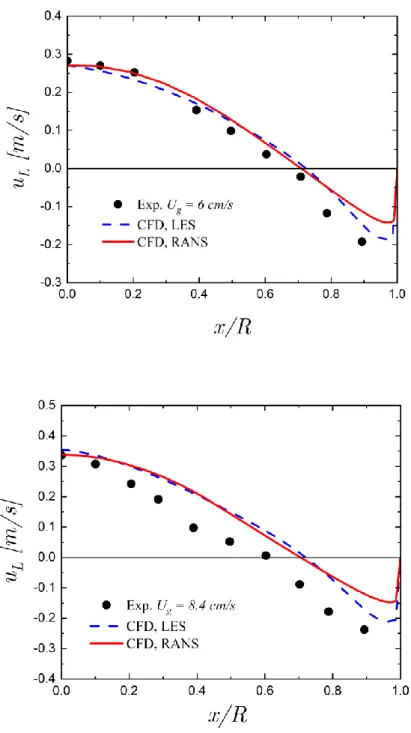
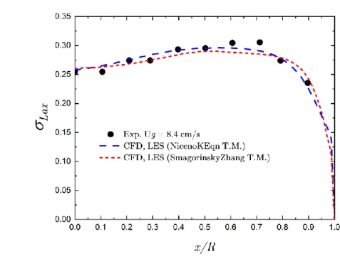
The axial liquid velocity profiles predicted by the mixture 𝑘 − 𝜀 model (Behzadi et al., 2004) and the one-equation SGS have been compared with experiments, so as to realize the relative behaviour of different turbulence models, and results are shown in Fig. 2 and 3. It can be seen that both models provide good agreements with experiments and the RANS model over predicts the liquid velocity for the near-wall region. The reason for this over estimation may come from the fact that a bubble plume moves upward in a spiral rotating manner in the center with the liquid flow meantime small spherical bubbles spirally move downward close near to the wall column accelerating the water flow and the mixture 𝑘 − 𝜀 model do not analyse this flow near the wall as well as the inappropriateness of standard wall functions developed basically for single phase flow. The one-equation SGS model predicts the overall behaviour of the axial liquid velocity profile better than the RANS model and gives good agreement with experimental measurement. For the gas hold-up the two turbulence models capture the experimental profiles reasonably well. It can be however observed that the LES model under predicts the gas hold-up at the center of the column for
−0.5 ≤ 𝑥 𝑅
⁄ ≤ 0.5
, where the flow is dominated by large-scale structures, whereas the RANS model performs much better. In the near wall region where the flow is dominated by small-scale structures, the situation is different, and the amount𝛾 = 𝑘𝑟𝑒𝑠 𝑘𝑆𝐺𝑆+ 𝑘𝑟𝑒𝑠 > 0.8, 𝑘𝑟𝑒𝑠= 1 2𝑢𝐿 ′𝑢 𝐿′ ̅̅̅̅̅̅ (15)
of the gas predicted by LES is much closer to the experimental data. The inclusion of the turbulent dispersion force in the RANS model decreases the axial liquid velocity in the core region and results in a comparatively flatter gas hold-up profile, which can predict the profile closer to the experimental data in the core region. Similar RANS results were reported by Tabib et al. (2008).
The Fig. 4 displays radial distribution of the time-averaged axial bubble velocity at the mid height of the bubble column (𝐻 = 1 m). Unfortunately, experimental measurements are not available for comparison. The results show similar trends as those reported in (Zhang et al., 2006 and Dhotre et al., 2008); the bubble plume spreading in the center and a relatively steep gas velocity profile for high superficial gas velocity which leads to less dispersed bubble plume.
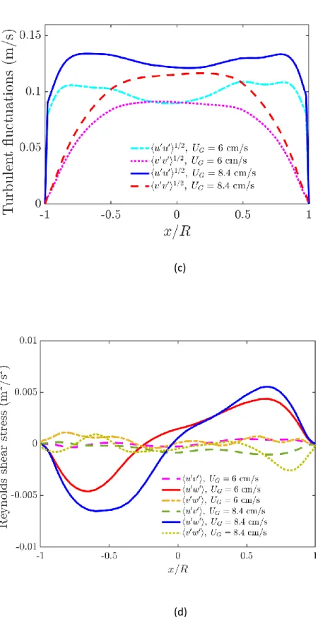
Fig. 5 shows profiles of the fluctuations of the liquid velocity at height 0.7 m. All the profiles are based on the resolved part of liquid velocities. Unfortunately, experimental data on kinetic turbulent energy of the liquid phase are not available. In fact, Vial et al. 2001 only measured the rms in the axial and orthoradial directions. In Fig. 5(b) we present a comparison of liquid fluctuations in the other directions. Clearly, the velocity fluctuations in the present bubble column reactor are anisotropic. The time-averaged spanwise component 〈𝑣′𝑣′〉1 2⁄ increases smoothly away from the wall and attains a maximum at the center of the column, whereas the streamwise fluctuations 〈𝑢′𝑢′〉1 2⁄ display a periodic trend with a lower value in the core region and attains its highest value close near to the wall in a similar way to the axial fluctuations displayed in Fig. 5(a). This is probably due to the liquid movements from upward to downward and laterally at the center and close to the wall column in which 〈𝑢′𝑢′〉 peaks with high magnitude near the wall. Ma et al. (2016) observed the same trend in their quasi-2D bubble column and Deen et al. (2001) in a 3D bubble column reactor with a non-uniform aeration faced the same scenario. As shown, the high inlet gas flow rate induces substantial turbulence both in the core and in the wall regions which changes the trend of liquid fluctuations. Furthermore, it is worth noting that values of axial liquid fluctuations are higher than the other components and dominate in both the core region and near the walls.
The liquid Reynolds shear stresses 〈𝑢′𝑣′〉 and 〈𝑣′𝑤′〉 are very small than the normal stresses and
increase with the gas flow rate as shown in Fig. 5 (c). As mentioned in Mudde et al. 1997, the large vortical flow structures significantly influence the Reynolds stresses since the vortices span the entire width of the column. Large contribution to the Reynolds shear stresses become larger in the vortical flow region since the fluctuation in the vertical component dominates close to the center region of the column where the liquid moves in a wavy manner, whereas 〈𝑢′𝑣′〉 peaks in the central plume and in the near wall region. The Reynolds shear stresses experience fluctuations due to the swinging motion of the bubble plume. At higher superficial gas velocity 𝑈𝐺 = 8.4 cm/s the intensity of the large-scale turbulence is much higher due to the bubble motion which accelerates the liquid flow and cause an overestimation of the liquid velocity in the central plume region.
Fig. 5(a) shows comparisons between experiments and numerically predicted vertical liquid velocity fluctuations where it can be seen that the one-equation SGS model can reproduce the experimental data much better than the RANS model. The time-averaged axial liquid velocities averaged through the cross-sectional area normal to the axial direction at height ℎ = 0.7 m is given in Table 3. One can see the good agreement for both gas flow rates. The effect of the turbulent dispersion was added by incorporating the sub-grid scale turbulent dispersion turbulent dispersion force using the SGS kinetic energy obtained from the one-equation LES model using mesh sizes coarser larger than the bubble size (4.5 mm). The axial liquid velocity profiles are practically the same near the wall and agree best with experimental data as we increase 𝐶𝑇𝐷. With coefficients (𝐶𝑇𝐷) larger than 0.6 the profiles don’t improve. We found that such interfacial force improves the liquid velocity profile as in Tabib et al. (2011) who have shown that even a small magnitude of turbulent dispersion SGS is enough to affect the flow profile.
Fig. 6 shows a comparison between the Smagorinsky and one-equation SGS models for the axial liquid velocity at 𝑈𝐺 = 8.4 cm/s. The resolved part by the one-equation model shows better agreement for the liquid velocity, whereas the Smaroginsky model over-predicts the experimental
data in the center and captures the trend of the down-flow circulation in the near-wall region. However, the gas hold-up is under-estimated and becomes flatter in the core region. Zhang et al. (2006) and Dhorte et al. (2008) compared different LES models. Their results over-predicted experimental profiles and become steeper for high values of 𝐶𝑆 than 0.15 since the turbulent viscosity increases and damps the bubble plume. With 𝐶𝑆= 0.08 the CFD model provides a good solution for the time-averaged axial liquid velocity. The axial liquid velocity fluctuations predicted by both models are very similar to each other. For the rest of this work we use the one-equation model to analyse the instantaneous flow as well as the energy spectra.
3.2. Instantaneous flow
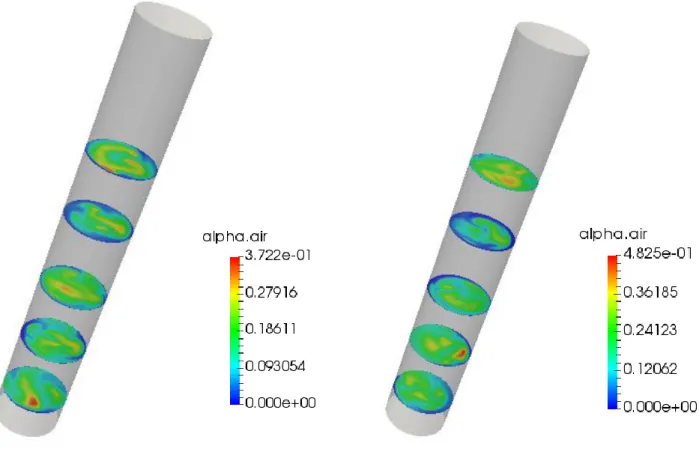
The instantaneous flow structure in 3D bubble columns was classified, based on visual study of (Chen et al., 1994; Lin et al., 1996), into four distinct regions: an oscillating plume accompanied with two staggered rows of vortices, fast bubble region, vortical flow region, and descending flow region close near the walls. A two-phase flow computational model has to capture all these features observed in the experiments. Snapshots of instantaneous liquid velocities vector field together with the gas hold-up contour plot are shown in Fig. 6 and 7 for the simulations using RANS and LES models in the plane of symmetry and several cross-sections at different superficial gas velocities. The time averaged results are also displayed in Fig. 6. The gas injected from the bottom forms clusters of bubbles that move upward in a wavy manner along the region of the central plume. Multiple smaller and larger vortex cells are continuously generated in the vortical-spiral region and along the side of the bubble plume, which stagger on each other and change their size and position in time. The behaviour of the bubble plume and the undulation shape of the bubble swarm simulated by LES are more dynamic than those obtained by RANS at the recorded instant, exhibiting more appreciable swinging motion and result in more complicated bubble-induced flow structures. The transient liquid field seems to be more uniform near the free surface at 𝑈𝐺= 6 cm/s for RANS, as a result, we see recirculating zones that push bubbles to disappear from the liquid phase. From the present LES, the
time-averaged global gas hold-up from the injector to the free-surface is found to be nearly 20%. In the cross-section the flow moves in a spiral way forth and back. In the core region, higher values of the gas hold-up are obtained meaning the existence of the central bubble region. Both the instantaneous and time-averaged snapshot show the vortical-spiral flow region close to the wall. The instantaneous profile shows that the Euler LES model has been able to capture the four flow regions and can be used to educe coherent flow structures.
There are many vorticity criteria used to identify and visualize vorticity regions and characteristic three-dimensional eddy structures, for instance, the 𝑄 − criterion, 𝜆2 − criterion, and Δ − criterion, see (Chen et al., 2015). In this work, we chose 𝜆 − 2 method to visualize the iso-surface of vortical structures coloured by the vertical liquid velocity in the column, see Fig.8. The color shows the magnitude of the liquid axial velocity, 𝜆 − 2 = −2 , where the large-scale structures consist mainly of plume structures meandering and oscillating. Complex vortical rings are formed in the central plume and vortical regions, adjacent to the descending flow region, where high velocity and velocity fluctuations are noticed, so the liquid particles tend to spin around itself forming vortices. There are more vortex loops near the sparger and at 𝑈𝐺 = 8.4 cm/s, suggesting that more turbulence is generated. Unlike RANS, furthermore, it can be seen the high degree of randomness exhibited by LES near the center and along the sidewalls. As noticed by other authors (Hu et al., 2008) this is believed that the estimated flow behaviour based on LES model, is to be closer to the real flow situation and LES resolves many more transient details of the flow, see also Fig. 1 and 2.
Overall, the instantaneous results and the liquid velocity fluctuations profiles reveal the generation of large-scale structures moving upward in meandering way in the bubble plume region and spiralling downward in the near-wall region, as shown in Fig. 6 and 7, by the formation and motion of cluster of bubbles and the subsequent bubble wake interaction. Strong vortices of different sizes are developed in the plume edge. The turbulence is anisotropic, and the liquid axial fluctuations are significantly larger than in the streamwise or spanwise directions dominating the turbulent kinetic
energy. The one-equation SGS model predicts accurately the axial liquid fluctuations and fails to capture the gas hold-up in the core plume region.
3.3. Energy spectra
Fig. 9 and 11 show a 200 s time history plot of the resolved axial and streamwise liquid velocity at one point (𝑥 𝑅⁄ = 𝑦 𝑅⁄ = 0 m, 𝑧 = 0.7 m) in the column corresponding to nearly 20,000 sample points. The transient behaviour is well reflected in the high-frequency oscillations of liquid velocities components around time averaged values, depicted in red lines, due to the turbulent fluctuations. The amplitude of fluctuations increases with the inlet gas flow rate where axial component contains more frequencies.
The energy spectrum densities (PSD) obtained from LES with data extracted from Fig. 9 and 11 and cover the time from 50 s to 200 s are shown in Fig. 10 and 12. As can be seen the spectrum displays a broad range of frequencies with slopes of about -5/3 in the frequency region between 1 and 10 Hz. For high frequency region (> 10 Hz) the decay becomes faster with a slope steeper than -3 power law. Several authors have analysed the power spectrum based on Euler-Euler LES results and obtained different slope decay in the inertial subrange region. For instance, Dhotre et al. (2008) and Ma et al. (2015) used the BIT model of Sato et al. (1981) and the obtained slope was partly over than -10/3, while Lin et al. 2018 obtained a -25/3 power laws. By comparing both predicted spectra for higher frequencies, large inlet gas flow rate gives more dissipation and the bubbles alters the PSD significantly, see Fig. 10 and 12. Two lines with slopes -5/3 and -3 are shown in the figures. For initial 𝑈𝐺 = 6 cm/s, the PSD curve have a curve close to -3 for the horizontal liquid velocity and close to – 1/3 for the axial liquid velocity, whereas for 𝑈𝐺= 8.4 cm/s the curve clearly follows the 𝑘−3 line in the high frequency inertial and dissipation region as observed experimentally in grid turbulence configurations in (Lance and Bataille, 1991; Riboux et al., 2010; Martinez Mercado et al., 2010; Prakash et al., 2016). The PSD of the spanwise velocity component, not presented here, exhibits the same behaviour for both superficial gas velocities.
Several works investigated the fast decay in the dissipation range of the spectrum and attributed it to buoyancy-generated inertia force and bubble-induced viscosity effects. Ma et al. (2015) compared their LES energy spectrum with the experimental spectrum of Akbar et al. (2012) and found that their resolved and reliable angular bubble frequencies are far away, and the frequency information related to the bubble wake is lost. The origin of the -3 slope was explained by Prakash et al. (2016), wherein the authors examined a frequency that is representative of the bubbles − 𝑓𝐵≈ |𝐔𝑟| (2𝜋𝑑⁄ 𝐵)− and it is impact on the resulting spectra. In the present case, the bubble frequency may be estimated as: 𝑓𝐵 ≈ 9 Hz, where |𝐔𝑟| ≈ 25 cm s⁄ being the bubble velocity and 𝑑𝐵= 0.0045 m the averaged bubble diameter, so that below this above the PSD changes the characteristic slope -5/3 to -3, which implies that there an energy input on the scale of bubble diameter (𝑑𝐵) and frequency of bubble motion.
4. Conclusions
Euler-Euler large eddy simulations of dispersed turbulent gas-liquid flow in a three-dimensional cylindrical bubble column, with high aspect ratio (𝐻 𝐷⁄ ) of 20 and multiple orifice gas nozzle, have been presented. Effects of all drag forces, non-drag forces, sub-grid turbulent dispersion and bubble induced turbulence are all accounted for. For the time-averaged axial liquid velocity and gas hold-up, it is found that the present model based on the one-equation SGS shows good agreement with experimental measurement data from Vial et al. 2000, and improves the axial liquid velocity of the mixture 𝑘 − 𝜀 model in the near wall regions and the bubble plume but small discrepancies in the gas hold-up were observed in the core region. The mixture 𝑘 − 𝜀 model accurately predicts the radial distribution of the gas hold-up. The flow calculated by the Euler-Euler LES model is more dynamic and more details of the instantaneous local flow structure have been obtained including large-scale structures and vortices developed in the bubble plume edge. The one-equation model performs much
better than the Smagorinsky model with 𝐶𝑆= 0.08 in the central plume and vortical flow regions. The Smagorinsky model improves the resolved axial liquid velocity profile in the near-wall region.
The effect of inlet superficial gas velocities was investigated. Two inlet superficial gas velocities, corresponding to transient and turbulent flow regimes, were chosen for simulations. It is found that the present model agrees well with experimental data for 𝑈𝐺 = 6 cm/s and small discrepancies are obtained for 𝑈𝐺 = 8.4 cm/s. The classical -5/3 law of power spectral density of the resolved liquid velocities is obtained for low frequency regions and -10/3 (-3) for high frequencies at 𝑈𝐺 = 6 cm/s (𝑈𝐺 = 8.4 cm/s). The normal Reynolds stress of the resolved part gives very good agreement with experiment and the shear stresses 〈𝑢′𝑤′〉 are similar to those obtained by Ma et al. 2015(a) using a flat rectangular bubble column reactor. The present study indicated that a CFD model based on Euler-Euler One-equation SGS LES reasonably predicted the hydrodynamics of two-phase flow in bubble column reactors in turbulent-churn flow regime.
Acknowledgements
This study was financially supported by the Spanish Ministry of Economy, Industry and Competitiveness – Research National Agency under project DPI2016-75791-C2-1-P, FEDER funds and by Generalitat de Catalunya – AGAUR under project 2017 SGR 01234.
References
1
Behzadi, A., Issa, R. I., Rusche, H., 2004. Modelling of dispersed bubble and droplet flow at high phase fractions, Chem. Eng. Sci. 59, 759-770.2
Bove, S., Solbergt, T., Hjertager, B. H., 2004. Numerical aspects of bubble column simulations, Int. J. Chem. Reactor Eng. 2, 1-22.3
Chen, R.C., Reese, J., Fan, L.-S., 1994. Flow structure in a three-dimensional bubble columns and three-phase fluidized bed. AIChE J. 40, 1093-1104.4
Chen, Q., Zhong, Q., Qi., M., Wang, X., 2015. Comparison of vortex identification criteria for planar velocity fields in wall turbulence. Phys. Fluids 27 (8) 2015.5
Darmana, D., Deen, N. G., Kuipers, J. A. M., Harteveld, W. K., Mudde, R. F., 2009. Numerical study of homogeneous bubbly flow: influence of the inlet conditions to the hydrodynamic behaviour, Int. J. Multi. Flow 35, 1077-1099.6
Davidson, L., 1997. Large-eddy simulations: a note on derivation of the equations of the subgrid turbulent kinetic energies. Technical Report No. 97/12, 980904, Chalmers University of Technology, Gothenburg, Sweden.7
Deen, N. G., Hjertager, B. H., Solberg, B. H., 2001. Large eddy simulation of the gas-liquid flow in a square cross-sectioned bubble column, Chem. Eng. Sci. 56, 6341-6349.8
Dhotre, M. T., Niceno, B., Smith, B. L., 2008. Large eddy simulation of a bubble column using dynamic sub-grid scale model, Chem. Eng. J. 136, 337-348.9
Dhotre, M. T., Niceno, B., Smith, B. L., Simiano, M., 2009. Large eddy simulation (LES) of large-scale bubble plume, Chem. Eng. J. 64, 2692-2704.10
Dhotre, M. T., Deen, N. G., Niceno, B., Khan, Z., Joshi, J. B., 2013. Large eddy simulation for dispersed bubbly flows: A review, Int. J. Chem. Eng. Vol. 2013, ID 343276, 22 pages.11
Ekambara, K., Dhotre, M. T., 2010. CFD simulation of bubble column, Nuc. Eng. Des. 240, 963-969.12
Huang, Z., McClure, D. D., Barton, G. W., Fletcher, D. F., Kavanagh, J. M., 2018. Assessment of the impact of the bubble size modelling in CFD simulations of alternative bubble column configurations operating in the heterogenous regime, Chem. Eng. Sci. 186, 88-111.13
Hu, G., Celik, I., 2008. Eulerian-Lagrangian based large-eddy-simulation of a partially aerated flat bubble column, Chem. Eng. Sci. 63, 253-271.14
Ishii, M., Hibiki, T., 2006. Thermo-fluid dynamics of two-phase flow, 2nd edition, Springer, New York.15
Joshi, J. B., 2001. Computational flow modelling and design of bubble column reactors, Chem. Eng. Sci. 56, 5893-5933.16
Khan, Z., Mathpati, C. S., Joshi, J. B., 2017. Comparison of turbulence models and dynamics of turbulence structures in bubble column reactors: effects of sparger design and superficial gas velocities, Chem. Eng. Sci. 164, 34-52.17
Kouzbour, S., Stiriba, Y., Gourich, B., Vial, Ch., 2020. CFD simulation and analysis of reactive flow for dissolved manganese removal from drinking water by aeration process using an airlift reactor, J. Water Proc. Eng. 36, 101352.18
Krishna, R., van batten, J.M., 2001, Eulerian simulations of bubble columns operating at elevated pressures in the churn turbulent flow regime, Chem. Eng. Sci. 56, 6249-6258.19
Lin, T.-J., Reese, J., Hong, T., Fan, L.-S., 1996. Quantitative analysis and computation of two-dimensional bubble columns. AIChE J. 42, 301-318.20
Liu, Z., Li, B., 2018. Scale-adaptive analysis of Euler-Euler large eddy simulation for laboratory scale dispersed bubbly flows, Chem. Eng. J. 338, 465-477.21
Lopez de Bertodano, M., Lahey Jr, R., Jones, O., 1994. Phase distribution in bubbly two-phase flow in vertical ducts, Int. J. Multiph. Flow 20 (5), 805-818.22
Lu, J., Tryggvason, G., 2013. Dynamics of nearly spherical bubbles in a turbulent channel upflow, J. Fluid Mechanics 732, 166-189.23
Ma, T., Ziegenhein, T., Lucas, D., Frohlich, J., 2015a. Large-eddy simulations of the gas-liquid flow in a rectangular bubble column, Nuc. Eng. Des. 299, 146-153.24
Ma, T., Ziegenhein, T., Lucas, D., Frohlich, J., 2015b. Euler-Euler large-eddy simulations for dispersed turbulent bubbly flows, Int. J. Heat Fluid Flow 299, 146-153.25
Martínez Mercado, J., Chehata, D., van Gils, D.P.M., Sun, C., Lohse, D., 2010. On bubble clustering and energy spectra in pseudo-turbulence, J. Fluid. Mech. 650, 287-306.26
Niceno, B., Dhorte, M. T., Deen, N. G., 2011. One-equation sub-grid (SGS) modelling for Euler-Euler large eddy simulation (EELES) of dispersed bubbly flow, Chem. Eng. Sci. 63 (15), 3923-3931.27
Olmos, E., Gentric, C., Vial, Ch., Wild, G., Midoux, N., 2001. Numerical simulation of multiphase flow in bubble column reactors. Influence of bubble coalescence and break-up, Chem. Eng. Sc. 56, 6389-6365.28
Olmos, E., Gentric, C., Vial, Ch., Midoux, N., 2003. Identification of flow regimes in a flat gas-liquid bubble column via Wavelet transform, Can. J. Chem. Eng. 81, 382-388.29
OpenFOAM Ltd., United Kingdom, 2012, OpenFOAM 2.1.1 user’s guide.30
Prakash, V.N., Mercado, J.M., van Wijngaarden, L., Mancilla, E., Tagawa, Y., Lohse, D., Sun, C., 2016. Energy spectra in turbulent bubbly flows, J. Fluid. Mech. 791, 174-190.31
Pope, S., Turbulent flows, 2011. Cambridge University Press.32
Riboux, G., Risso, F., Legendre, D., 2010. Experimental characterization of the agitation generated by bubbles rising at high Reynolds number, J. Fluid. Mech. 643, 509-539.33
Rusche, H., 2002. Computational fluid dynamics of dispersed two-phase flows at high phase fractions. Ph.D. Thesis, Imperial College, University of London.34
Sato, Y., Sekoguchi, K., 1975. Liquid velocity distribution in two-phase bubbly flow. Int. J. Multiphase Flow 2, 79-95.35
Sokolichin, A., Eigenberger, G., 1999. Applicability of the standard k-ε turbulence model to the dynamic simulation of bubble columns: Part 1. Detailed numerical simulations, Chem. Eng. Sci. 54, 2273–2284.36
Sokolichin, A., Eigenberger, G., Lapin, A., 2004. Simulation of buoyancy driven bubbly flow: Established simplifications and open questions, AIChE J. 50, 24–45.37
Y. Stiriba, B. Gourich, Ch. Vial, 2017. Numerical modelling of ferrous iron oxidation in a split-rectangular airlift reactor, Chem. Eng. Sci., 170, 705-719.38
Tabib, M. V., Schwarz, P., 2008. CFD simulation of bubble column – an analysis of interphase forces and turbulence models, Chem. Eng. Sci. 139, 589-614.39
Tabib, M. V., Schwarz, P., 2011. Quantifying sub-grid (SGS) turbulent dispersion force and its effect using one-equation SGS large eddy simulation (LES) model in a gas-liquid and a liquid-liquid system, Chem. Eng. Sci. 68, 3071-3086.40
Tomiyama, A., Tamai, H., Zun, I., Hosokawa, S., 2002. Transverse migration of single bubbles in simple shear flows, Chem. Eng. Sci. 57, 1849-1858.41
van der Hengel, E. I. V., Deen, N. G., Kuipers, J. A. M., 2005. Application of coalescence and breakup models in a discrete bubble model for bubble column, Ind. Eng. Chem. Research 44, 5233-5245.42
Vial, Ch., Camarasa, E., Poncin, S., Wild, G., Midoux, N., Bouillard, J., 2000. Influence of gas distribution and regime transition on liquid velocity and turbulence in a bubble column, Chem. Eng. Sci. 55, 2957-2973.43
Vial, Ch., Lainé, R., Poncin, S., Midoux, N., Wild, G., 2001. Influence of gas distribution and regime transition on liquid velocity and turbulence in a bubble column, Chem. Eng. Sci. 56, 1085-1093.44
Vial, Ch., Stiriba, Y., 2013. Characterization of bioreactors using computational fluid dynamics, Fermentation Processes Engineering in the Food Industry, C.R. Soccol, A. Pandey, C. Larroche Eds. – Taylor & Francis Group – 978-1-4398-8765-3, 121–164.45
Weller, H. G., Tabor, G., Jasak, H., Fureby, D., 1998. A tensorial approach to computational continuum mechanics using object-oriented techniques, Comput. Phys. 12, 620-631.46
Zhang, D., Deen, N. G., Kuipers, H. A. M., 2008. Numerical simulation of the dynamic flowbehavior in a bubble column: A study of closures for turbulence and interface forces, Chem.
Eng. Sci. 61, 7593-7608.
47
Ziegenhein, T., Rzehak, R., Ma, T., Lucas, D., 2017. Towards a unified approach for modelling uniform and non-uniform bubbly flows, Canadian J. Chem. Eng. 95, 170-179.Reference Bubble column dimensions
Gas distributor Bubble diameter
Superficial gas velocity
SGS model
Deen et al., 2001 Rectangular column, 𝑊 = 0.15 m, 𝐷 = 0.15 m, 𝐻 = 1 m Perforated plate, 49 holes of 𝐷 = 1 mm 4 mm 0.49 cm/s Smagorinsky, 𝐶𝑆= 0.1 Bove et al., 2004 Rectangular column,
𝑊 = 0.05 m, 𝐷 = 0.2 m, 𝐻 = 0.45 m Perforated plate, 49 holes of 𝐷 = 1 mm 4 mm 0.5 cm/s VLES, 𝐶𝑆= 0.12 van den Hengel
et al., 2005 Zhang et al., 2006 Rectangular column, 𝑊 = 0.15 m, 𝐷 = 0.15 m, 𝐻 = 1 m Rectangular column, 𝑊 = 0.15 m, 𝐷 = 0.15 m, 𝐻 = 1 m Perforated plate, 49 holes of 𝐷 = 1 mm Perforated plate, 49 holes of 𝐷 = 1 mm 3 mm 4 mm 0.5 cm/s 0.49 cm/s Smagorinsky with DBM Smagorinsky, 𝐶𝑆= 0.08 − 0.2 Niceno et al., 2008 Rectangular column, 𝑊 = 0.15 m, 𝐷 = 0.15 m, 𝐻 = 1 m Perforated plate, 49 holes of 𝐷 = 1 mm 4 mm 0.5 cm/s One-equation SGS Dhotre et al., 2008 Rectangular column, 𝑊 = 0.15 m, 𝐷 = 0.15 m, 𝐻 = 1 m Perforated plate, 49 holes of 𝐷 = 1 mm 4 mm 0.5 cm/s Smagorinsky 𝐶𝑆= 0.12, and dynamic Smagorinsky Hu and Celik, 2008 Rectangular column, 𝑊 = 0.08 m, 𝐷 = 0.15 m, 𝐻 = 2 m
Flush mounted, 5 porous dicks of 𝐷 = 40 mm 1.6 mm 0.66 cm/s Smagorinsky, 𝐶𝑆= 0.032 Darmana et al., 2009 Ekambara et al. 2010 Tabib and Schwarz, 2011 Ma et al., 2015 Ma et al., 2016 Khan et al., 2017 Rectangular column, 𝑊 = 0.24 m, 𝐷 = 0.072 m, 𝐻 = 0.8 m Cylindrical column, 𝐷 = 0.15 m, 𝐻 = 0.9 m Cylindrical column, 𝐷 = 0.15 m, 𝐻 = 1 m Rectangular column, 𝑊 = 0.243 m, 𝐷 = 0.04 m, 𝐻 = 1 m Rectangular column, 𝑊 = 0.2 m, 𝐷 = 0.05 m, 𝐻 = 0.45 m Cylindrical column, 𝐷 = 0.15 m, 𝐻 = 1 m
Multiple gas injection of 95 needles of 𝐷 = 0.51 mm Multipoint perforated plate, 25 holes of 𝐷 = 2 mm Multipoint perforated plate, 25 holes of 𝐷 = 2 mm
Multiple gas injection of 35 needles Set of 8 holes in a rectangular configuration: 0.02 m × 0.0125 m Multipoint perforated plate, 25 holes of 𝐷 = 2 mm 4 mm 6 mm 3-5 mm iMUSIG, 2 groups 2 mm 5 mm 0.7 cm/s 0.2 cm/s 2 cm/s 0.3 and 1.3 cm/s 0.17 cm/s 2 – 10 cm/s SGS of Vreman , 𝐶𝑆= 0.1 Smagorinsky, 𝐶𝑆= 0.12 One-equation SGS Smagorinsky, 𝐶𝑆= 0.15 Dynamic Smagorinsky Smagorinsky, 𝐶𝑆= 0.5 Liu and Li, 2018 Rectangular column,
𝑊 = 0.15 m, 𝐷 = 0.15 m, 𝐻 = 1 m
Perforated plate, 49 holes of 𝐷 = 1 mm
4 mm 0.5 cm/s Dynamic Smagorinsky
Present work Cylindrical column, 𝐷 = 0.1 m, 𝐻 = 2 m
Multiple orifice plate, 62 orifices of 𝐷 = 1 mm 4.5 mm 6 and 8.4 cm/s Smagorinsky with 𝐶𝑆= 0.08, and one-equation SGS
Mesh ∆𝒙 × ∆𝒚 × ∆𝒛 (𝐦𝐦𝟑) ∆ 𝒅⁄ 𝑩 Turbulence model Interfacial forces Mesh 1 7.5 × 7.5 × 7.5 1.875 LES 𝐹𝐷+ 𝐹𝑉𝑀+ 𝐹𝑇𝐷 Mesh 2 5 × 5 × 7 1.24 LES 𝐹𝐷+ 𝐹𝑉𝑀+ 𝐹𝑇𝐷 Mesh 3 5 × 5 × 5 1.1 LES 𝐹𝐷+ 𝐹𝑉𝑀+ 𝐹𝑇𝐷 Mesh 4 3 × 3 × 3 0.8 LES 𝐹𝐷+ 𝐹𝑉𝑀+ 𝐹𝑇𝐷 Mesh 5 5 × 5 × 7 1.24 RANS 𝐹𝐷+ 𝐹𝑉𝑀+ 𝐹𝑇𝐷
Superficial gas velocity (cm/s) 6 8.4
Experimental (m/s) 0.2 0.25
CFD (m/s) 0.211 0.257
Table 3. Experimental and numerical centerline axial fluctuations of the liquid velocity Table 2. The computational mesh and grid spacing investigated
Fig. 1 Mesh independence analysis; comparison of the time-averaged results for the axial liquid and the different meshes investigated at 𝑈𝐺 = 8.4 cm/s (top); the ratio, 𝛾, resolved kinetic energy to total kinetic energy (bottom).
Fig. 2 Comparison between the simulated and experimental profiles of the axial liquid velocity at superficial gas velocity 𝑈𝐺 = 6 cm/s (top) and 𝑈𝐺 = 8.4 cm/s (bottom).
Fig. 3 Comparison between the simulated and experimental profiles of the gas hold-up at superficial gas velocity 𝑈𝐺 = 6 cm/s (top) and 𝑈𝐺= 8.4 cm/s (bottom).
Fig. 4 Time averaged axial gas velocity at superficial gas velocity 𝑈𝐺 = 6 cm/s and 𝑈𝐺 =
(a)
Fig. 5 Comparison between the simulated and experimental profiles of the axial rms liquid velocity fluctuations (a) and (b), turbulent fluctuations (c), and Reynolds shear stress (d).
(c)
Fig. 6 Comparison between the simulated axial liquid velocity (top), the gas hold-up (center) and rms axial liquid velocity fluctuation results obtained using Smagorinsky and one-equation SGS models (bottom).
Fig. 7 Snapshots of instantaneous gas hold-up and liquid velocity field with RANS model (left) and LES model (center) and time averaged LES (right) at 𝑈𝐺 = 6 cm/s (top), and 𝑈𝐺 = 8.4 cm/s
Fig. 9 Instantaneous vortical structure at time 𝑇 = 200s by 𝜆 − 2 method coloured by the magnitude of the liquid velocity, 𝜆 − 2 = −2.0; at 𝑈𝐺= 6 cm/s (left), and 𝑈𝐺= 8.4 cm/s (right).
Fig. 10 Time history of the axial liquid velocity (top) and horizontal liquid velocity (bottom) with one-equation SGS model at the centerline of the column, at a height of 𝑧 = 0.7 m and 𝑈𝐺 = 6 cm/s.
Fig. 11 Power spectrum density of horizontal liquid velocity (top) and vertical liquid velocity (bottom) at 𝑈𝐺= 6 cm/s.
Fig. 12 Time history of the axial liquid velocity (top) and horizontal liquid velocity (bottom) with one-equation SGS model at the centerline of the column, at a height of 𝑧 = 0.7 m 𝑈𝐺 = 8.4 cm/s.
Fig. 13 Power spectrum density of axial liquid velocity (top) and horizontal liquid velocity (bottom) at 𝑈𝐺 = 8.4 cm/s.
Nomenclature
𝐶𝐷 drag force coefficient 𝐶𝐿 lift force coefficient 𝐶𝑆 Smagorinsky constant
𝐶𝑇𝐷 turbulent dispersion coefficient 𝐶𝑉𝑀 virtual mass force coefficient
𝐶𝜇,𝐵𝐼 constant in bubble induced turbulence model 𝑑𝐵 bubble diameter, m
𝐷 diameter of the column, m 𝑔 gravity acceleration, m s-2 𝐻 height of the column, m
𝑘𝜑 turbulent kinetic energy of phase 𝜑, m2 s-2 𝑘𝑆𝐺𝑆 Sub-grid scale kinetic energy of phase, m2 s-2
𝐌𝜑 total interfacial force acting between the phase 𝜑 and the other phase, N m-3 𝐌𝜑𝐷 drag force for the phase 𝜑, N m-3
𝐌𝜑𝐿 lift force for the phase 𝜑, N m-3
𝐌𝜑𝑇𝐷 turbulent dispersion force for the phase 𝜑, N m-3 𝐌𝜑𝑉𝑀 virtual mass force for the phase 𝜑, N m-3
𝑝 pressure, N m-2 𝑟 radial radius, m 𝑅 column radius, m
𝑅𝑒𝐵 bubble Reynolds number
𝑡 time, s
𝐔𝜑 resolved velocity of phase 𝜑, m s-1 𝐔𝑟 relative velocity, m s-1
𝑈𝐺 superficial gas velocity, m s-1 𝑢′ fluctuating velocity, m s-1
𝑢𝐿 time-averaged axial liquid velocity, m s-1 𝑊 width of the rectangular column, m
Greek symbols
∆ grid size, m ∆𝑡 time step, s
∆𝑥 grid spacing in 𝑥 direction, m ∆y grid spacing in 𝑦 direction, m ∆z grid spacing in 𝑧 direction, m 𝛼𝜑 gas fraction of phase 𝜑
𝜈𝐿,𝐿 liquid molecular viscosity, m2 s-1 𝜈SGS sub-grid scale viscosity, m2 s-1
𝜈𝜑eff effective viscosity, m2 s-1
𝜈𝐿,Tur shear-induced turbulent viscosity, Pa s 𝜇𝐿,BIT bubble induced viscosity, Pa s
𝜌 density, kg/m3
𝜏𝜑 shear stress of phase 𝜑, Pa
Subscripts
Highlights:
• Euler-Euler Large Eddy Simulations (LES) of dispersed turbulent gas-liquid flows in a cylindrical bubble column of high-aspect ratio (𝐻 𝐷⁄ ) of 20 at high superficial gas velocity where vortical-spiral and turbulent flow regimes.
• Analysis of the performance of the one-equation SGS model.
• Investigation of the influence of superficial gas velocity using the OpenFOAM package. • Analysis of the energy spectra of the resolved liquid velocities in churn-turbulent regime.