The effect of firms reporting to the Carbon disclosure project on their CO2 emissions. : An empirical study based on the synthetic control approach

(1)

The effect of firms reporting to the Carbon

disclosure project on their

CO2 emissions

An empirical study based on the synthetic control

approach

Doctoral Thesis

Presented to the Faculty of Economics and Social Sciences at the University of Fribourg (Switzerland), in fulfilment of requirements for the degree of Doctor of Economics and Social Sciences

by

Adéla Wyncoll

from Czech Republic

Accepted by the Faculty of Economics and Social Sciences on 03.04.2017 at the proposal of

Prof. Dr. Laurent Donz´e (First supervisor) and Prof. Dr. Martin Huber (Second supervisor)

(2)

(3)

“Mojí mamince!”

Typeset with LA_TEX

(4)

(5)

List of Tables

2.1 Data set . . . 23

2.2 Control units’ weights . . . 32

2.3 Predictors’ weights . . . 32

2.4 Treatment effects . . . 32

2.5 Predictors . . . 32

2.6 Different synthetic control method results representations . . . 32

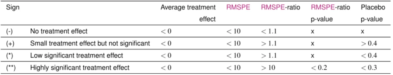
2.7 Interpretation of root mean squared prediction error measures . . . 44

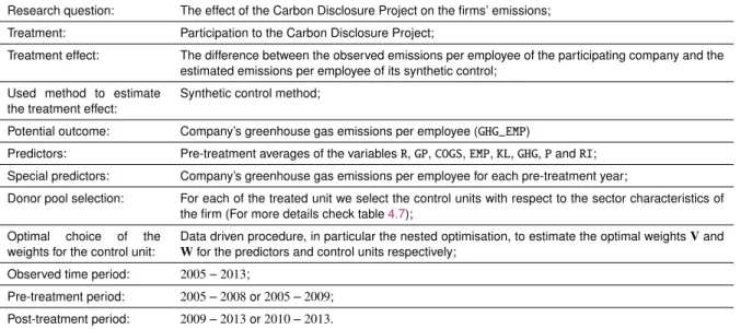
4.1 Research questions, variables and expectations . . . 71

4.2 Variables in the panel database . . . 75

4.3 Global database in numbers . . . 82

4.4 Source of the reported company’s emissions within the years . . . 83

4.5 Summary statistics (panel data on 9 years) . . . 86

4.6 Important elements of the model . . . 89

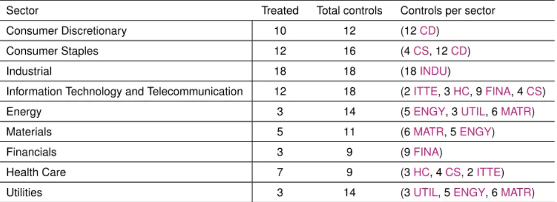
4.7 Constitution of the donor pools . . . 91

4.8 Correlations and significance of the correlations . . . 95

4.9 Functions in the package “Synth” and library “Mylib” . . . 97

5.1 Summary results . . . 102

5.2 Treatment effect signs’ explications . . . 103

5.3 Summary of significant treatment effects . . . 103

5.4 Placebo tests results . . . 104

5.5 Summary results by region . . . 105

5.6 Summary of significant treatment effects by region . . . 106

5.7 Summary results by sector . . . 108

5.8 Summary of significant treatment effects by sector . . . 109

A.1 Variables in the transversal database . . . 130

A.2 Company’s names . . . 131

A.3 One observation from the data . . . 132

A.4 Descriptive statistics for different variables - Transversal database . . . 133

A.5 Cross-table country and sector for all countries . . . 134

A.6 Cross-table country and sector for participating countries . . . 135

A.7 Crosstable country and sector for non-participating countries . . . 136

A.8 Summary statistics (panel data on 9 years) sector “Consumer Discretionary” . . . . 136

A.9 Summary statistics (panel data on 9 years) sector “Consumer Staples” . . . 137

(10)

A.14 Summary statistics (panel data on 9 years) sector “Information technology and tele-comunication” . . . 139

A.15 Summary statistics (panel data on 9 years) sector “Utilities” . . . 140

(11)

List of Figures

2.1 Treatment effect . . . 24

2.2 Synthetic control matching . . . 26

2.3 Treatment effect estimation . . . 28

2.4 Different examples of path and gaps plots . . . 34

2.5 Gaps graph . . . 35

2.6 In-space placebo procedure . . . 40

2.7 Different examples of placebo effect plots . . . 41

2.8 Leave-one-out distribution of the synthetic control for the treated unit . . . 46

4.1 Graph of average statistics . . . 84

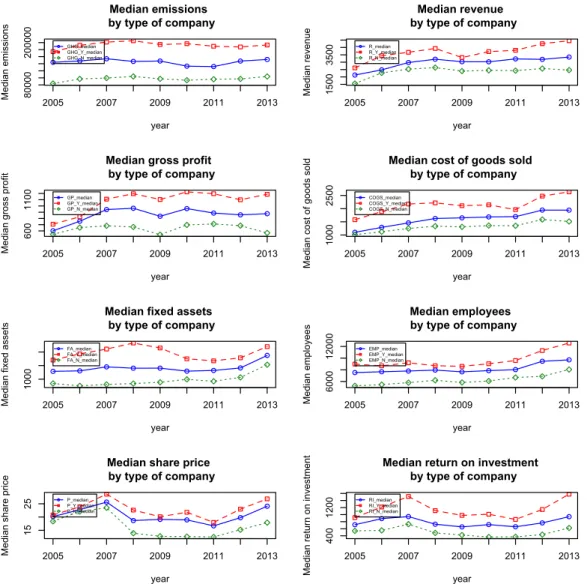
4.2 Graph of median statistics . . . 85

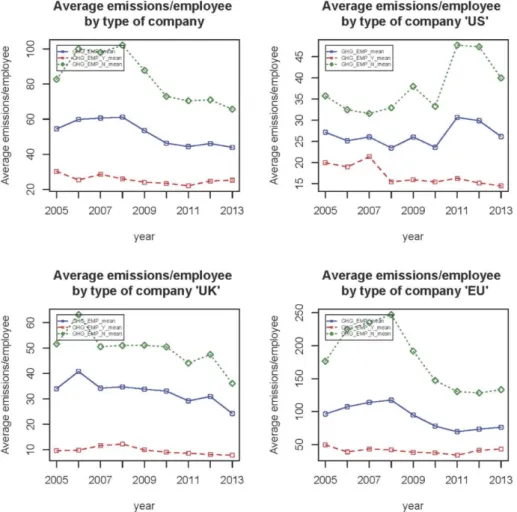
4.3 Average emissions per employee (company and regions) . . . 87

4.4 Application of synthetic control method (withTO+1 = 5) . . . 91

4.5 Functions interactions in R and steps in the job . . . 100

5.1 Synthetic matching and permutation tests for companies from information technology and telecommunications’ sector and from United States, European Union, and two from United Kingdom respectively . . . 107

5.2 Synthetic matching and permutation tests for Mcbride Plc, Constellationa, and Estee Lauder . . . 113

A.3 Results of the function synth() for company “DEBENHAMS” . . . 141

A.4 Treated effects for company “DEBENHAMS” . . . 141

A.5 Optimal weights for synthetic control of the company “DEBENHAMS” . . . 142

A.6 Predictors’ weight for synthetic control of the company “DEBENHAMS” . . . 142

A.7 Treated effects for company “DEBENHAMS” . . . 143

A.8 Path and gaps plots of the company “DEBENHAMS” . . . 144

A.9 In-space placebo treated effects, exemple of the company “DEBENHAMS” . . . 145

A.10 Root mean squared prediction errors and related statistics in-space placebo, exem-ple of the company “DEBENHAMS” . . . 146

A.11 Placebo plot of the company “DEBENHAMS” . . . 147

A.12 Placebo plots of the company “DEBENHAMS” (with different root mean squared prediction error exclusion rules) . . . 148

A.13 Synthetic matching and permutation tests Gtech, Nokian, Valeo, Greencore . . . . 150

A.14 Synthetic matching and permutation tests Jeronimo, Koninklijke, Atlantia, Centrotec 151 A.15 Synthetic matching and permutation tests Dcc, FlSmidth, Kobenhavns, Kone . . . . 152

(12)

A.20 Synthetic matching and permutation tests Pace, Savills, Leggett, Lowescos . . . 157

A.21 Synthetic matching and permutation tests VfCorp, Constallationa, EsteeLauder, Her-shey . . . 158

A.22 Synthetic matching and permutation tests Philipmorris, Abm, Actavis, Celgene . . . 159

A.23 Synthetic matching and permutation tests Akamai, Broadcom, Cognizant, Microhip 160

(13)

List of Scripts

B.1 My library . . . 164

B.2 Synthetic control analysis customer discretionary sector . . . 175

(14)

(15)

Acknowledgements

Emil Zátopek, a Czech long-distance runner, was the first and only man to win the “Triple Crown” of the 5000 metres, 10000 metres and the marathon in the Helsinki Olympic Games in 1952. His spirit was to always set new challenges, pushing himself to his limits, and hit every goal, one by one. His spirit has always inspired me along this long journey of doctoral studies. Many times I encountered obstacles holding me back, but like Emil Zátopek, I never gave up, and now I can successfully submit my thesis.

Foremost, I would like to express my sincere gratitude to my supervisor Prof. Dr. Laurent Donzé from University of Fribourg, Applied Statistics and Modelling (Department of Informatics). During the past 10 years, this person became not only my mentor but also a very good friend of mine, a person that kept a sense of humour when I had lost mine! I have to express my appreciation for the continuous support of my doctoral study and research, for his patience, and motivation. His guidance was a constant help throughout my research and writing of this thesis.

Besides my advisor, I would like to thank the rest of my thesis committee: Prof. Dr. Martin Huber, and Prof. Dr. Dirk Morschett, for their encouragement, insightful comments, and hard questions.

I also would like to thank Prof. Ralph Winkler from Bern University, Department of Economics and Oeschger Centre for Climate Change Research, for enlightening me at the first stages of research. The several meetings I had with him at the beginning of my doctoral studies helped me to connect to the idea of the evaluation of the environmental program by the synthetic control method.

My sincere thanks also go to Fredrik Fogde, Project Manager at South Pole Group, the source of a great deal of my data for my thesis, and who helped me in the process of data collection. Moreover, I could have several fruitful conversations with Frederic which helped me in terms of understanding the data and different processes concerning the reporting behaviours of the firms.

Furthermore, I must also express my very profound gratitude to my husband Stuart Wyncoll for providing me with unfailing support and continuous encouragement throughout my years of study and through the process of researching and writing this thesis. I am also indebted to my master Daisaku Ikeda, best friends Valda Hale, Marta Keane, great buddhist friends Isabelle Spuehler, Karina Arnold, my therapist/close friend Julia Rod, and colleagues/friends Redina Berkachi, and Jean-Pierre Bresciani, for hours of discussions, support and encouragements that helped me to keep my focus and head up to reach the end of my thesis.

(16)

during my process of research and writing; but also to my grandmothers Anna Divišová, and Marie Turková who always believed in me and could touch my heart with their warm encouragements.

(17)

Abstract

Whoever is not “green” is not “in”. That’s the latest trend of the market. This environmental move-ment pushes the companies to review their policies and assure a sustainable developmove-ment by reducing theirCarbon Dioxide (CO2)emissions and use of natural resources or in general show an eco-friendly behaviour.

The objective of our work is to assess the pertinence of green policy introduction at the business level. For our analysis, we are using unique data sets of the firm’s CO2emissions. We built our data by adding several firms’ characteristics to an initial database provided by South Pole Group. Based on particular companies’ specificities we were then able to select the suitable treated and control groups.

Carbon Disclosure Project (CDP)is a non-profit organisation allowing companies to report and

manage their emissions, climate risk and reduction goals. And in our study, we intend to evaluate whether signing up to theCDPhas a positive effect on the firms’ emissions.

It is a typical causal effect evaluation problem that we solve using a relatively new approach called “Synthetic Control Method (SCM)” introduced byAbadie and Gardeazabal(2003). The ob-jective of this method is to build the synthetic control unit, which is the weighted combinations of available control units that most closely resemble the treated unit before the treatment in term of different characteristics. This synthetic control unit allows us to define the counterfactual outcome, that is then compared to the actual outcome to evaluate the treatment effect. We chose the syn-thetic control method because it allows researchers to analyse phenomena that occur in a limited population or that apply to only a small number of firms, which is ideally suited to our problematic.

Almer and Winkler(2013) used this method in environmental problematic, but to our knowledge,

it has never been applied to evaluate firms’ politics, and indeed we will use this approach to analyse the environmental programme at a company level.

To complete the investigation of the general impact of this program on firms’ emissions, we also focus on three geographic regions: theUnited States (US), theUnited Kingdom (UK), and the rest

of European Union (EU). Moreover, the study also covers the comparison of results between all

sectors of activities.

(18)

(19)

Introduction

Nowadays, most of the world is aware of the irreversible climate change and the impact of this in-stance on the entire planet. As covered in the Stern Review (Stern(2006)), even the most powerful economies, who are the biggest greenhouse gas emitters, are not prevented from the effect of the raising temperature. This phenomenon increases the need of “green” and sustainable economies to mitigate the climate change and assure the future. Consequently, the companies are pushed to quickly and significantly cut down their greenhouse gas emissions and revise their actions in this direction.

Many policies, international agreements and regulations, that are also introduced in this work exist to control the greenhouse gas emissions and mitigate the climate change. The question that naturally arises is “how do we evaluate the pro-environmental behaviour?”

To answer that, numerous studies assessing the introduction of climate agreements were con-ducted on the macro scale. For example, we can cite work of Aichele and Felbermayr(2012) or

Almer and Winkler(2013), who evaluated the Kyoto Protocol. Almer and Winkler(2013) used the

synthetic control method in environmental problematic, but to our knowledge, it has not been ap-plied to assess a firm’s policy such as environmental programmes at the company level. This lack in the application of the synthetic control method catches our attention.

The primary objective of our study is to assess the pertinence of green policy introduction at the business level. More precisely, we intend to evaluate whether participating to the Carbon Disclosure Project1_{, as one of the binding reporting standards, has a positive effect on the firm’s emissions.} This is a typical causal effect problem that we solve by using a relatively new method, that is the synthetic control approach.

The synthetic control method is one of many program evaluations’ approaches that seeks the estimation of the treatment effect of particular program or treatment. Introduced by Abadie and

Gardeazabal(2003), this approach provides a data-driven procedure to estimate synthetic control

units based on a weighted combination of control units that approximates the characteristics of the unit exposed to the treatment. Moreover, with this approach, we can estimate the treatment effect in settings where a single unit is exposed to treatment, or where we dispose few historical data. We

1_CDP_{is a not-for-profit organisation that runs the global disclosure system for investors, companies, cities, states}

and regions to manage their environmental impacts. Founded in 2003 and based in the United Kingdom. Its primary goal is to help the corporations and cities to disclose the greenhouse gas emissions and assist them to manage the environmental risk.

(20)

start from the principle that a combination of comparison units often provides a better comparison for the unit exposed to the intervention than any comparison unit alone. By its characteristics, the synthetic control method allows us to generate treatment effects for each of the studied companies, and perform statistical inferences.

Furthermore, our work covers several research questions. The first general question asks if there is a positive impact of the Carbon Disclosure Project on the participating companies’ emis-sions. The second research question is focussed on the comparison of the results between three different geographic regions, which are theEU, theUK, and theUS. Note that it was the similar-ity in the economic development and the environmental strategies that lead us to the choice of these regions. Last research question inquires whether there is one of the nine sectors of activities

(Financials (FINA),Health Care (HC),Information Technology and Telecommunication (ITTE),

Con-sumer Discretionary (CD),Consumer Staples (CS),Industrials (INDU),Energy (ENGY),Materials

(MATR), Utilities (UTIL)), or any of three emitter groups (light, medium, or heavy carbon dioxide

emitters), that would be more successful in the program participation than the others.

Another objective of our work is to do a complete and detailed review of the synthetic control approach. Note that this method is covered in four papers by Abadie and al. (Abadie and

Gardeaz-abal(2003);Abadie et al.(2010,2011,2015)), where the authors assess different political problems

and develop the synthetic control method, as well as the tests used to evaluate the significance of the results. In our work, we do review all the papers and present the main elements of the method, the way of showing the results, and all different statistical inferences that the approach allows. Moreover, we also cover the application of the synthetic control method in the statistical programR

Core Team(2013) and present how we used the package “Synth” developed byHainmueller and

Diamond(2015).

An essential element to mention is the quality and uniqueness of our database. Collecting the historical data on the carbon dioxide emissions on the firm’s level is still quite a challenging task, as the companies are not usually holding the historical data. With the contribution of the South Pole Group, we were able to collect the data for a total of139companies between the years2005

to2013. This data contains carbon dioxide emissions and other characteristics of the firms that do or do not participate in the Carbon Disclosure Project. Moreover, the data covers nine different sectors and three geographic regions.

We structured our work in two parts. The first one gives a theoretical overview of the program evaluation methods and the synthetic control method in particular. Moreover, we also introduce the environmental problematics at the international and firm’s level, and we present the Carbon Disclosure Project into more details. The second part presents the empirical application of the synthetic control method on the environmental problematic, more specifically, the evaluation of the Carbon Disclosure Project. We introduce the research questions, data and model implementation, as well as the estimations and the results of the study.

Chapter 1introduces the problematic of treatment effect estimation in political and economic sciences. We review the historical development of the program evaluation methods. These tech-niques assess the effect of the exposure of a set of units to a program or treatment on some outcome in two different backgrounds, the randomised experiment or the observational studies. In

(21)

3

the randomised experiment, all is under the control of the investigator, and in the observational studies, the system under study is outside his control. To estimate a treatment effect there exists different techniques as the social experiment, the regression model, the matching estimators, or the instrumental variables. These methods, covered in various articles of scientists as Neyman, Rubin, LaLonde, Holland, and many others, are also briefly reviewed in the first chapter. Also, we intro-duce the main elements of program evaluation methods as the potential outcome, the treatment effect, as well as different estimators and assumptions.

Chapter 2 goes further in the problematic of the treatment effect estimation and presents a relatively new approach, the so-called synthetic control method, which estimates the impact of interventions. The synthetic control method is the primary approach used in our work to evaluate the treatment effect. The first section of this chapter presents the series of main articles on the synthetic control method. The second section introduces the methodology of the synthetic control method. In this part, we introduce the basic notations and definitions, the driving model and its application, the optimisation problem, the way of presenting the results of the analysis, and we finish with a short review of the advantages and limitations of the synthetic control method in comparison to the standard regression method. The final section describes the statistical inferences’ tools as the placebo tests, and the root mean squared prediction error or the robustness analysis.

Chapter 3 introduces the problematic of the climate change, the necessity of the reduction of carbon emissions and how this is regulated on the international and firm’s level. In the first section, we present the leading organisations and regulations related to the climate change, as the contributions of the United Nation, or the Kyoto Protocol. The second section overview the main disclosing programs on the firm’s level. Moreover, we present some initiatives and regulations promoting the low carbon economy in the European Union, the United Kingdom, and the United States (as these regions are studied in our work). The last section of this chapter presents the Carbon Disclosure Program, one of the binding reporting standards that are evaluated in our study. Chapter4primary objective is to introduce the research questions, data and model implemen-tations. We start with a brief literature review of firm’s environmental studies, and open to the section that develops our frame of hypothesis and three research questions for the study. As the next step, we present the creation of the database, the variables and provide the descriptive statis-tics. The third section is dedicated to the methodological part of our study, where we present the model, the application of the synthetic control method, and the statistical inference tests. The final section introduces the implementation of the model with the statistical program R. We introduce the library “Synth”, the R package developed byHainmueller and Diamond(2015) for synthetic control methods in comparative case studies. Moreover, we present the library “Mylib”, a package we built, that contains different functions created to adapt the package “Synth” on our case. We also present the “Jobs” that produce the synthetic control analysis and show the outcomes of the most important functions.

Chapter5is focussed on estimations, presentation of the results and gives the answers to the three research questions. The first section presents the results of the analysis regardless of the sector or the geographic region of the firms. The second section compares the results between the regions. The third section analysis the results in different areas of activities. And the last section presents a short conclusion of the study.

(22)

(23)

Part I

(24)

(25)

Chapter 1

Historical review and introduction to the

program evaluation methods

In economics or other social sciences, in particular, many empirical questions are about evaluating the effect of exposure to a set of units to a program or treatment on some outcome. We mean by term “units” the “economic agents” such as individuals, households, schools, firms, countries. The term “treatment”, also known as exposure to program, experiment, or intervention, refers for example to job search assistance programs, laws or regulations, environmental or technology ex-posures.

To assess the causal effect of particular program or policies we make use of the program evalu-ation methods. The term “causal effect” refers to the comparisons of so-called potential outcomes, pairs of outcomes defined for the same unit given different levels of exposure to the treatment. In this work, we are limited to settings with binary treatments, and we are interested in the evalua-tion of the “treatment effect”, comparison of the two outcomes for one unit that would result from exposure to alternative causal state when exposed and not exposed to the treatment. As we can-not observe the same unit exposed and can-not exposed to the treatment, only one of the potential outcomes is realisable. And to evaluate the treatment effect we make use of the counterfactual outcome, which is the not realised potential outcome that has to be estimated.

While estimating the treatment effect the researcher faces two kinds of backgrounds: ran-domised experiment or observational studies. In the ranran-domised experiment, the system under study is under the control of the investigator. This means that the researcher selects the assignment to the treatment, nature and the measurement procedures used. By contrast in an observational study these features, in particular, the allocation to the treatment, are outside the investigator’s control.

The treatment effects can be estimated by using, for example, social experiments, regression models, matching estimators, or instrumental variables. A standard to estimate the treatment effect is the potential outcome model of causal inference published byRubin(1974) in his revolutionary

(26)

article on the counterfactual model for causal analysis of observational data. Rubin’s model be-comes the basis of the program evaluation method, and in all our work we also think of the causal relationship in term of the potential outcome framework.

In this chapter, first, we make a short historical review of program evaluation methods. In the second section, we present the basic notions, definitions, estimators and assumptions used in the evaluation methods. Note that as we cannot cover all the methods, for more detailed review, see

Imbens and Wooldridge(2008) which is an excellent document offering an in-depth overview of

the research made in the previous two decades on the econometric and statistical analyses of the effects of programs or treatments. Another good review, focusing more on technical detail of the analysis isAngrist and Pischke(2008). Moreover, in annexA.1we present a section covering the basic ideas behind matching andDifference-in-differences (DID)methods.

1.1 Historical review of program evaluation methods

In the introduction, we mentioned that the central problem in program evaluation methods is the assessment of the causal effect. This problematic does have a long history both in statistics and econometrics. In this chapter we review the main research done in program evaluation, starting with the introduction of potential outcome framework and following by three subchapters developing the randomised and observational studies methods.

Historically, potential outcomes were first approached in 1923 by Neyman (Splawa-Neyman

et al. (1990)). Rubin notes on Neyman’s work: “The most important contribution of Neyman is its

explicit use of notationUikto indicate the yield of plotkif exposed to varietyidrawn accordingly to the urn schema. TheUik is a potential yield, not an observed yield becauseiindexes all varieties andk indexes all plots, and each plot is exposed to only one variety. This notation become the standard for describing possible outcomes of randomised experiment, and allows for causal effect and causal estimates to be defined without any probability model for the data” (Rubin (1990a, pp. 473-474)).

In the first half of century, the potential outcome framework was sowing its seeds. Neyman’s work was followed by Fisher (1935), Cochran and Cox (1950), Kempthorne (1952), Cox (1958) and other articles focusing on random experiments. The potential outcomes were also used in economics, byHaavelmo (1943) in the simultaneous equations models, and in the econometric analyses of production functions, or in labour market settings in Roy’s model (Roy(1951)).

But it is only in the second half of the past century that the potential outcome model was officially founded. In 1974 Rubin pioneered the statistical framework for the problem of potential outcome and extended it to the analysis of observational studies, where the units are not randomly assigned to the treatments (seeRubin(1974)). Rubin continued to develop and formalise the model in series of papers1_. _Holland₍₁₉₈₆_{) overviewed his work and labelled the Rubin’s formulation as Rubin’s} Causal Model. By means of this model, we can formalise basic intuitions concerning cause and effect and above all, analyse the causal effect.

(27)

1.1. Historical review of program evaluation methods 9

Apart of Rubin, an important contribution to the development of the evaluation methods was in the 90’s and is due to the researchers as Ashenfelter (1978), Heckman and Robb (1985a),

LaLonde(1986), orManski(1990), and their focus on the evaluations of labour market programs in

observational settings.

Resulting from Rubin’s model, the program evaluation methods can be divided into two groups on the relationship between treatment assignment and the potential outcome. The first class of methods covers all the approaches with the randomised assignment to treatment. The second class of evaluation methods includes all methods, more common in economics, with the data from observational studies. In the observational setting itself, we distinguish two other subclasses. The first one holds the assumption of unconfoundedness2_{, and the other one relaxes the} unconfound-edness assumption. We present different classes of methods to estimate the treatment in the following sections.

1.1.1 Treatment effect in randomised experiments

The core characteristic of non-observational studies on the program evaluation is the indepen-dence between the treatment assignment and the covariates as well as the potential outcome. The randomised selection of individuals to a program presents ethics problem, so these methods are rather rare in economics. Note that it has been used in the case of some labor market evaluations (e.g., LaLonde (1986), Ashenfelter(1978)), and recently, there has been a significant number of experiments in development economics (e.g.,Duflo(2001),Banerjee et al. (2007)), or behavioural economics (e.g.,Bertrand and Mullainathan(2004)).

In general, using experimental data makes the statistical analysis straightforward, as we can obtain an unbiased estimator for the average effect of the treatment and improve the precision of the estimation by adding some covariates in the regression function. On the one hand, in economics, randomisation has never been regarded as the exclusive method for establishing causality. But on the other hand,LaLonde(1986) suggested that widely used econometric methods were unable to replicate the results from experimental evaluation. It was this point that encouraged governments to include the experimental evaluation of job training programs, but it has not had a long-lasting success. As previously mentioned, there has been the recent progression in the experimental studies for development economics. The majority concerned educational issues, and from the inception, economists have been heavily involved in the construction of optimal design.

2_{Unconfoundedness assumes that beyond the observed covariates there are not (unobserved) characteristics of the}

(28)

1.1.2 Treatment effect under unconfoundedness

The first class of program evaluation methods in observational studies concerns the methods that keep the assumptions of unconfoundedness, or overlap3_{or the combinations the two assumptions} referred byRosenbaum and Rubin (1983) as the strong ignorability assumption. Many different semi-parametric estimators exist, and they are classed in three groups of estimation methods pre-sented in this section: regression methods, methods relying on propensity score and matching methods.

The regression methods for estimating average treatment effects went far beyond the simple parametric models, and two general directions have been explored. The first direction concerns the local smoothing, whereHeckman et al. (1997) andHeckman et al.(1998) consider this method for estimating kernel and local linear regression functions. The second direction is the flexible global approximation, such as series or sieve estimators studied inHahn(1998) orChen et al.(2008).

The second group of methods to estimate different classes of estimators is based on the propensity score. These methods are founded on the results fromRosenbaum and Rubin(1983), and different methods are proposed. The first one uses the propensity score in place of the covari-ates in regression analysis (see Heckman et al. (1998)). The second one, stratification, adjusts for differences in the propensity score. The idea comes fromRosenbaum and Rubin(1983), and it is to partition the sample into strata by values of the propensity score, and then analyse the data within each stratum as if the propensity score was constant. In this case, the observations in the strata could be interpreted as coming from a completely randomised experiment. The third method is based on weighting, as the weighted estimator or the inverse probability weighting estimator (see

Hirano et al.(2003)).

The last method to estimate different classes of estimators is matching. Matching estimators, widely used in practice because of their simplicity, use the closest neighbours from the opposite group. Given the matched pairs, the treatment effect within a pair is estimated as the difference in outcomes, and the overall average as the average of the within-pair differences. The matching estimator has been widely studied by Rosenbaum, Rubin, Heckman or Abadie4_{. Because matching} is a component of theSCMused for our analysis, we present basics of the matching method in the annexe .

Imbens and Wooldridge(2008, pp. 20) states that: “Although still widely used in practice, we

do not recommend the basic methods, relying on the regression, propensity score methods, and matching, in practice.” They proposed the use of several mixed methods. The first combines regression and propensity score weighting but is not widely used in economic applications. The second combines the sub-classification and regression and is one of the most attractive estimation methods in practice. The last method merges matching with regression and is also supposed to be a very good technique to estimate the treatment effect.

3_{Overlap assumption implies that the support of the conditional distribution of the covariates given the}

non-participation to the treatment overlaps completely with that of the conditional distribution of the same covariate given the participation to the program.

(29)

1.1. Historical review of program evaluation methods 11

1.1.3 Treatment effect without unconfoundedness

The third class of methods based on the assignment mechanism contains all other assignment mechanisms in observational studies with some dependencies on potential outcomes. These methods relax or completely drop the hypothesis of unconfoundedness and either replace it with another assumption or do not. There exist the multitude of methods, but the most prominent ones are: bounds analyses, sensitivity analyses, instrumental variables, regression discontinuity and difference-in-differences.

Bounds analyses were developed in series of papers and books by Manski5_{. This method} simply drops the unconfoundedness assumption. Moreover, it supposes that the parameters of interest are not identified and can be bounded between two values and researcher may add some assumptions regarding the estimands.

Approaches based on the sensitivity analyses partially relax the unconfoundedness assump-tion. They include two main methods which are Rosenbaum’s method to sensitivity analysis

(Rosenbaum and Rubin(1983)) and the Rosenbaum-Rubin approach to sensitivity analysis (

Rosen-baum (1995)). By sensitivity analyses, we examine the robustness of the results by the modest violation of the unconfoundedness assumption, which introduces a presence of unobserved co-variates that are correlated, both with the potential outcomes and with the treatment indicator.

Instrumental variables method relies on the presence of additional treatments, so-called in-struments, which satisfy specific exogeneity and exclusion restriction6_{. The formulation of these} methods in the context of potential outcome framework is presented inImbens and Angrist(1994),

Angrist et al. (1996), where they focus on binary or multi-valued instruments and local average

treatment effects.

Regression discontinuity methods have a long tradition in psychology and applied statistics, but it is only recently that these methods attracted more attention in economic research. These meth-ods have two general settings: the sharp and the fuzzy regression discontinuity design7_. _{Hahn et al.} (2001, pp. 201) specifies: “The regression discontinuity data design is a quasi-experimental design with the defining characteristic that the probability of receiving treatment changes discontinuously as a function of one or more underlying variables.”

Difference-in-differences is one of the most popular tools for applied research in economics to evaluate the treatment of some programs or politics. DIDrelies on the presence of additional data in the form of samples of treated or control units before and after treatment. Some applications were done byAshenfelter and Card(1985) and recent theoretical work includesAbadie(2005) and others8_{. As the matching, the difference-in-differences is a base method to extend the synthetic} control approach, and so we present them with more details in the annexA.1.1.

5_Manski₍₁₉₉₀_,₂₀₀₃_,₂₀₀₇_).

6_{Exclusion restriction means that the instrument,}_Z_{, should not affect outcome variable,}_Y_{, when the covariate,}_C_{, is}

held constant.

7_VanderKlaauw₍₂₀₀₂_),_{Hahn et al.}₍₂₀₀₁_),_Lee₍₂₀₀₁_),_Porter₍₂₀₀₃_). 8_{Bertrand et al.}₍₂₀₀₄_),_{Donald and Lang}₍₂₀₀₇_),_{Athey and Imbens}₍₂₀₀₆_).

(30)

1.2 Introduction to the program evaluation methods

The main point of the research in program evaluation is how to evaluate the causal effect of the units’ exposure to one or more levels of treatment. As already mentioned, we are limited to settings with binary treatments, and we are interested in a comparison of two outcomes for the same unit depending on exposure to an experiment. The main problem is that we cannot observe more than one of the outcomes because the unit can be exposed to only one level of the treatment at a time. This problem is known as the “fundamental problem of causal inferences” covered inHolland

(1986). Therefore to evaluate the treatment effect we need to compare distinct units being exposed to different experiments, these units are so-called “counterfactuals”. Because of it, we encounter so-called selection bias. Selection bias is due to the individuals who choose to enrol in a program are by definition different from those who choose not to enrol.

The link between the selection bias, causality and treatment effect can be seen most clearly by using the potential outcomes framework. As we alluded before, one of the most common ap-proaches to program evaluation is based on Rubin’s work, in particularly it is the model for causal inference thatHolland(1986) refers to as “Rubin’s Causal Model”.

In this section, we introduce the foundation of Rubin’s model and describe different notions, notations and definitions used in the program evaluation methods. We start with the definition of the potential and realised outcomes, and we list main advantages of the potential outcome setup. We follow by main estimands for average treatment effect, and we finish this section with the most important assumption in causal effect modelling.

1.2.1 Potential outcome versus observed outcome

Before we define what the potential outcome is, we have to give some other notations and defi-nitions. Leti = 1,...,nbe an individual, who decides whether to participate in the program. The unit that would receive the treatment is called treated unit, and the unit that does not receive the treatment is called control unit. We denote bygthe participation to the program, respectivelyg = I

(I as intervention) is the exposure to the treatment, andg = N (N as intervention) is the non-exposure to the treatment. The symbolsnI andnN are the numbers of individuals that are in the program and those that are not, respectively.

Before the individuals decide to enrol in the program, there is the existence of two potential outcomes, YI

i and YiN for each individual. Where YiI indicates the outcome of individual i who decided to participate in the program, whereasYN

i indicates the outcome of non-participation. Both outcomes are potentially realisable, but only one of them is observable. The important concept to mention here is the counterfactual outcome. If the individualiattends the program thenYI

i will be realised andYN

i will ex-post be a counterfactual outcome. On the other hand, if the individual

idoes not attend the program, thenYN

i will be realised, andYiI will ex-post be a counterfactual outcome. The causal effect in this context is based on comparisons of outcomes that would result

(31)

1.2. Introduction to the program evaluation methods 13

from exposure to alternative causal state. The unit level causal effect of the treatment is defined as:

ai=YiI YiN. (1.1)

The decision to participate to the program is described by causal exposure variable, Di, which is a dummy variable. Di takes two values, respectivelyDi =0 for members of the population who are exposed to the control state orDi=1for members of the population who are exposed to the treatment state. With respect to the exposure variable the realised outcome is defined as:

Yi=YiN+ai· Di= 8 < : YN i if Di=0, YI i if Di=1.

Advantages of the potential outcome setup

There are several main advantages of the potential outcome setup over a framework based directly on realised outcome. First, it allows defining the causal effect before specifying the assignment mechanism, and without considering probabilistic properties of the outcomes or assignment. Sec-ond, it allows for heterogeneity in the effects of the treatment. Third, it allows formulating proba-bilistic assumptions in terms of potentially observable variables, rather than in terms of unobserved components. And finally, it clarifies where the uncertainty in the estimators comes from.

1.2.2 Estimands

Typically it is impossible to calculate individual causal effect, defined in equation (1.1), and we usually estimate the aggregate causal effect. There are several estimands commonly used. The first one is the population average treatment effect. And the population expectation of the unit-level causal effect is:

E[ai] = E[YiI YiN]

= E[YiI] E[YiN], where YI

i and YiN are individual level potential outcomes, that is the potential outcome random variable for treated and control group.

Another estimand of the causal effect is the conditional average treatment effect. We define dif-ferent conditional average treatment effects depending whether we are conditioning on the causal exposure variable, D, or on the covariates9_,_C_{, or both of them. Here is the list of different} esti-mands:

(32)

2. The average causal effect conditional on the covariates in the sample is defined as:

E[t | C] =1_n

Â

n

i=1

E⇥YiI YiN| Ci⇤. 3. The average over the subsample of treated or control units are:

E[t | D = 1,C] = _n1 I_i;D

Â

_i₌₁E ⇥ YiI YiN| Ci⇤, E[t | D = 0,C] = _n1 N_i;D

Â

_i₌₀E ⇥ YI i YiN| Ci⇤.

As above, this is simply the average across the treated or control units in the subsample.

The four kinds of estimands presented in this sections are similar if the treatment effect t is constant. The disparity between them depends on the degree of heterogeneity in the effect of the treatment. The big difference is not at the estimation stage, but there is an important divergence between the population and conditional estimates at the inference stage. If there is heterogene-ity in the treatment effect, that sample average treatment effect is usually more precise than the population one.

Additionally to the previous estimands, there is another more general class of estimands, which includes the average causal effects for sub-populations and weighted average. This estimand is presented as:

E[t | A] =_n1

A_i:C

Â

_i_2AE

⇥

YiI YiN| Ci⇤,

wherenAis the number of units which belong to a class with certain characteristics that isCi2 A. This kind of estimator may be easier to estimate than the previous ones, and although it does not have as much external validity as estimates for the overall population, they may be much more informative for the sample at hand.

An other alternative class of estimands is the quantile treatment, which is fairly recent in eco-nomic literature, and is defined as:

(33)

This estimand tq is the difference between quantiles of the two marginal potential outcome distri-butions. Note that it differs from the following quantile of the unit level effect defined as:

˜

tq=F_YI1_YN(q).

To finish this short presentation of the estimators, we conclude by the following statement from

Imbens and Wooldridge (2008, pp. 20): “Most estimators currently in use can be written as the

difference of a weighted average of the treated and control outcomes, with the weight in both groups adding to one:

ˆ t =

Â

N i=1 wi·Yi, with

Â

i:Di=1 wi=1,

Â

i:Di=0 wi= 1,

where thewi is the weight depending on the full vector of assignments and matrix of covariates.”

1.2.3 Assumptions

In this section, we present the main assumptions used in the causal effect modelling, which are:

Stable Unit Treatment Value Assumption (SUTVA), ignorable treatment assignment,

unconfound-edness, overlap and strong ignorability assumption. Furthermore, we also introduce the concept of confounding variable.

Stable unit treatment value assumption

The first assumption, resulting from Rubin’s model, concerns the problematic of interactions be-tween the individuals. This assumption, widely used in the literature, is the stable unit treatment value assumption, and has the following definition:

Assumption 1 (Stable unit treatment value assumption).

BySUTVAassumption we suppose that treatments received by one unit do not affect outcomes

for another unit. Only the level of the treatment applied to the specific individual is assumed to potentially affect outcomes for that particular individual.

This assumption seems plausible in most of the cases. But in some situations where the interaction exists10_{and may be a serious problem, we could use the no-interaction assumption, or we firmly} model the interaction between the individuals.

(34)

Ignorable treatment assignment

The second assumption concerns the treatment assignment, which is different in the experimental or observational context.

In randomised studies the assignment process is completely random and so the probability of being assigned to the treatment is independent of the potential outcome, that is:

P[Di=di| YiN,YiI] =P[Di=di].

As defined inRubin(1978), ignorability of treatment assignment holds when the potential outcomes are independent of the causal exposure variable. For this case all variation inDis random, that is:

(YiN,YiI)? Di,

where?is the independence symbol. In this case the expected potential outcomes for treated and for control group are defined as follow:

E[YI

i | Di=1] = E[YiI| Di=0] = E[YiI],

E[YiN| Di=1] = E[YiN| Di=0] = E[YiN].

On the other side, in observational studies, to keep the treatment assignment ignorable we resort to the confounding variable defined as:

Definition 1.1 (Confounding variable).

We call “Confounding variable” all variables which denote individual characteristics and all vari-ables that systematically determine all treatment assignment patterns and the potential outcomes. And we designed byCa vector of so-called confounding variables.

These variables help us to build the groups of similar characteristics (e.g. region, industry, revenue). Complete observation ofC allows asserting that treatment assignment is “ignorable”, as we now explain, and then consistently estimate the average treatment effect.

Assumption 2 (Ignorable treatment assignment (Unconfoundedness)).

The treatment assignment mechanism is ignorable when the potential outcomes, and any func-tions of them, are independent of the treatment variables. Ignorable treatment assignment, also known as unconfoundedness, selection on observables or conditional independence assumption, is approved in randomised studies, and in observational studies depends on other variables. Un-confoundedness assumes that beyond the observed covariates there are not (unobserved) char-acteristics of the individual associated both with potential outcomes and treatment.

The definition of unconfoundedness is summarise by the following formula:

(YiN,YiI)? Di| Ci. (1.2)

In other words, it means that two individuals are identical if conditionally onC, the probability to be assigned to the treatment program is independent of the potential outcome. In this case the expected potential outcomes for treated and for control group are defined as follow:

E[YI

i | Ci,Di=1] = E[YiI| Ci,Di=0] = E[YiI| Ci],

(35)

Strong ignorability

The unconfoundedness presented above, and the overlap, defined in the following definition, are the key assumptions underlying an analysis based on unconfoundedness introduced by

Rosen-baum and Rubin(1983).

Assumption 3 (Overlap).

0 < P(Di=1 | Ci=c) < 1.

Overlap assumption implies that the support11 _{of the conditional distribution of}_C

i given Di =1 overlaps completely with that of the conditional distribution of Ci givenDi =0 (see Imbens and

Wooldridge (2008, pp. 21)). In other words, each unit in the defined population has some chance

of being treated and some chance of not being treated.

In other words, it means that in the random experience each unit is assigned to the treatment with a certain probability.

In a overlap assumption the probability:

e(c) = P(Di=1 | Ci=c),

represents propensity score that is estimated with a random sample,(Di,Ci)Ni=1, and this provides some guidance for determining whether the overlap assumption holds.

The combination of the two assumptions, unconfoundedness and overlap, gives us what is known as strong ignorability (Rosenbaum and Rubin (1983)). And under the strong ignorability assumption, we estimate the average treatment effect by:

t(x) = E⇥YiI| Ci=c⇤ E⇥YiN | Ci=c⇤

= E⇥Y_iI_{| D}i=1,Ci=c⇤ E⇥YiN| Di=0,Ci=c⇤

= E [Yi| Di=1,Ci=c] E [Yi| Di=0,Ci=c].

(36)

(37)

Chapter 2

Synthetic control method

In the first chapter, we have introduced the problematic of treatment effect estimation in political and economic sciences. In this chapter, we go further on this subject and present a relatively new approach the so-called synthetic control method (SCM) that estimates the impact of interventions. This method is an extension of the difference-in-differences approach (see annexA.1.1). The syn-thetic control method was introduced inAbadie and Gardeazabal(2003) and knows an exponential use since 2010 after the introduction of the second article onSCM(Abadie et al. (2010)).

The main idea behind this method is that a combination of units often provides a better compar-ison for the unit exposed to the treatment than any single unit alone. SCMprovides a systematic way to estimate the counterfactual unit so-called synthetic control, that is, a convex combination (weighted average) of available control units that most closely resemble the treated unit before the treatment in terms of the potential outcome and other relative predictors. The synthetic control allows us to identify the counterfactual outcome, which is then compared to the actual outcome to evaluate the treatment effect. Moreover, the SCMmakes explicit the relative contribution of each available control unit and the degree of the similarity prior to the treatment between treated and control. Thanks to these characteristics, we can run different inferential exercises.

In this chapter, we expose the synthetic control method, which is the main approach used in our work in order to evaluate the treatment effect. The first section introduces the series of main articles on the synthetic control method. The second section presents the methodology of the synthetic control method. In this part, we introduce the basic notations and definitions, the driving model and its application, the optimisation problem, and we finish with a short review of the advantages and limitations of theSCMin comparison to the standard regression method. The final section describes the statistical inferences’ tools as the placebo tests, and the root mean squared prediction error or the robustness analysis.

(38)

2.1 Synthetic control method in literature

The synthetic control method is a relatively new approach to evaluating the treatment effect in comparative case studies and was introduced by Abadie and Gardeazabal (2003). In this first article, theSCMis used to assess the economic effect of conflicts. A few years later,Abadie et al.

(2010) applied theSCMto study the effect of an anti-tobacco legislation and inAbadie et al.(2015) to examine the economic consequence in case of political integration. Almer and Winkler(2013) introduced the SCM to deal with the environmental problematic, where they evaluate the effect of the commitment to the specific greenhouse gas targets under the Kyoto protocol on theCO2

emissions. In this section, we briefly present the evolution of the synthetic control method in the literature. In particular, we focus on the three main articles written by Abadie et al. that introduce the synthetic control method and develop the inference tools to evaluate the significance of the results.

Abadie and Gardeazabal(2003)

The article “The economic costs of conflicts: A case study of Basque country” by Abadie and

Gardeazabal(2003) introduces the synthetic control method and the one-unit placebo test. The

article studies the economic impact of conflict, using the terrorist conflict in the Basque Country as a study case.

To construct a “synthetic” control country without terrorism, the authors use the other Spanish regions for which the relevant economic characteristics resemble to the ones of the Basque country before the outset of Basque political terrorism in the late 60’s. The subsequent economic evolution, measured by per capitaGross Domestic product (GDP), of this “counterfactual” Basque country without terrorism is compared to the actual evolution of per capitaGDPof the Basque country. The post-treatment gap between the two outcome variables represents the effect of terrorist activities. The gap shows negative effects of the terrorist activity on the economic evolution of the Basque country.

In order to test the relationship between the gap and the terrorist activityAbadie and Gardeaza-bal(2003) use single-unit placebo test (see section2.3.1). In this test, the synthetic control method is applied to one control unit from all possible controls that the most resemble the Basque country before the terrorist activity. The evolution of the outcome variable of the “placebo-treated”, and its synthetic control followed almost the same path, which proved the small effect of the terrorist activity outside of Basque country.

Moreover, in order to check if the terrorism causes the GDP gap, Abadie and Gardeazabal

(2003) look at the relationship between the per capita GDPgap (synthetic versus actual treated) and the intensity of the terrorism in the Basque country during the sample period. They use, what they call, the “impulse-response function” to construct confidence intervals and they prove by this test that the terrorist activity explains theGDPgap almost perfectly.

(39)

2.1. Synthetic control method in literature 21

Abadie et al.(2010)

The article “Synthetic control methods for comparative case studies: Estimating the effect of Cal-ifornia’s tobacco control program” byAbadie et al. (2010) is the second paper from the series on

SCM. This article is built on the first articleAbadie and Gardeazabal(2003) and examines the ad-vantages of utilisation of SCMover traditional methods in comparative case studies. The authors propose a simple econometric model that also points out the preferences over traditional panel data or difference-in-differences estimators.

Moreover, they extend the single-unit placebo study (seeAbadie and Gardeazabal(2003)) and propose a new inferential method to demonstrate the significance of their estimates. They put for-ward exact inferential techniques, so-called “in-space placebo” test (see section2.3.1). The new method provides the ability to perform valid inferences on the effect of treatment independently from the number of available comparison units, the number of available time periods and whether aggregate or individual data are used for the analysis. They conclude that the potential applica-tion of SCMto comparative case studies is very large, especially in situations where traditional regression methods are not appropriate.

The empirical part of this paper concerns the application of theSCMto study the effect of Cal-ifornia’s Proposition 99, a large-scale tobacco control program implemented in California in 1988. They used other states from the United States to construct the synthetic control unit. The results show a very significant decrease in tobacco consumption following the passing of Proposition 99, relative to a comparable synthetic control region. Besides, the estimates of Proposition 99 using synthetic control approach are considerably larger than those obtained byFichtenberg and Glantz

(2000) using linear regression method for the same study.

Abadie et al.(2015)

The article “Comparative politics and the synthetic control method” byAbadie et al. (2015) is the last paper in the series on synthetic control methods. The authors use the two previous papers on SCM1 _{to discuss how this approach can be applied to complement comparative case studies} in political science, as a way to bridge the qualitative and quantitative approaches to empirical research.

In particular, they promote the “in-time placebo” test (see section2.3.1) as an inference mean in small-sample comparative studies. Beside the presentation of the placebo test, they implement the use of the root mean squared prediction error (see section2.3.2) to prove the significance of the result. Finally, they also propose different sensitivity tests to show the robustness of the model built using the synthetic control method.

As a case study, they use the economic impact of the 1990 German reunification on West Germany. They use other OECD countries to produce the West Germany synthetic control. The study finds the negative effect of the reunification on economic growth in West Germany.

(40)

Synthetic control method in others reviews

The first study using the synthetic control method was reported in 2003 (Abadie and Gardeazabal

(2003)), but it is only the second article in 2010 (Abadie et al. (2010)), that initiated large expansion of its use. Since then, many studies employedSCMas a tool to evaluate the treatment effect. We will not enumerate these studies, but see Craig (2015, pp. 6-8) who presents a short review of synthetic control studies between 2003 to 2015.

2.2 Synthetic control methodology

In this section, we first introduce basics of the synthetic control method, as the notations, the driving model and its implementation. We follow by presenting different techniques to choose the optimal weights defining the synthetic control unit. And in the last part, we show few ways how to present the results of the analysis before running statistical inferences that are presented in chapter2.3.

2.2.1 Basics

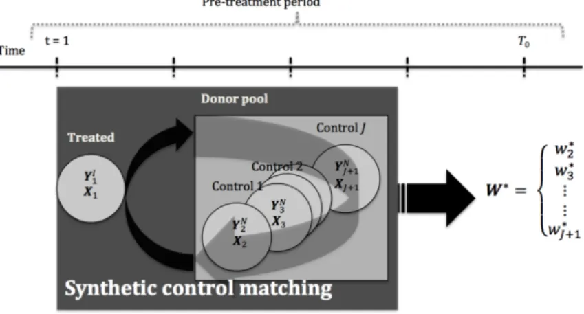
In order to run synthetic control method we suppose to collect the data on J + 1 units indexed by j = 1,...,J + 1. The data forms a balanced panel sample S, that is, no missing observations are present. Without loss of generality, we define that only the first unit j = 1is exposed to the treatment and is uninterruptedly exposed to the intervention of interest after some initial treatment period. This unit is described as treated (I)2_{. The rest of the units are the}_J _{potential controls (}_N₎3 that are not participating in the treatment and all of them constitute so-called “donor pool”4_{. Table}

2.1contains typical data set needed for theSCManalysis.

All the J + 1 units are observed over T periods, indexed by t = 1,...,T. The time period is divided in two subsequent periods. We suppose a positive number of pre-treatment periodsT0, for t = 1,...,T0, and a positive number of post-treatment periods T1, for t = T0+1,...,T, with

T = T0+T1and1  T0<T. This means that we do not have any interruption in observation and that there is at least one pre-treatment and one post-treatment period.

As already presented in section1.2.1, the variableYjt is the potential outcome and measures the impact of the treatment.YN

jt is the outcome that would be observed for the unit jat timetin the absence of the treatment.YI

jtis the outcome that would be observed for unit jat timetif the unit is exposed to the treatment in periodT0+1toT.

In addition to the outcome variable, we observe for each unit the confounding variables Cl_,

l = 1,...,m. The(m ⇥T)matrixCjcontainsmconfounding variablesCl. As we will see later in this section, we use the confounding variables to build the vector of observed covariatesZ.

2_{The index}_I_{as intervention.}

3_{The index}_N_{as non-intervention.}

(41)

2.2. Synthetic control methodology 23

Unit Identificator Time Outcome Confounders

j NAME t Y C1 _··· _Cm 1 Treated 1 .. . T0 T0+1 .. . T 9 > > = > > ; pre-treatment 9 > > = > > ; post-treatment Y11 .. . Y1T0 Y1T0+1 .. . Y1T 9 > > > > > > > > > > > > = > > > > > > > > > > > > ; Y1 C1 11 .. . C1 1T0 C1 1T0+1 .. . C1 1T ··· Cm 11 .. . Cm 1T0 Cm 1T0+1 .. . Cm 1T 2 Control 1 1 .. . T Y21 .. . Y2T 9 > > > = > > > ; Y2 C1 21 .. . C1 2T ··· Cm 21 .. . Cm 2T .. . ... ... ... ... ... ... J + 1 Control J 1 .. . T YJ+11 .. . YJ+1T 9 > > > = > > > ; YJ+1 C1 J+11 .. . C1 J+1T ··· Cm J+11 .. . Cm J+1T Source: Author’s elaboration.

Table 2.1: Data set Assumptions

As most of the program evaluation methods, theSCMis not an exception and is based on a couple of assumptions. The first assumption is defined as:

Assumption 4 (FirstSCMassumption).

We presume that the intervention does not have any effect on pre-treatment outcome and so we haveYN

jt =YjtI for allt 2 {1,...,T0}and j 2 {1,...,J + 1}. Note that in practice the treatment may have been anticipated and the impact on the outcome is visible before the selected treatment period. In this case, we can eventually redefine T0 as the first period in which the outcome may possible react to the treatment.

Furthermore, the second assumption on which is based the synthetic control method is defined as:

Assumption 5 (SecondSCMassumption).

We assume no interference between units (described in previous chapter by assumption1as

(42)

Treatment effect

We define byajt=YjtI YjtN the effect of the treatment for unit jat timet. The treatment effect for any unit and time period is represented by the figure2.1. Moreover, letDjtbe the causal exposure variable described in section1.2.1. We know that only the first unit is exposed to the treatment after periodT0, consequently, the causal exposure variable is redefined as:

Djt= 8 < : 1 if j = 1 and t > T0, 0 otherwise. (2.1)

Therefore the observed outcome for unit jat timetis:

Yjt=YjtN+ajt· Djt. (2.2)

As a result of equations (2.1) and (2.2), the treatment effect for unit j = 1at timet > T0is defined as:

a1t=Y1t Y1tN. (2.3)

Note that only theYN

1t is unobserved. The goal of the synthetic control method is to construct a synthetic control group providing an estimate for this missing potential outcome.

Source: Author’s elaboration.

(43)

2.2. Synthetic control methodology 25

Driving model

Synthetic control approach belongs to the class of difference-in-differences methods (for more details on the method see annexeA.1.1). It is a generalisedDID(fixed-effect) model that allows the effect of confounding unobserved characteristics to vary over time. In order to estimate the potential outcome of non-treated unit,YN

jt, based on a specific factor model5,Abadie et al. (2010) propose to use the weighted value of the outcome variable for each control from the donor pool that is:

J+1

Â

j=2

wjYjt,

wherewj is a value of the(J ⇥1)vector of weightsW = (w2, . . . ,wJ+1)0, s.twj 0andÂJ+1j=2wj=1. Each scalar wj represents the weight of unit jin the synthetic control. Each particular vector W generates one particular weighted average of control units, therefore one potential synthetic control. Ideally, we would like to choose among the set of all possibleWa vectorW⇤_{= (w}⇤

2, . . . ,w⇤J+1)0such that: J+1

Â

j=2 w⇤ jYjt=Y1t and J+1

Â

j=2 w⇤ jZj=Z1, 8t  T0. (2.4) Note that these conditions have to be true for all _{t  T}0, i.e. for all t in pre-treatment period. Moreover, if we ignore, for this moment, the mathematical optimisation procedure described in section 2.2.2, we can imagine the synthetic control matching procedure as a black box, and the results of it should be the set of weights W⇤_{. We represent the matching procedure graphically} by figure2.2. During the pre-treatment period, the treated unit j = 1is looking for the units in the donor pool that has similar characteristics. The results of the matching are the combination of the control units that the most resembles the treated unit before the treatment. For more details about the matching see annexeA.1.1.

If we suppose that there is suchW⇤ _{satisfying equations in (}_2.4_{), then under condition of no} extrapolation outside the convex hull of the data6_, _{Abadie et al.} ₍₂₀₁₀_{) suggest an estimator of} treatment effect (see equation (2.3)), defined as:

ˆ a1t=Y1t J+1

Â

j=2 w⇤ jYjt, 8t > T0. (2.5) Note that equations in (2.4) hold exactly if(Z0₁,Y11, . . . ,Y1T0)belongs to convex hull of{(Z02,Y21, . . . ,

Y2T0), . . . , (Z0J+1,YJ+11, . . . ,YJ+1T0)}. In practice, these equalities often do not hold, hence we have to make sure that the synthetic control is selected such that the equations in (2.4) hold approxima-tively7_.

5_{For more explanation see}_{Abadie et al.}₍₂₀₁₀_{, pp. 496).}

6_{For the proof see}_{Abadie et al.}₍₂₀₁₀_{, p. 504).}

7_{In addition, if our treated unit is an outlier (extreme value), the} _(Z0

1,Y11, . . . ,Y1T0) is to far of the convex hull of

(44)

Source: Author’s elaboration.

Figure 2.2: Synthetic control matching

Abadie et al. (2010) argue that synthetic control can provide useful estimates also in more

general context, for example, in the case of the autoregressive model with time-varying coefficients:

Yjt+1N = atYjtN+bt+1Zjt+1+ujt+1,

Zjt+1 = gtYjtN+PtZjt+njt+1,

whereujt+1andnjt+1have mean zero conditional onFt= Yjs,Zjs _{1 jJ+1,st}. If we suppose that we can choose{w⇤

j}2 jJ+1such thatÂJ+1j=2w⇤jYjT0=Y1T0 andÂJ+1j=2w⇤jZjT0=Z1T0, then we can prove that the synthetic control estimator is unbiased even if only one pre-treatment period is available8_.

Implementation of the driving model

Ideally, we would like to construct a synthetic control that most closely resembles the treated unit in all relevant pre-treatment characteristics. To do so,Abadie and Gardeazabal(2003) propose to make use of the observed characteristics of the units from the donor pool. They also propose to weight the pre-treatment outcomes and form linear combinations of these outcomes to control for unobserved common factors whose effects vary over time. Abadie and Gardeazabal(2003), and

Abadie et al.(2010) argue that if the pre-treatment period is large, then matching on pre-treatment

outcomes helps control for unobserved factor and the heterogeneity of the effect of the observed and unobserved factors on the outcome of interest. Moreover, they specify that only units that are alike in both observed and unobserved determinants of the outcome variables as well as in the