Influence of different digital terrain models (DTMs)on alpine permafrost modeling

Influence of different digital terrain models (DTMs)

on alpine permafrost modeling

Nadine Salzmann&Stephan Gruber& Marco Hugentobler&Martin Hoelzle

Received: 31 October 2004 / Revised: 1 February 2006 / Accepted: 1 May 2006 / Published online: 23 December 2006 # Springer Science + Business Media B.V. 2006

Abstract The thawing of alpine permafrost due to changes in atmospheric conditions can have a severe impact, e.g., on the stability of rock walls. The energy balance model, PERMEBAL, was developed in order to simulate the changes and distribution of ground surface temperature (GST) in complex high-mountain topography. In such environments, the occurrence of permafrost depends greatly on the topogra-phy, and thus, the digital terrain model (DTM) is an important input of PERMEBAL. This study investigates the influence of the DTM on the modeling of the GST. For this purpose, PERMEBAL was run with six different DTMs. Five of the six DTMs are based on the same base data, but were generated using different interpolators. To ensure that only the topo-graphic effect on the GST is calculated, the snow module was turned off and uniform conditions were assumed for the whole test area. The analyses showed that the majority of the deviations between the different model outputs related to a reference DTM had only small differences of up to 1 K, and only a few pixels deviated more than 1 K. However, we also observed that the use of different interpolators for the generation of a DTM can result in large deviations of the model output. These deviations were mainly found at topographically complex locations such as ridges and foot of slopes.

Keywords complex topography . digital terrain model (DTM) . high mountain permafrost . modeling . sensitivity

1 Introduction

Permafrost is a widespread phenomenon in high-mountain environments such as the European Alps [18]. It is defined as lithospheric material that remains at or below a temperature of 0°C for at least 1 year [29]. In complex mountain to-pography, permafrost can stabilize infrastructure, rock walls and debris-covered slopes [5,7,9]. The close link between permafrost and the atmosphere, together with permafrost temperatures that in the European Alps are often close to melting conditions, makes permafrost especially sensitive to climatic changes. As a result, some permafrost is thawing [1, 6,10], resulting in severe slope stability problems and other adverse ecological consequences [1, 3, 7, 9]. In high-mountain regions with intense human activities such as in the Alps, permafrost degradation has increased the risk of permafrost-related hazards [14, 16, 24, 32]. Therefore, knowledge of the distribution and dynamics of permafrost is important in order to develop mitigation strategies.

To simulate the distribution and changes of alpine permafrost the process-based energy balance model PER-MEBAL was developed [4,23,28]. PERMEBAL is able to calculate the average ground surface temperature (GST), which is an indicator of the presence or absence of permafrost. In complex high-mountain topography, the microclimate, and thus the permafrost distribution, is strongly dependent on topoclimatic factors [19]. Therefore, the digital terrain model (DTM) is a key input variable of PERMEBAL [28]. The study of Hoelzle [11], for example, showed that the horizontal resolution of the DTM has a significant influence on the calculation of the solar radiation

N. Salzmann (*)

:

:

Glaciology and Geomorphodynamics Group, University of Zurich, Winterthurerstrasse 190, CH-8057 Zurich, Switzerland

e-mail: nsalzman@geo.unizh.ch M. Hugentobler

Geographic Information Systems Division, University of Zurich, Winterthurerstrasse 190, CH-8057 Zurich, Switzerland

in mountain environments, and thus, on the modeled permafrost distribution. Hence, we assume that the DTM significantly affects the calculation of the average GST. Latest research in the field of digital terrain modeling offers a range of sophisticated triangle-based terrain models [13], which can be used as input for PERMEBAL.

This study evaluates the sensitivity of simulated GSTs on the use of various DTM inputs. To date, only the DTM ‘DHM25’ (see below) has been used for alpine permafrost modeling on the decameter scale. Therefore, in this study, the uncertainties of the modeled GST outputs caused by the application of six different high-resolution DTMs are analyzed and discussed.

2 Data and models

2.1 Study site

The sensitivity study was carried out within the Corvatsch area (Upper Engadine) of Switzerland, one of the most frequently investigated mountain permafrost sites in the Alps [12]. The climate in this part of the Alps is slightly continental and mainly influenced by SW air masses. The mean annual precipitation in the periglacial area is about 1,000–2,000 mm [27] and the mean annual 0° isotherm lies at around 2,200 m asl. The test area (782400/142400 and 783900/145000) covers the station Corvatsch, Piz Murtèl and the rock glacier Murtèl (figure1).

2.2 The digital terrain models

The DTMs applied in this study have a horizontal resolution of 10 m. To allow an accurate comparison, the same spatial

resolution was used for each DTM. Furthermore, except for the ph (for details, see below), base data are provide by the DHM25 for all the other DTMs; these data are owned and supplied by the swisstopo (Swiss Federal Office of Topography, Berne). Therefore, these five DTMs differ only through their interpolators. In the following, a short introduction is given about the basis for and interpolation methods used for the raster calculation of the DTMs.

d10 is the resampled DHM25. The original DHM25 has a horizontal resolution of 25 m. The base data for the DHM25 are digitized contours, peaks, breaklines and lake borders. The calculation of a 25-m raster from these data has been performed by using a search-ray-based approach. From every raster point, a number of search rays pointing in different directions are used to locate intersections with contours. Spline curves were then fitted to the rays and their elevations averaged at the raster point [26]. These data were resampled to a 10-m resolution by applying bilinear interpolation in order to produce d10.

ph is a photogrammetrically derived DTM. It is based on two scanned infrared aerial photographs and was automat-ically derived by using the digital photogrammetrical software SOCET SET from the Leica–Helava system [17]. This technique is based on studying the differences in the optical contrasts of the aerial photographs. The two aerial photographs delivered by swisstopo were taken at the end of the hydrological year (7 September 1988) in order to ensure a maximum snow-free state. However, the glaciers in the area are still snow-covered. The DTM was computed by A. Kääb, University of Oslo.

For the following triangle-based interpolators (li, co, ct, sc), the DHM25 base data have been tessellated with a constrained Delaunay triangulation. This ensures that no triangle edge crosses a contour or a breakline.

li – the triangles have been interpolated linearly, and thus gradient and aspect are constant within one facet. co – a cubic Coons interpolator was applied over triangular patches. The resulting surface is one time continuously differentiable. To better represent sharp features in high-mountain areas, a breakline extension was used [13]. As a result, the surface is continuous across breaklines, but not continuously differentiable. ct – a cubic interpolator based upon Clough–Tocher triangles [2]. The surface is also one time continuously differentiable and a breakline extension similar to the Coons patch was used. The derivatives orthogonal to the triangle boundary curves are linearly interpolated. sc – a smoothed version of the Clough–Tocher interpolant. The derivatives orthogonal to the triangle boundary curves were interpolated in a way that the curvature change at the border of the triangles is slower than with linearly interpolated cross-derivatives [13]. The DTMs d10 and ph only provided the surface parameter elevation. The calculations of‘slope’ and ‘aspect’ were performed using the commands slope and aspect within the software package ArcINFO (ESRI). The surface parameters slope and aspect of the triangulated irregular network (TIN)-based DTMs were calculated directly from the surface.

2.3 The energy balance model PERMEBAL

The energy balance model PERMEBAL simulates the main energy exchange processes between the atmosphere and the surface, and includes calculations for shortwave net radiation, longwave incoming and emitted radiation, turbu-lent fluxes and snow distribution [4,23,28]. In addition to the data from the DTM, the model is driven with meteorological time series and ground surface character-istics (figure2). After providing this set of input data, the 2D version of PERMEBAL, which we use in this study, is able to simulate the distribution and changes of daily GST in complex high-mountain topography at a local to regional scale.

2.4 The PERMEBAL runs

The six model runs were all performed with the same settings. For this study, a 5-year simulation (according to the hydrological year) was conducted and initiated in 1998. The meteorological input data were provided by MeteoSwiss (Swiss Federal Office of Meteorology and Climatology, Zurich) from their meteorological station at Piz Corvatsch (3,315 m asl, 783160/143525).

Snow has a strong impact on the seasonal thermal regime [19] due to its low thermal conductivity, which

makes it a good insulator [15,20,30,31]. Hence, seasonal snow cover modifies the topographic feedback signal. This study assesses the influence of the topographic input only. Therefore, the snow module was turned off to ensure that only the topographic effect on surface temperature is calculated, and thus PERMEBAL does not take snow cover into account.

Similar to the snow cover, local surface conditions, such as vegetation and subsurface layers like organic matter, coarse blocks or glaciers, act as a buffer between the atmosphere and the ground [8,21]. Therefore, the potential effects of these factors were also eliminated and a rock surface was assumed for the entire test region.

By ignoring the snow cover and by using uniform surface characteristics, comparable conditions for all parameters over the entire test region are given. Hence, no other signals are included than those of the various DTMs, thereby allowing us to assess the sensitivity of PERMEBAL to these inputs.

3 Results

Results are divided into three sections and presented as follows: First, elevation (Section3.1.1), slope (Section3.1.2) and aspect (Section 3.1.3) of the different DTMs are com-pared, as well as the modeled average GST (Section3.1.4). Second, the locations of the differences in the model outputs using image subtractions are reported. Finally,

Figure 2 Schematic of PERMEBAL as applied in this study (after Stocker-Mittaz et al. [28]). The input that was varied for this study is bold-bordered, and those, which were kept equal during all inves-tigations, are normal-bordered. The calculation steps that were omitted, are dash-bordered or are in italic letters

transect analyses are performed on two areas selected on the basis of the findings reported in the first two sections.

3.1 Comparison of the DTM surface parameters and the resulting modeling outputs (value ranges and frequency values)

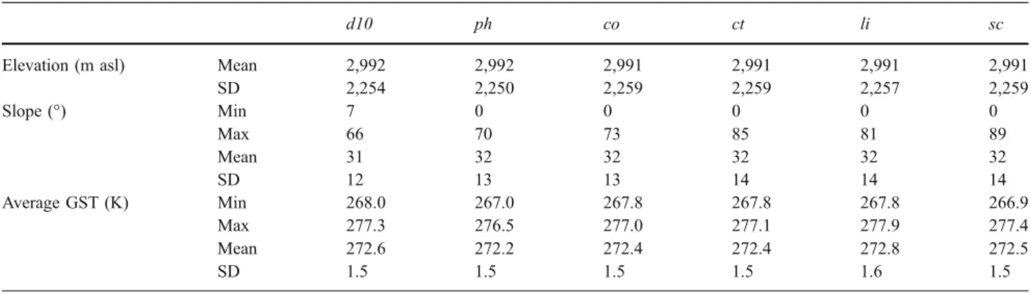
A first, general impression as well as a comparison of the applied DTMs and the model output (average GST) is given by the analyses of their value ranges (see table 1) and frequency values (see figure3) over the entire test area.

3.1.1 Elevation

The range of mean elevation values and standard deviations for the entire test area are summarized in table 1. Differ-ences between the ranges are small. The mean elevations and standard deviations vary within only 1 and 9 m, respectively. The frequency curves for the elevation (figure 3a) also show only small variations between the six DTMs. Therefore, as these marginal differences in elevation do not significantly influence the resulting GST, they will not be a major focus in this paper.

3.1.2 Slope

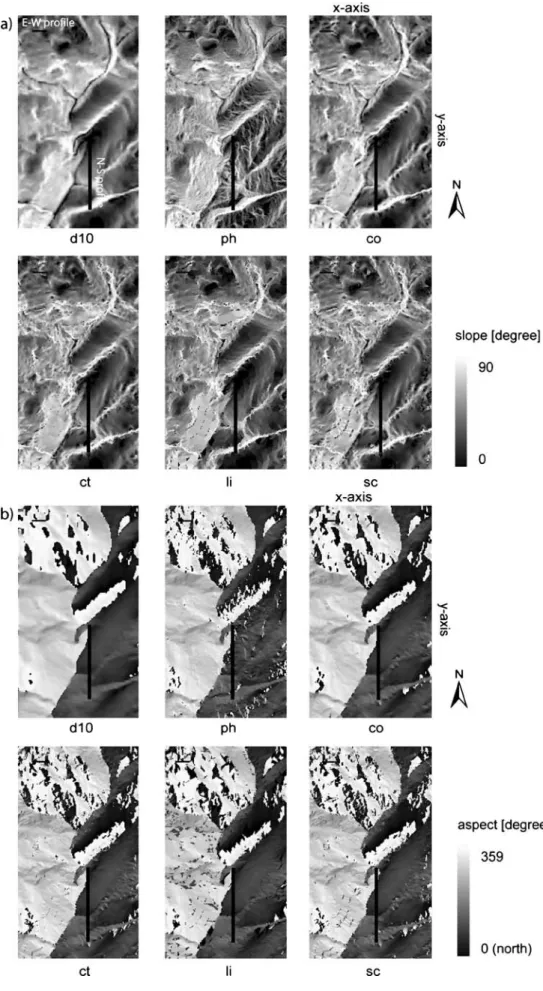
Differences between the slope samples are far greater than those for the elevations. The differences in slope maxima vary by up to 23° (table 1) and the frequency curves also show considerable variations (figure 3b). The majority and also the highest differences occur between about 20° and 45° (figure 3b). The image plots of slope (figure 4a) also reveal significant differences and notable slope patterns appear in d10, ph and li. The pattern of d10 is very smoothed and is caused by the spatial resampling applied. In contrast, the pattern of ph displays large differences between neighboring pixels in the snow-covered areas. This is probably caused by the snow cover

(see above and the discussion). Finally, li has quite a patchy pattern.

3.1.3 Aspect

The distributions of the aspect frequency (figure 3c) are quite similar apart from co and especially the li, where some single data values are either very frequent or rare in comparison to the others. These very high frequency values are all N-exposed. Most similarities between the frequency curves are found between about 150° and 250° (south sector). At the same time, the south exposition is least represented in our test area. The image plots of aspect (figure 4b) show similar distinctive feature as the slope images (figure 4a). d10 is very smooth, ph shows an unsettled image in the glacier area and li has large aspect variations in the westerly part.

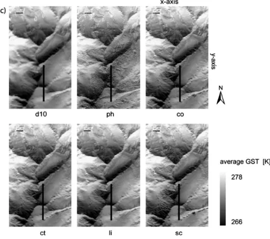
3.1.4 Average ground surface temperature

The modeled GSTs show differences for the minima of 1.1 K and for the maxima of 1.4 K. These values are related to single pixel values, and thus are not so important. The mean values differ within 0.6 K (table 1). The frequency curves all have quite similar progression; however, note how the curves shift vertically between about 271 and 273 K (figure3d).

On the output images (figure 4c), the patterns of the surface parameters elevation, slope and aspect are well reflected in the pattern of the modeled average GST and therefore, their relationship to elevation is clear. Moreover, the pattern of slope is reflected in the model output, particularly in the image of ph, where the noisy pattern of slope is well recognizable in the pattern of the average GST. Furthermore, the patchy slope pattern of li is also reflected in the corresponding image of the average GST. Finally, the pattern of the aspect over the entire test area is also apparent in the modeled results.

Table 1 Value ranges of surface parameters for each DTM over the entire test area.

d10 ph co ct li sc

Elevation (m asl) Mean 2,992 2,992 2,991 2,991 2,991 2,991 SD 2,254 2,250 2,259 2,259 2,257 2,259 Slope (°) Min 7 0 0 0 0 0 Max 66 70 73 85 81 89 Mean 31 32 32 32 32 32 SD 12 13 13 14 14 14 Average GST (K) Min 268.0 267.0 267.8 267.8 267.8 266.9 Max 277.3 276.5 277.0 277.1 277.9 277.4 Mean 272.6 272.2 272.4 272.4 272.8 272.5 SD 1.5 1.5 1.5 1.5 1.6 1.5

3.2 Deviation detection using difference images

For the following analyses, a reference DTM was selected. In respect to choice of the reference DTM, we have taken into account practical aspects, because an objective criteri-on, such as accuracy or quality is lacking. The DHM25 is the only commercial DTM within our sample, and thus probably the most frequently used in Switzerland. Hence, we have chosen d10 as the reference DTM since it is the closest derivative of the DHM25. We have assumed that it would be most interesting to know, where and how large the deviations are, if alternative DTMs from d10 are used as model input. The locations and absolute values of the deviations that result, when PERMEBAL is run with the different DTM inputs, were detected by subtracting the output images from each other.

The basic statistics (min, max, mean, SD) are summa-rized in table 2. The pixel-by-pixel-based minimum and maximum deviations are within−3.9 and 5.4 K, and have a mean value between −0.2 and 0.4 K. The standard deviation is very similar for all subtraction images (about 0.5 K), with only ph showing a higher value of 0.8 K.

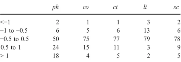
The detected areas of deviation are shown in figure5, and the absolute values of the percentage deviations are

listed in table 3. The ranges of deviation were classified into three groups: (1) ‘high deviation pixels’ with a deviation of the calculated average GST of more than ±1 K compared to the output modeled with d10; (2) ‘moderate deviation pixels’ with a deviation between −1 to −0.5 K and 1 to 0.5 K, respectively; and (3) ‘low deviation pixels’ with a deviation of less than ±0.5 K.

Comparing the number of ‘high deviation pixels’ of the different model outputs, we found that the output based on ph counts most pixels (20%) in this class (figure 5). Only 50% of the pixels are classified as ‘low deviation pixels’, and 30% are in the class of ‘moderate deviation pixels’. The positive deviation pixels are mainly located at the S-exposed sections and the highest deviations tend to be near the ridges. The spatial distribution of the negative deviation pixels is more dispersed. However, there is also a tendency for them to be located near or at the ridges.

The subtraction images of co, ct and sc show similar, but much less distinct tendencies, in particular for sc and ct, where the highest negative deviation pixels are not primarily found at the ridges. In these model outputs, the negative-deviation pixels are mainly located at the NE–N slopes and in the lower elevated NW corner of the test area.

Figure 4 2D image plots of slope (a), aspect (b) and the modeled average GST (c). The black bars show the location of the horizontal and vertical pro-files that are investigated in section3.3

Most of the positive-deviated pixels are found in the SE– S–SW exposition and at the ridges.

When comparing the simulation run of li with that of d10, we find that most of the pixels (79%) were classified as ‘low-deviation pixels’. In contrast to the other subtrac-tion images, more pixels (13%) were classified as ‘moder-ate- (negative-) deviation pixels’. The negative deviation part of this class is dispersed over the whole test site with the highest negative deviations to be mainly found, similar with the other subtraction maps, at the ridges and in the NW corner. The positive deviation pixels are found almost only at the ridges.

In general, most of the deviation pixels and, in particular, those with the highest absolute values, are found at topographically complex sites like ridges or foot of slopes.

3.3 Profiles

One profile was extracted in each of the two areas where the main deviations have been located. An E–W one (figures 4 and 6a) through the lower elevated NW corner where some large deviations have been found between the model outputs, and a N–S one (figures 4 and 6b) through the high elevated regions where many ridges exist and the deviations were mainly relatively high.

The two profiles show the causes of deviations in the modeled average GST. In general, it is recognizable that when the curves of slopes from the different DTMs and also those of aspect are similar, then the differences between the curves of average GST are also low (figure6a,b). The analyses in more details are given below. In the E–W profile (figure6a) between 25 and 32 on the x-axis, the average GST varies by up to 2 K between the DTMs. This is mainly caused by li and ph, with other profile curves of slope and aspect not having strong deviations. From about 33 to 40 along the x-axis, the slope curves vary quite strongly and the aspects change frequent-ly between NE and NW. However, as in the section before, in the average GST, only li and ph deviate significantly. Within about 42 to 50 on the x-axis, the average GST is quite similar for all DTMs, and the profiles of slope and

Figure 4 (Continued)

Table 2 The deviations of the image subtraction related to d10. ph co ct li sc Average GST (K) Min −3.7 −3.5 −3.5 −3.9 −3.7

Max 4.9 4.9 4.6 4.6 5.4 Mean 0.4 0.2 0.2 −0.2 0.1 SD 0.8 0.5 0.5 0.5 0.5

aspect also show very low deviations. From 55 to about 59 on the x-axis, the average GST is again quite similar for all DTMs apart from d10 and ph, which have substantially less steep slope in this section and NE aspect. The co in this section is also NE-exposed, but the slope is only moder-ately steep. Nevertheless, the average GST of co is very close to those of ct, li and sc. After about 60 along the x-axis until 68, the curve progressions are quite similar apart from those of ph and ct at around 60 on the x-axis. In the very last section, the aspect of d10, li and ph are NW, while the others change to NE. The slope values are quite similar for all DTMs. With the change form NW to NE, the related curves of the average GST rise about 1 K.

In the N–S profile, which is located in the glacierized area, the most noticeable point is the high variability of all of the ph profile curves. Between about 150 and 170 on the y-axis, the slope curves are quite similar apart from d10 and ph. The aspect curves of li and ph change in this section between NW and NE. The resulting average GSTs are quite similar apart from d10. In the sections, where the curves of

slope and aspect have quite a similar form (about 170 to 220 along the y-axis), the curves of the average GST are also quite equal or at least parallel. Between about 230 and 240 on the y-axis, the slopes and aspects are also quite similar. The curves of the resulting average GST in this section, however, have a similar progression but are parallel-shifted. The motion of the slope and the aspect curves are reflected in the average GST between 210 and 240 on the y-axis. However, in this section and in general, it seems that aspect has a slightly stronger impact on the average GST than slope.

4 Discussion and conclusions

The purpose of this study was to assess the sensitivity of the energy balance model PERMEBAL to various DTM inputs. The mean average GST over the entire test area varies only within 0.6 K. The pixel values of the average GST modeled with d10 as compared with those modeled using the other DTMs, showed in general low deviations. About 75–79% of the calculated average GST (except for ph with only 50%) were in the class of ± 0.5 K (low-deviation pixels). At the locations of this class, the differences in elevation, slope and aspect between the different DTMs were also low. Only 1–5% of the total number of pixels in the test area (except for ph where this increased to 18%) deviated more than ±1 K (class of high-deviation pixels). These pixels were located mainly at the ridges, and thus at locations of most complex topography. These sites were expected to be most critical, since here significant topographical changes occur within very short spatial distance. Furthermore, such areas represent extreme locations also from the geological and (micro-) climatolog-ical point of view. Therefore, the uncertainties at such locations will always be the greatest, due to uncertainties in the topographical input as well as difficulties in modeling the physical processes. Here, deviations of up to 5.4 K for single pixel values resulted between calculations made with d10 compared to calculations made with the other DTMs.

The differences in aspect, in particular when a change from N to S or from W to E and vice versa is included, have led to high deviations. Furthermore, S-exposed areas

Figure 5 3D plots of the subtraction maps

Table 3 Deviation (%) of average GST (K) from d10.

ph co ct li sc <−1 2 1 1 3 2 −1 to −0.5 6 5 6 13 6 −0.5 to 0.5 50 75 77 79 78 0.5 to 1 24 15 11 3 9 > 1 18 4 5 2 5

seem to be slightly more sensitive to topographical variations; this phenomenon can be explained by the higher amount and importance of incoming radiation in the energy balance of south aspect slopes. The influence of slope seems to play a less dominant role than aspect.

The high-deviation single-pixel values are mainly found at topographically complex sites like ridges or foot of slopes. Such areas represent extreme locations also from a geomorphological and (micro-) climatological point of view. Hence, not only the topographical input data have the most uncertainties in these areas, but also the modeling of the energy balance will be most critical at such locations.

Therefore, the results of PERMEBAL should be treated with particular care in such areas.

We have seen that the average GSTs modeled with the photogrammetrically derived DTM (ph) differ significantly from those modeled with other DTMs. This result is to be expected since each DTM, except ph, is based on the same base data. Because of the equal base date, the deviations in the PERMEBAL output are only caused by the different interpolation techniques that were used to generate the DTMs. Furthermore, the majority of the deviation pixels of ph are located in the glacierized, snow-covered areas. This can be explained by the compilation technique of the ph DTM and

the specific natural circumstances at the time of taking the aerial photograph. The technique of photogrammetrically deriving DTM is based on optical contrasts. However, the optical contrasts are generally reduced in infrared photo-graphs and even more reduced or almost non-existent over snow-covered areas or glaciated areas [22]. Without strong optical contrast, the calculation of the elevation is difficult and this can lead to miscalculations. Therefore, the major part of the deviation pixels in this area can be explained with the weakness of photogrammetrically derived DTMs from infrared photographs, especially over snow-covered areas.

5 Perspectives

In this study, six different DTMs were used to assess the influence of topographic input on each of these specific DTMs. Further analysis of the sensitivity of PERMEBAL should be carried out. As an example, artificial DTMs should be used with a topography that represents ‘moun-tains’ in an idealized geometrical form, e.g., a cone or a cylinder. In this way, the influence of the topography can be analyzed using a more systematic approach.

In a similar manner, sensitivity studies should be conducted that include snow cover and different surface characteristics. Therewith, the effect of these buffer layers on the influence of the topographic input can be assessed.

In the context of climate change and its impact on alpine permafrost, further studies are needed that link PERME-BAL with scenario output from Regional Climate Models (RCMs) [25]. Such model combinations offer promising perspectives; however, they should also include knowledge about the uncertainties caused by the DTM applied.

Acknowledgments This study was made possible thanks to the European Cooperation in the field of Scientific and Technical Research (COST-Action 719). We gratefully acknowledge the review of the manuscript by I. Woodhatch, the critical comments of W. Haeberli (both at University of Zurich), the support of A. Kääb (University of Oslo) concerning questions in photogrammetry, and the very valuable comments of one of the anonymous reviewers.

References

1. Davies, M. C. R., Hamza, O., & Harris, C. (2001). The effect of rise in mean annual temperature on the stability of rock slopes containing ice-filled discontinuities. Permafrost and Periglacial Processes, 12(1), 137–144.

2. Farin, G. (1997). Curves and Surfaces for CAGD: A Practical Guide. San Francisco, CA: Morgan Kaufmann.

3. Gruber, S., Hoelzle, M., & Haeberli, W. (2004). Permafrost thaw and destabilization of alpine rock walls in the hot summer of 2003. Geophysical Research Letters, 31(13), L13504.

4. Gruber, S., Hoelzle, M., & Haeberli, W. (2004). Rock-wall temperatures in the Alps: Modelling their topographic distribution and regional differences. Permafrost and Periglacial Processes, 15(3), 299–307.

5. Haeberli, W. (1992). Construction, environmental problems and natural hazards in periglacial mountain belts. Permafrost and Periglacial Processes, 3(2), 111–124.

6. Haeberli, W., & Beniston, M. (1990). Climate change and its impact on glaciers and permafrost in the Alps. Ambio, 27(4), 258–265. 7. Haeberli, W., Wegmann, M., & Vonder Muehll, D. (1997). Slope

stability problems related to glaciers shrinkage and permafrost degradation in the Alps. Eclogae Geologicae Helvetiae, 90, 407–414. 8. Harris, C., & Pedersen, D. (1998). Thermal regimes beneath coarse blocky materials. Permafrost and Periglacial Processes, 9(2), 107–120. 9. Harris, C., Rea, B., & Davies, M. (2001). Scaled physical modelling of mass movement processes on thawing slopes. Permafrost and Periglacial Processes, 12(1), 125–135.

10. Harris, C., Vonder Muehll, D., Isaksen, K., Haeberli, W., Sollid, J. L., & King, L. (2003). Warming permafrost in European mountains. Global and Planetary Change, 39, 215–225. 11. Hoelzle, M. (1994). Permafrost und Gletscher im Oberengadin,

Vol. 132. Switzerland: Mitteilungen VAW/ETH Zurich.

12. Hoelzle, M., Vonder Muehll, D., & Haeberli, W. (2002). Thirty years of permafrost research in the Corvatsch–Furtschellas area, Eastern Swiss Alps: A review. Norwegian Journal of Geography, 56, 137–145.

13. Hugentobler, M. (2004). Terrain modelling with triangle based free-form surfaces, PhD thesis, Department of Geography. Switzerland: University of Zurich.

14. Huggel, C., Haeberli, W., Kääb, A., Bieri, D., & Richardson, S. (2004). Assessment procedures for glacial hazards in the Swiss Alps. Canadian Geotechnical Journal, 41(6), 1068–1083. 15. Ishikawa, M. (2003). Thermal regimes at the snow–ground

interface and their implications for permafrost investigation. Geomorphology, 52(1–2), 105–120.

16. Kääb, A., Reynolds, J. M., & Haeberli, W. (2005). Glacier and permafrost hazards in high mountains. In U. M. Huber, M. A. Reasoner, & B. Gugmann (Eds.), Global change and mountain regions: A state of knowledge overview. Advances in global change research (pp. 225–234). Dordrecht: Kluwer Academic Publishers.

17. Kääb, A., & Vollmer, M. (2000). Surface geometry, thickness changes and flow fields on creeping mountain permafrost: Automatic extraction by digital image analysis. Permafrost and Periglacial Processes, 11, 315–326.

18. Keller, F., Frauenfelder, R., Gardaz, J. M., Hoelzle, M., Kneissel, C., Lugon, R. (1998). Permafrost map of Switzerland, In Proceedings of 7th International Conference on Permafrost, Vol. 57(pp. 557–562). Canada: Yellowknife.

19. Keller, F., & Gubler, H. (1993). Interaction between snow cover and high mountain permafrost, Murtèl–Corvatsch, Swiss Alps, In Proceedings of 6th International Conference on Permafrost, Vol. 1 (pp. 332–337) July 5–9, Beijing, PR China.

20. Ling, L., & Zhang, T. (2004). A numerical model for surface energy balance and thermal regime of the active layer and permafrost containing unfrozen water. Cold Region Science and Technology, 38(1), 1–15.

21. Luthin, J., & Guymon, G. (1974). Soil moisture–vegetation– temperature relationships in central Alaska. Journal of Hydrology, 23, 233–246.

22. Lutz, E., Geist, T., & Stoetter, J. (2003). Investigations of airborne laser scanning signal intensity on glacial surfaces – Utilising comprehensive laser geometry modeling and orthophoto surface modeling (A case study: Svartisheibreen, Norway), In Proceed-ings, ISPRS Workshop on 3-D reconstruction from airborne laserscanner and INSAR data. Germany: Dresden.

23. Mittaz, C., Imhof, M., Hoelzle, M., & Haeberli, W. (2002). Snowmelt evolution mapping using an energy balance approach over an alpine terrain. Arctic, Antarctic and Alpine Research, 34 (3), 274–281.

24. Noetzli, J., Hoelzle, M., & Haeberli, W. (2003). Mountain permafrost and recent alpine rock fall events: A GIS-based approach to determine critical factors. In Proceedings of 8th International Conference on Permafrost, Vol. 1, (pp. 827–832) July 20–25, Zurich, Switzerland.

25. Salzmann, N., Frei, C., Vidale, P. L., Hoelzle, M. The application of Regional Climate Model output for the simulation of high-mountain permafrost scenarios. Global and Planetary Change (in press).

26. Schneider, B. (1998). Geomorphologisch plausible Rekonstruk-tion der digitalen RepraesentaRekonstruk-tion von Gelaendeoberflaechen aus Hoehenliniendaten, PhD thesis, Department of Geography. Swit-zerland: University of Zurich.

27. Schwarb, M., Frei, C., Schaer, C., & Daly, C. (2000). Mean annual precipitation throughout the European Alps 1971–1990, In:

Hydrological Atlas of Switzerland. Bern: Landeshydrologie und Geologie.

28. Stocker-Mittaz, C., Hoelzle, M., & Haeberli, W. (2002). Model-ling alpine permafrost distribution based on energy-balance data: A first step. Permafrost and Periglacial Processes, 13, 271–282. 29. Washburn, A. L. (1997). Geocryology: A Survey of Periglacial

Processes and Environments. London: Arnold Ltd.

30. Zhang, T., Barry, R. G., & Haeberli, W. (2001). Numerical simulation of the influence of the seasonal snow cover on the occurrence of permafrost at high altitudes. Norwegian Journal Geography, 55, 261–266.

31. Zhang, T., Osterkamp, T. E., & Stamnes, K. (1996). Influence of the depth hoar layer of the seasonal snow cover on the ground thermal regime. Water Resources Research, 32, 2075–2086. 32. Zimmermann, M., & Haeberli, W. (1992). Climatic change and

debris flow activity in high mountain areas: A case study in the Swiss Alps. In M. Boer & E. Koster (Eds.), Greenhouse-Impact on Cold-Climate Ecosystems and Landscapes. Catena Supple-ment, 22, 59–72.