Active Learning Using Meta-Learned Priors
by
Paolo Gentili
Submitted to the Department of Electrical Engineering and Computer
Science
in partial fulfillment of the requirements for the degree of
Master of Engineering in Electrical Engineering and Computer Science
at the
MASSACHUSETTS INSTITUTE OF TECHNOLOGY
September 2019
c
○ Massachusetts Institute of Technology 2019. All rights reserved.
Author . . . .
Department of Electrical Engineering and Computer Science
August 23, 2019
Certified by . . . .
Leslie P. Kaelbling
Panasonic Professor of Computer Science and Engineering
Thesis Supervisor
Certified by . . . .
Tomás Lozano-Pérez
School of Engineering Professor in Teaching Excellence
Thesis Supervisor
Accepted by . . . .
Katrina LaCurts
Chair, Master of Engineering Thesis Committee
Active Learning Using Meta-Learned Priors
by
Paolo Gentili
Submitted to the Department of Electrical Engineering and Computer Science on August 23, 2019, in partial fulfillment of the
requirements for the degree of
Master of Engineering in Electrical Engineering and Computer Science
Abstract
Deep learning models have found enormous success across a variety of displines, but training the parameters within these models generally requires huge amounts of la-belled data. One technique to reduce the burden of this data requirement is meta-learning, which involves extracting knowledge from previously experienced tasks so we can train new tasks with less data. Another such technique is active learning, where we selectively query labels for examples to train on, which potentially allows us to train a new task with fewer labelled data points. We investigate the potential to use active learning in the meta-learning setting, combining the advantages of the two techniques and further reducing the requirements for labelled data. In particular, we consider several techniques for actively querying labels within the modular meta-learning framework. We apply these techniques to several empirical settings, finding significant advantages over a baseline of random queries.
Thesis Supervisor: Leslie P. Kaelbling
Title: Panasonic Professor of Computer Science and Engineering Thesis Supervisor: Tomás Lozano-Pérez
Acknowledgments
First and foremost, I would like to thank my mentor Ferran Alet for his never-ending guidance and patience throughout this entire process. For always making time to meet and explain things, checking up on me and providing gentle nudges in the right direction, and providing the vision needed to make this project possible, thank you.
A big thank you to my thesis advisors, Professors Leslie Kaelbling and Tomás Lozano-Pérez, for welcoming me into their lab and for fostering such a friendly and collaborative lab culture. Thank you Professor Kaelbling for also being an amazing role model to me as a teacher during my time as a TA.
Thank you to my fellow UROP and MEng students who have helped pass the time on many a day in lab this past summer.
Thank you to all of my friends at MIT, who have made the past five years here all worth it.
Thank you to my parents and my brother, for always supporting me and providing me with much-needed advice, both in my academic career and in life. Your steadfast presence gives me comfort wherever my choices in life may take me.
A final thanks goes to the MIT Supercloud, whose computational resources made this research possible [25].
Contents
1 Introduction 13
1.1 Motivation . . . 13
1.2 Problem Description and Our Approach . . . 14
2 Meta-Learning 15 2.1 Description . . . 15
2.2 General Formulation . . . 16
2.3 Meta-Learning Example: Few-Shot Learning . . . 18
2.4 Prior Work . . . 19 2.4.1 Model-Agnostic Meta-Learning . . . 19 2.4.2 Modular Meta-Learning . . . 20 3 Active Learning 23 3.1 Description . . . 23 3.2 General Formulation . . . 24 3.3 Prior Work . . . 24 3.3.1 Uncertainty Sampling . . . 25
3.3.2 Query-by-Committee and Disagreement-Based Methods . . . . 26
3.3.3 Variance Reduction and the Cohn Criterion . . . 28
4 Joining Meta-Learning and Active Learning 31 4.1 Prior Work . . . 31
4.1.2 Probabilistic Model-Agnostic Meta-Learning . . . 35
4.2 Our Method: Modular Meta-Learning . . . 36
4.2.1 Variance . . . 37
5 Experiments and Results 39 5.1 Alet Function Regression . . . 39
5.1.1 Summed Function Regression Problem . . . 39
5.2 Omnipush Dataset . . . 42
5.2.1 Dataset Description . . . 42
5.2.2 Meta-Learning Problem . . . 42
List of Figures
2-1 Meta-training and meta-testing both contain sets of tasks to be com-pleted, each task comprising a traditional learning problem with train-ing and test sets. Figure from Finn’s “Learntrain-ing to Learn” (2017) [7], adapted from Ravi & Larochelle (2017) [24] . . . 19 5-1 Sample modules after the meta-training phase. . . 40 5-2 A visualization of the initial prior (uniform) distribution over
struc-tures, and the posterior distributions, as an active learner queries new points (in red) using variance (left) and the Cohn criterion (right). Darker lines correspond to structures assigned higher probabilities. . . 41 5-3 A plot of mean squared error by number of queries for the Alet function
dataset, with error bars of 1 standard deviation. . . 42 5-4 An example Omnipush object displaying the four different attachments
and an extra weight. Figure from Bauza et al. (2018) [3] . . . 43 5-5 A plot of mean squared error by number of queries for the Omnipush
dataset, with error bars of 1 standard deviation. . . 44 5-6 A display of the first 8 pushes (in black) queried by the variance (top
left), entropy (top right), and Cohn (bottom) active learning criteria for an Omnipush example. . . 45
List of Tables
5.1 Mean squared error (×10−2) for random queries and different active learning criteria in the Alet function dataset. Numbers in bold are not significantly different from the best technique for that number of queries. 41 5.2 Mean squared error for random queries and different active learning
cri-teria for the Omnipush dataset. Numbers in bold are not significantly different from the best technique for that number of queries. . . 43
Chapter 1
Introduction
1.1
Motivation
In many modern machine learning applications involving large parametric models, training requires large amounts of both computational power and labelled training data [15, 29]. While the rise of GPUs (graphics processing units) and TPUs (tensor processing units) [13] has given us the ability to train larger and more complex models, obtaining labelled data remains a constant challenge.
Labeling training data is generally costly and time consuming; it can require humans to manually provide target labels, as is the case for image classification or segmentation tasks, or involve physical experiments to gather target labels. This latter case is particularly relevant for certain areas of robotics, where a robot must interact with physical objects. Here, researchers must manually reset the environment before allowing the robot to run, and each of these runs can be lengthy, especially when compared to simulation. Combined with the propensity of robots to break down, this leads to a significant barrier to data collection.
Thus, there is clear motivation to formulate learning algorithms that can perform well with small amounts of data, or otherwise intelligently query labels of data that it will use to train the model.
1.2
Problem Description and Our Approach
In this thesis, we consider the data burden of building an intelligent robot that can function in a variety of household scenarios. Given the diversity of situations that a human encounters day to day, such a robot would need to successfully perform a multitude of tasks and additionally be adaptable to the spontaneity of events that occur during daily life. In such a setting, it is infeasible to use pure supervised learning to train this robot, since the robot must be able to learn new tasks quickly and from small amounts of data.
We combine two techniques that are well-suited to this issue: meta-learning and active learning, both of which help reduce the data requirements associated with learning a new task. Specifically, meta-learning allows us to take advantage of the experience and knowledge we have acquired from learning previous tasks in order to more quickly learn the new task. Active learning allows us to be more discerning in the data points we choose to query; by intelligently and adaptively querying labels to the data points we would like to train on, we can significantly reduce the amount of supervision needed to achieve high performance on a new task.
Traditionally, meta-learning and active learning are considered in disjoint settings. When meta-learning a new task, we typically assume the use of the entire dataset corresponding to that task. In active learning, there is no expectation that the new task comes from some meaningful distribution of tasks, from which we might be able to extract additional information. By combining the two, we hope that we can reduce data requirements beyond either technique alone.
We will frame the problem in a meta-learning sense, using a recently developed technique called Modular Meta-Learning; additionally, we will perform active learning when learning a new task, selectively querying points that we predict will be more informative.
Chapter 2
Meta-Learning
2.1
Description
Meta-learning aims to accumulate experience as a learning system is applied to a variety of tasks, such that the learner applied to a new task can perform better than it would have without the prior experience. In essence, the goal is to learn a system that can quickly learn a new task, which is why meta-learning is often referred to as learning to learn [26, 22].
A traditional machine learning approach to learning a new task involves a large dataset of labelled data, from which a model is trained from scratch. Even if this learning algorithm has been used before in training other tasks, there is no “learning” that is carried across to new tasks. In contrast, meta-learning posits that there is information to be gained from these other tasks, which if used appropriately can boost performance on a related new task.
This is a trait that humans can often display. A child who grows up playing sports such as basketball or football generally finds it easier to pick up a new sport such as ultimate frisbee. An experienced chef who has made thousands of dishes usually has much less trouble making a new recipe as compared with an individual who rarely cooks. However, this ability to transfer experience across related domains is by no means a given for machines. An image recognition model that has been trained to distinguish between 10 distinct animals will do just that. Learning to identify a new
class typically requires a significant number of positive training examples of the new class, along with extensive retraining or further training of the previous model. In contrast, after a child sees a lion for the first time in a zoo, she generally has no issues identifying lions that she may encounter in the future, whether it be in real life or on a cartoon show. Somehow, humans exhibit a great ability to generalize and transfer knowledge across tasks.
2.2
General Formulation
As there are a number of differing descriptions and definitions of meta-learning in existing literature (see the meta-learning survey by Lemke et al. [17]), we describe the particular framework in which we will examine meta-learning throughout this thesis:
Traditional supervised machine learning problems involve modeling a distribution 𝑝(𝑥, 𝑦), where 𝑥 and 𝑦 represent the input and label of a particular example (𝑥, 𝑦). Our goal is to develop a hypothesis ℎ : 𝑋 → 𝑌 that, in expectation, does a good job predicting 𝑦 given 𝑥 for (𝑥, 𝑦) pairs drawn from 𝑝. Mathematically, we would like to find the hypothesis ℎ ∈ ℋ that minimizes the objective
E(𝑥,𝑦)∼𝑝[ℒ(ℎ(𝑥), 𝑦)]
for some loss function ℒ that defines the penalty we place on our errors in our pre-dictions, where ℋ is our set of candidate hypotheses.
As we do not have access to the true distribution 𝑝, we use a finite set 𝒟 of examples drawn from 𝑝 to approximate the true distribution:
𝒟 = {(𝑥(1), 𝑦(1)), . . . , (𝑥(𝑛), 𝑦(𝑛))}.
We would like to use this dataset for the purpose of selecting the best hypothesis ℎ. Any examples that we use to train ℎ cannot reasonably be used to evaluate ℎ as well, since our hypothesis has already seen the labels to those points. Thus, we reserve a
portion of the data points as a test set:
𝒟𝑡𝑟𝑎𝑖𝑛 = {(𝑥(1), 𝑦(1)), . . . , (𝑥(𝑚), 𝑦(𝑚))}
𝒟𝑡𝑒𝑠𝑡 = {(𝑥(𝑚+1), 𝑦(𝑚+1)), . . . , (𝑥(𝑛), 𝑦(𝑛))}
The test set is never shown to our learning algorithm and is used solely for evaluating the expected loss of our hypothesis,
E(𝑥,𝑦)∼𝑝[ℒ(ℎ(𝑥), 𝑦)] ≈ 1 𝑛 − 𝑚 𝑛 ∑︁ 𝑖=𝑚+1 ℒ(ℎ(𝑥(𝑖)), 𝑦(𝑖)).
In contrast with this typical learning scenario, during meta-learning we assume that the task 𝒟 that we are attempting to learn comes from a distribution of tasks. We would like to incorporate information from beyond our task-specific data and assume we have access to other tasks,
D𝑡𝑟𝑎𝑖𝑛 = {𝒟(1), . . . , 𝒟(𝑁 )},
which we call the meta-training set. While we could develop a learning algorithm 𝒜 that trains each new task from scratch using the data in both 𝒟 and the entire meta-training set D𝑡𝑟𝑎𝑖𝑛, it can make more sense from an efficiency standpoint to distill
the information contained in the meta-training dataset into a set of meta-parameters 𝜃. Then, our algorithm 𝒜 : D × Θ → ℋ should output a suitable hypothesis for a new task given its dataset 𝒟 and the meta-learned parameters 𝜃. The first step of determining the meta-parameters is the meta-learning step, while the second step where we output a hypothesis based on the meta-parameters and the task-specific dataset is the adaptation step [9].
Our goal is to select meta-parameters 𝜃 that enable us to quickly adapt to new tasks. We will refer to our adaptation algorithm parameterized by a specific set of meta-parameters 𝜃 as 𝒜𝜃 : D → ℋ. Then, we will choose the meta-parameters 𝜃*
of the meta-training set perform well on average.
As before, each task has both a training and test set; we will provide the training set to the adaptation algorithm and use the test set to gauge performance. Then, our meta-learning optimization problem is to determine
𝜃* = arg max 𝜃 𝑁 ∑︁ 𝑖=1 1 ‖𝒟(𝑖)𝑡𝑒𝑠𝑡‖ ∑︁ (𝑥,𝑦)∈𝒟(𝑖)𝑡𝑒𝑠𝑡 ℒ(ℎ(𝑖)(𝑥), 𝑦), where ℎ(𝑖) = 𝒜 𝜃 (︁
𝒟(𝑖)𝑡𝑟𝑎𝑖𝑛)︁ is the hypothesis for task 𝑖 outputted by our adaptation algorithm.
2.3
Meta-Learning Example: Few-Shot Learning
The problem of few-shot classification is a classic learning problem that can be viewed through the lens of meta-learning.
A few-shot classification problem involves performing a classification task with a limited number of examples of each class. It is typically described by its shot and way, where the shot describes the number of examples of each class that are given at training time, and the way describes the number of classes that must be discriminated between during test time.
For example, during a 20-way 5-shot task we must distinguish between 20 classes, where we are provided with 5 examples of each class. While we cannot have seen these classes before the task, we can train on other few-shot learning tasks that involve different classes. Our goal here through training on different few-shot learning tasks is to learn how to perform well on a new classification task, exactly the idea of learning to learn.
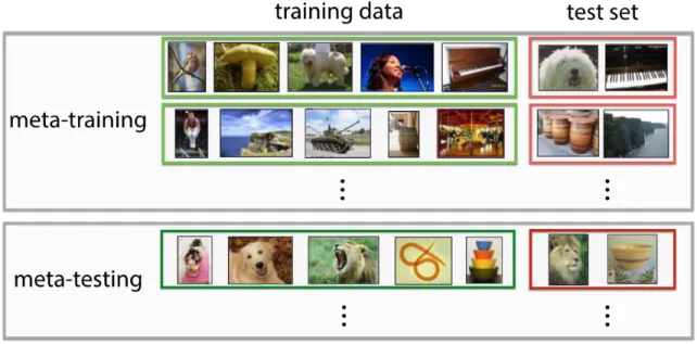
We can see this division of “meta-training” and “meta-test” in Figure 2-1, where we meta-learn across a number of few-shot classification tasks, before we are evaluated on a new set of tasks that contain classes we have not seen before during meta-training time.
Figure 2-1: Meta-training and meta-testing both contain sets of tasks to be completed, each task comprising a traditional learning problem with training and test sets. Figure from Finn’s “Learning to Learn” (2017) [7], adapted from Ravi & Larochelle (2017) [24]
.
2.4
Prior Work
Here, we describe two approaches to meta-learning in recent machine learning litera-ture: Model-Agnostic Meta-Learning and Modular Meta-Learning.
2.4.1
Model-Agnostic Meta-Learning
Model-Agnostic Meta-Learning, or MAML [8], is an algorithm used to meta-learn gradient-based learning algorithms. While the meta-learning technique is compatible with any model that can be trained through gradient descent, we still must specify the initial form of the parametric model. In particular, this paper considers deep neural networks.
Using the same framework and notation as in section 2.2, our learning algorithm 𝒜 : D × Θ → ℋ starts with a meta-learned model parametrized by 𝜃 ∈ Θ, and performs several gradient updates using the data in 𝒟 to get the final hypothesis ℎ. The outputted hypothesis has the same form as the starting meta-learned hypothesis
(just with weights altered by gradient descent), so we can summarize a hypothesis ℎ𝜃
by its corresponding parameters 𝜃 ∈ Θ. For convenience, we redefine 𝒜 : D × Θ → Θ. Additionally for convenience, let 𝒜𝜃 : D → Θ represent our learning algorithm
parametrized by starting parameters 𝜃.
The MAML algorithm consists of a nested loop, where the inner loop represents carrying out our gradient descent based adaptation algorithm 𝒜𝜃on the meta-training
tasks 𝒟(1), 𝒟(2), . . . , 𝒟(𝑁 ), while the outer loop performs the “meta-update” to our parameters 𝜃 using gradient descent to optimize the performance of 𝒜𝜃 on the
meta-training tasks. In other words, we first run the adaptation algorithm on various tasks, and then update our 𝜃 parameters using gradient descent to improve the learned hypotheses’ net performance across these tasks.
For simplicity, we assume that the adaptation algorithm consists of a single gradient step. Then, the output from applying the algorithm to task 𝑖 is 𝜃′𝑖 = 𝜃 − 𝛼∇𝜃ℒ𝒟(𝑖)
𝑡𝑟𝑎𝑖𝑛
(ℎ𝜃) for some step size 𝛼, where ℒ𝒟(ℎ𝜃) defines the loss on dataset
𝒟 for the hypothesis parameterized by 𝜃. The adapted hypothesis ℎ𝜃′𝑖 will have lower
loss on the training portion of task 𝑖, but ultimately we want it to perform well on the test portion so we do not simply learn to overfit.
Thus, we sum the performance of the adapted hypotheses on the test portion of each meta-training task, giving the following meta-objective:
min 𝜃 𝑁 ∑︁ 𝑖=1 ℒ𝒟(𝑖) 𝑡𝑒𝑠𝑡(︀ℎ𝜃 ′ 𝑖)︀ = 𝑁 ∑︁ 𝑖=1 ℒ𝒟(𝑖) 𝑡𝑒𝑠𝑡 (︂ ℎ𝜃−𝛼∇𝜃ℒ 𝒟(𝑖) 𝑡𝑟𝑎𝑖𝑛 )︂ .
As this loss is end-to-end differentiable, we can optimize it with gradient descent. The full algorithm, with computational details, can be found in the original work [8].
2.4.2
Modular Meta-Learning
Modular meta-learning [1] seeks to learn a dictionary of fixed modules that can be combined in different ways to handle different tasks. The particular manner in which the modules are combined is called its structure. Then, when presented with a new task, we simply need to search across the structure space to determine the best way
to combine the existing modules for handling this task. Here, the modules can be thought of as meta-parameters, while the search for the appropriate structure can be thought of as the adaptation step.
We begin by specifying the number of modules and their form. In the original work, these modules take the form of neural networks. Additionally, we specify how these modules can be composed (i.e. the potential structures). During the meta-training period, we provide a set of tasks and seek to learn weights for the modules such that if they are combined through the appropriate structure, they can achieve high performance on each of the tasks. As we train, we keep track of one structure for each task, which is used to produce predictions for that task. Based on the loss of these predictions, we can then compute gradient updates to the weights of the modules used for that task. Alternating with this gradient-update step is a simulated-annealing step, which searchs for better structures for each task. As the algorithm runs, we converge on the best structure for each task and the best weights for each module. Since the modules have be trained to work well to model many different tasks, we expect that these modules will be able to generalize well to new tasks too. This meta-learning algorithm is termed BounceGrad.
During the adaptation phase, we simply use simulated annealing to determine the structure that performs the best on the new task, given the modules that we have previously learned. If desired, (during both the meta-training and adaptation phase) after selecting our structure we may fine-tune our module weights using a few gradient descent steps as in MAML. This combination of modular meta-learning and MAML is referred to as MoMA.
Chapter 3
Active Learning
3.1
Description
While labelled training data can be expensive or time-consuming to collect, unlabelled data is often much more plentiful.
Active learning is an area of machine learning that hopes to make more intelligent use of labelled data. An active learning algorithm is provided with (or creates) unla-belled examples and can choose when to query the label of one of these examples. By being able to choose which specific examples to train on, the learning algorithm may be able to train a model more efficiently, leading to an equal level of performance us-ing significantly fewer labelled trainus-ing examples than would otherwise be necessary [2, 16, 4, 18].
There are three primary types of active learning: query synthesis, stream-based sampling, and pool-based sampling [27]. In query synthesis, the learner is able to construct its own unlabelled examples and then request the labels to these fabricated data points to train on. In stream-based sampling, the learner receives unlabelled data in a stream, and must decide for each point whether to query its label or to pass on it. In pool-based sampling, the learner has access to a set of unlabelled data, and can choose any example from this set to be labelled and trained on. We will primarily consider scenarios of this third type.
3.2
General Formulation
Here, we consider the basic formulation of the pool-based active learning problem. The learner is provided access to a pool 𝒰 of unlabelled data and a pool 𝒟 of labelled data, which typically starts empty. The learner can query a point from 𝒰 , receiving its label from an oracle and transferring the now labelled point to 𝒟. The learner uses the labelled points of 𝒟 (and potentially 𝒰 , in the semi-supervised setting) in order to produce a model.
But how do we evaluate the performance of an active learning algorithm? It is possible (and even likely) that the performance of the learned model is maximal after querying the label of every single data point, but this clearly defeats the purpose of active learning. One way is to plot the learning curve of the algorithm, which plots performance (e.g. accuracy) against the number of examples queried and compare it to a baseline, for example the performance of a model trained on random queries. If the learning curve appears above the the baseline curve for all numbers of queries, then the active learning algorithm seems to be effective at choosing points to train on.
Alternatively, we can view the active learning objective as minimizing the loss of the final model without exceeding some fixed annotation budget, where the learner incurs some cost each time it queries a label. Thus, the learning algorithm should hope to identify the examples or sets of examples which, if provided their labels, are likely to improve the learned model’s performance the most.
3.3
Prior Work
Here, we examine some common approaches to choosing queries during active learn-ing, as described in Settles’s active learning survey [27].
3.3.1
Uncertainty Sampling
One of the most basic active learning techniques is uncertainty sampling [18], which actively queries the point for which the current hypothesis is least confident. In this section, we describe several common formulations of uncertainty, for both classifica-tion and regression.
Classification
For classification tasks, one simple approach is least confident sampling, where we query the point ˜𝑥 whose predicted class (i.e. the class assigned the highest probability) is the smallest. For a model parametrized by 𝜃,
˜
𝑥 = arg min
𝑥
𝑝𝜃(ˆ𝑦 | 𝑥),
where ˆ𝑦 = arg max𝑦′𝑝𝜃(𝑦′ | 𝑥).
Since this technique discards all information except for the class assigned the highest probability, some people use margin sampling, which chooses the point with the smallest margin between the predicted class and the second most likely class:
˜
𝑥 = arg min
𝑥
(𝑝𝜃(ˆ𝑦1 | 𝑥) − 𝑝𝜃(ˆ𝑦2 | 𝑥)) ,
where ˆ𝑦1 and ˆ𝑦2 are the first and second most likely predicted classes.
A method that considers the entire predicted output distribution is using entropy as the uncertainty metric:
˜ 𝑥 = arg max 𝑥 −∑︁ 𝑖 𝑝𝜃(𝑦𝑖 | 𝑥) log 𝑝𝜃(𝑦𝑖 | 𝑥). Regression
Maximizing entropy under the asssumption of Gaussian distributed outputs is equiv-alent to maximizing variance. Since output variance can be estimated in many sce-narios [27], variance is a common metric of uncertainty for active learning regression
problems.
3.3.2
Query-by-Committee and Disagreement-Based Methods
The canonical query-by-committee algorithm applies to classification tasks, though extensions exist to the regression setting as well [27].
Classification
The query-by-committee algorithm [28] attempts to maximize the Shannon informa-tion of each query, using the disagreement of a committee of 𝑘 committee members in order to make its selection. Each committee member represents a model trained on the same training set. The original paper considers only the binary classification problem restricted to parametric models with continuous weights, in which the data are assumed to be perfectly separable.
In this scenario, we can view each query as reducing the size of the version space, which is the set of all weight vectors consistent with the training data. As 𝑘 goes to infinity, querying a point where half of the committee members choose a positive classification and half choose negative will bisect the version space, providing the maximum 1 bit of information per query.
More formally, assume a uniform prior over weights, such that the posterior distri-bution after some 𝑡 queries will be uniform over the version space and zero outside. If 𝑉+ represents the volume of consistent weight vectors that positively classify a query,
and 𝑉− represents the volume of those that negatively classify that query, then the information gain of the point 𝑥𝑡+1 is given by the following, where 𝑉𝑡 = 𝑉+ + 𝑉−
represents the volume of the entire version space:
𝐼𝑡+1= − 𝑉+ 𝑉𝑡 log(︂ 𝑉 + 𝑉𝑡 )︂ −𝑉 − 𝑉𝑡 log(︂ 𝑉 − 𝑉𝑡 )︂ ,
which is maximized by querying a point where 𝑉+ = 𝑉−. Of course, in practice we do not have global information of the version space, so we instead train 𝑘 models with randomly sampled weights (using Gibbs sampling) that are consistent with the
previously queried training points, and query a new data point whose classifications by the committee members are (as close as possible to) an even split.
In particular, we maximize the vote entropy, which (generalized to an arbitrary number of classes 𝑦𝑖) is given by the following [6]:
𝐼 = −∑︁ 𝑖 𝑣(𝑦𝑖) 𝑘 log (︂ 𝑣(𝑦𝑖) 𝑘 )︂ .
Here, 𝑣(𝑦𝑖) represents the number of committee members (out of a total of 𝑘) that
assign the candidate point a classification of 𝑦𝑖. While a greater 𝑘 will give a more
accurate estimate of the version space, even small committee sizes (as small as 2) appear to be effective in practice [20, 28].
Besides vote entropy, a number of other formulations of disagreement have been considered, including average KL-divergence [20] and Jensen-Shannon divergence [21].
Regression
Query-by-committee can also be adapted to regression tasks by formulating a dis-agreement metric based on the continuous output predictions of the committee mem-bers. A common measure of disagreement in this setting is simply the variance of output predictions. While this appears similar to the technique described in uncer-tainty sampling, this measure of disagreement factors in the unceruncer-tainty over both the output and the (parameters of the) models, while uncertainty sampling only considers the uncertainty of the output of a single model [27].
Extension to Self-Supervised Exploration
One recent extension of disagreement-based methods to the sample-efficient robot learning domain can be seen in Pathak et al., 2019 [23]. The particular scenario examined by this work is that of self-supervised exploration, where an agent is placed in an unfamiliar environment with no external rewards to guide the agent’s behavior. Potential goals might be for the agent to explore the environment and learn new skills in a self-supervised manner, to provide intrinsically motivated guidance when
only sparse external rewards are present, or to effectively explore and model the environment without any human intervention such that the agent is amenable to quickly learning a new task when rewards are provided.
The intrinsic reward function used to motivate the agent’s exploration in this work is a formulation of disagreement between an ensemble of models. In particular, each model in this ensemble attempts to predict the feature embedding of the next state given the current state and action to be executed, and the intrinsic reward is given by the variance of these models’ predictions. The agent is thus rewarded for taking actions for which it is less certain of what the resulting outcome will be. Once the agent has sufficiently explored some area of the environment, the models in the ensemble will converge to a similar prediction, and the agent will be discouraged from taking actions that further explore that area.
When provided with this disagreement-based intrinsic reward, an agent is able to perform well in various environments, acquiring significant external rewards in various Atari games (despite not being provided any external rewards), successfully exploring 3D Unity-based environments, and learning to interact with physical objects in a real world robot setting.
3.3.3
Variance Reduction and the Cohn Criterion
Both uncertainty sampling and disagreement based methods choose to query points whose outputs have the least confidence, but perhaps a more direct approach to optimizing our true objective is to query the point that will lead to the minimum generalization error.
Assume that the training data that we have provided our learner up to this point is given by 𝒟. Then, we would like to query the point ˜𝑥 for its label ˜𝑦 such that the model trained on 𝒟 ∪ (˜𝑥, ˜𝑦) has minimum expected loss. In general, this minimization is expensive, but we will consider the special case of regression with the objective of minimizing squared loss.
expected error of the learner is given by ∫︁
𝑥
E𝑇 [︀(ˆ𝑦(𝑥; 𝒟) − 𝑦)
2 | 𝑥]︀ 𝑝(𝑥)𝑑𝑥,
where 𝑝(𝑥) is the known prior distribution over 𝑥, and E𝑇 represents taking the
expectation over 𝑝(𝑦 | 𝑥) and datasets 𝒟.
Assume a fixed 𝑥. Then, where E[·] represents expectation over 𝑝(𝑦 | 𝑥), and E𝒟[·]
represents expectation over datasets 𝒟, we can decompose the expectation inside the integral as in Geman et al., 1992 [11]. Beginning by splitting the expectation,
E𝑇 [︀(ˆ𝑦(𝑥; 𝒟) − 𝑦)2 | 𝑥]︀ = E𝒟
[︀
E[︀(ˆ𝑦(𝑥; 𝒟) − 𝑦)2 | 𝑥]︀]︀ ,
we will first consider the argument to the outer expectation and perform the bias-variance decomposition with respect to 𝑝(𝑦 | 𝑥):
E[︀(ˆ𝑦(𝑥; 𝒟) − 𝑦)2 | 𝑥]︀ = E [︀((ˆ𝑦(𝑥; 𝒟) − E[𝑦 | 𝑥]) + (E[𝑦 | 𝑥] − 𝑦))2 | 𝑥]︀ = E[︀(ˆ𝑦(𝑥; 𝒟) − E[𝑦 | 𝑥])2 | 𝑥]︀ + E [︀(E[𝑦 | 𝑥] − 𝑦)2 | 𝑥]︀ + 2 E [(ˆ𝑦(𝑥; 𝒟) − E[𝑦 | 𝑥]) (E[𝑦 | 𝑥] − 𝑦) | 𝑥] = (ˆ𝑦(𝑥; 𝒟) − E[𝑦 | 𝑥])2+ E[︀(E[𝑦 | 𝑥] − 𝑦)2 | 𝑥]︀ + 2 (ˆ𝑦(𝑥; 𝒟) − E[𝑦 | 𝑥]) E [(E[𝑦 | 𝑥] − 𝑦) | 𝑥] = (ˆ𝑦(𝑥; 𝒟) − E[𝑦 | 𝑥])2+ E[︀(E[𝑦 | 𝑥] − 𝑦)2 | 𝑥]︀
+ 2 (ˆ𝑦(𝑥; 𝒟) − E[𝑦 | 𝑥]) (E[𝑦 | 𝑥] − E[𝑦 | 𝑥]) = (ˆ𝑦(𝑥; 𝒟) − E[𝑦 | 𝑥])2+ E[︀(E[𝑦 | 𝑥] − 𝑦)2 | 𝑥]︀ . Now applying the outer expectation, we have
E𝑇 [︀(ˆ𝑦(𝑥; 𝒟) − 𝑦)2 | 𝑥]︀ = E𝒟[︀(ˆ𝑦(𝑥; 𝒟) − E[𝑦 | 𝑥])2+ E[︀(E[𝑦 | 𝑥] − 𝑦)2 | 𝑥
]︀]︀
= E𝒟[︀(ˆ𝑦(𝑥; 𝒟) − E[𝑦 | 𝑥])2]︀ + E [︀(E[𝑦 | 𝑥] − 𝑦)2 | 𝑥
]︀
distribution 𝑝(𝑥, 𝑦) and out of our control. So, we consider the first term and perform another bias-variance decomposition, this time with respect to datasets 𝒟:
E𝒟[︀(ˆ𝑦(𝑥; 𝒟) − E[𝑦 | 𝑥])2]︀ = E𝒟[︀((ˆ𝑦(𝑥; 𝒟) − E𝒟[ˆ𝑦(𝑥; 𝒟)]) + (E𝒟[ˆ𝑦(𝑥; 𝒟)] − E[𝑦 | 𝑥]))2 ]︀ = E𝒟[︀(ˆ𝑦(𝑥; 𝒟) − E𝒟[ˆ𝑦(𝑥; 𝒟)])2 ]︀ + E𝒟[︀(E𝒟[ˆ𝑦(𝑥; 𝒟)] − E[𝑦 | 𝑥])2 ]︀ + 2 E𝒟[(ˆ𝑦(𝑥; 𝒟) − E𝒟[ˆ𝑦(𝑥; 𝒟)]) (E𝒟[ˆ𝑦(𝑥; 𝒟)] − E[𝑦 | 𝑥])] = E𝒟[︀(ˆ𝑦(𝑥; 𝒟) − E𝒟[ˆ𝑦(𝑥; 𝒟)])2]︀ + (E𝒟[ˆ𝑦(𝑥; 𝒟)] − E[𝑦 | 𝑥])2 + 2 (E𝒟[ˆ𝑦(𝑥; 𝒟)] − E𝒟[ˆ𝑦(𝑥; 𝒟)]) (E𝒟[ˆ𝑦(𝑥; 𝒟)] − E[𝑦 | 𝑥]) = E𝒟[︀(ˆ𝑦(𝑥; 𝒟) − E𝒟[ˆ𝑦(𝑥; 𝒟)])2]︀ + (E𝒟[ˆ𝑦(𝑥; 𝒟)] − E[𝑦 | 𝑥])2
Here, the second term represents the squared bias of the learner. If we assume that the learners we consider are unbiased, then minimizing generalization error is equivalent to minimizing the learner’s variance. In other words, we should query the point such that adding it to our training set leads to minimum posterior variance.
The work by Cohn et al., 1996 [5] derives closed form estimates for posterior vari-ance in neural networks, Gaussian mixture models, and locally weighted regression. We refer to the value of the posterior variance as the Cohn criterion for selecting query points.
Chapter 4
Joining Meta-Learning and Active
Learning
4.1
Prior Work
In this section, we examine two works that build upon Model-Agnostic Meta-Learning [8] (discussed in 2.4.1): Bayesian Model-Agnostic Meta-Learning and Probabilistic Model-Agnostic Meta-Learning. Both extensions to MAML recognize the importance of modelling the uncertainty and ambiguity inherent when learning new tasks from few data points. Being able to capture this uncertainty provides for the opportunity to perform active learning during the adaptation step at meta-test time.
4.1.1
Bayesian Model-Agnostic Meta-Learning
Bayesian MAML [14] seeks to model a posterior distribution for examples of a given task, unlike traditional MAML that provides only a point estimate. The work pro-poses two Bayesian ensemble methods that can serve this purpose, Bayesian Fast Adaptation and Bayesian Meta-Learning, of which the latter attempts to improve upon shortcomings of the former. We first begin with some preliminaries.
Stein Variational Gradient Descent
Stein Variational Gradient Descent, or SVGD, is a variational inference method that leverages gradient descent to learn a target distribution [19]. In particular, we main-tain a set of 𝑘 particles Θ = {𝜃(𝑖)}𝑘
𝑖=1 that will serve to approximate the target
distribution 𝑝(𝜃). We learn these particles by using the following update rule:
𝜃(𝑡+1) ← 𝜃(𝑡) + 𝜖(𝑡)𝜑(𝜃(𝑡)), where 𝜑(𝜃(𝑡)) = 1 𝑘 𝑘 ∑︁ 𝑗=1 [︁ 𝑘(𝜃𝑗(𝑡), 𝜃(𝑡))∇𝜃(𝑡) 𝑗 log 𝑝(𝜃(𝑡)𝑗 ) + ∇𝜃(𝑡) 𝑗 𝑘(𝜃𝑗(𝑡), 𝜃(𝑡))]︁.
Here, 𝜖(𝑡) is the step size, and 𝑘(·, ·) is a positive-definite kernel. The first term updates the particle based on a smoothed gradient that is the weighted sum of particle gradients weighted by kernel distance. The second term provides a repulsive force that prevents the particles from collapsing to local modes.
Bayesian Fast Adaptation
We begin with the probabilistic interpretation of MAML, which is to determine meta-parameters 𝜃 to maximize the following objective, given meta-training set D𝑡𝑟𝑎𝑖𝑛 =
{𝒟(1), 𝒟(2), . . . , 𝒟(𝑛)}: 𝐽 (𝜃) = 𝑛 ∏︁ 𝑖=1 𝑝(︁𝒟(𝑖)𝑡𝑒𝑠𝑡 | 𝜃(𝑖)′ = 𝜃 − 𝛼∇ 𝜃log 𝑝(𝒟 (𝑖) 𝑡𝑟𝑎𝑖𝑛 | 𝜃) )︁ (4.1)
We extend this objective in the form of a hierarchical Bayesian model [12],
𝐽 (𝜃) = 𝑛 ∏︁ 𝑖=1 ∫︁ 𝑝(︁𝒟(𝑖)𝑡𝑒𝑠𝑡 | 𝜃(𝑖))︁𝑝(𝜃(𝑖) | 𝒟(𝑖) 𝑡𝑟𝑎𝑖𝑛, 𝜃)𝑑𝜃 (𝑖) ≈ 𝑛 ∏︁ 𝑖=1 1 𝑘 𝑘 ∑︁ 𝑗=1 𝑝(︁𝒟(𝑖)𝑡𝑒𝑠𝑡| 𝜃𝑗(𝑖))︁, (4.2) for 𝜃(𝑖)𝑗 ∼ 𝑝(𝜃(𝑖) | 𝒟(𝑖) 𝑡𝑟𝑎𝑖𝑛, 𝜃).
We see that the first objective is a special case of the second, where the posterior of adapted parameters 𝑝(𝜃(𝑖) | 𝒟(𝑖)
𝑡𝑟𝑎𝑖𝑛) is approximated by the single point estimate 𝜃(𝑖)′,
which can be interpreted as the maximum a posteriori (MAP) estimate for 𝜃(𝑖) [12]. To provide greater flexibility, instead of a point estimate we will maintain a series of par-ticles Θ = {𝜃(1), . . . , 𝜃(𝑘)} such that, after running SVGD, they appropriately model
the posterior. In other words, while MAML involves finding the meta-parameters 𝜃 that can quickly be adapted to the MAP estimate using gradient descent, now we seek meta-parameters Θ that can quickly be adapted to approximating the entire posterior distribution using SVGD.
We will set our target distribution for SVGD to be
𝑝(𝜃(𝑖) | 𝒟(𝑖)𝑡𝑟𝑎𝑖𝑛) ∝ 𝑝(𝒟(𝑖)𝑡𝑟𝑎𝑖𝑛 | 𝜃(𝑖))𝑝(𝜃(𝑖)).
The data likelihood is assumed to be Gaussian, and the second term 𝑝(𝜃(𝑖)) is the prior over parameters weights, and is chosen by us. We take Θ(𝑖) = 𝑆𝑉 𝐺𝐷
𝑡(Θ, 𝒟 (𝑖) 𝑡𝑟𝑎𝑖𝑛)
be the task-specific particles resulting from applying SVGD for 𝑡 steps on particles initialized to Θ. Then, taking the log of our approximate objective in 4.2 gives us a meta-loss function ℒ𝐵𝐹 𝐴 = 𝑛 ∑︁ 𝑖=1 log [︃ 1 𝑘 𝑘 ∑︁ 𝑗=1 𝑝 (︁ 𝒟(𝑖)𝑡𝑒𝑠𝑡 | 𝜃(𝑖)𝑗 )︁ ]︃ ,
which we can use to train our meta-parameters Θ with gradient descent.
While Bayesian Fast Adaptation extends MAML to allow for Bayesian inference, it can still overfit to the meta-training tasks. Only the inner loop adaptation steps actually make use of a Bayesian framework through SVGD; the meta-learning update step simply minimizes empirical loss summed across the meta-training tasks and thus may not properly model uncertainty over the true distribution of tasks.
Bayesian Meta-Learning with Chaser Loss
The authors tackle this issue by formulating a new objective: to minimize the dis-tance of the task-specific posterior distributions from the true posteriors. Our ap-proximation of the posterior for task 𝑖 is given by Θ(𝑖)𝑡 = 𝑆𝑉 𝐺𝐷𝑡(Θ, 𝒟
(𝑖)
𝑡𝑟𝑎𝑖𝑛), while we
approximate the true posterior by running additional SVGD steps after augmenting the dataset with the remaining data of the task: Θ(𝑖)𝑡+𝑠 = 𝑆𝑉 𝐺𝐷𝑠(Θ
(𝑖) 𝑡 , 𝒟 (𝑖) 𝑡𝑟𝑎𝑖𝑛∪ 𝒟 (𝑖) 𝑡𝑒𝑠𝑡).
Θ(𝑖)𝑡 is considered the chaser, while Θ(𝑖)𝑡+𝑠 is the leader, and during meta-training we would like to find the initialization Θ that allows the chaser to catch the leader.
Our meta-loss function becomes the following:
ℒ𝐵𝑀 𝐴𝑀 𝐿 = 𝑛
∑︁
𝑖=1
𝑑(Θ(𝑖)𝑡 , Θ(𝑖)𝑡+𝑠),
where 𝑑(·, ·) is a distance metric, which in this case has chosen to be the summed Euclidean distance between paired particles. Note that the gradients should not propogate through the leader, which are treated to represent the true targets. The full algorithm can be found in the original work [14].
Active Learning
This ability to model a posterior distribution captures uncertainty in predictions and gives the chance to perform active learning during the adaptation phase. Assume we have some (potentially empty) set of labelled data 𝒟 for our task 𝑖, from which we can obtain the task-specific particles Θ(𝑖), along with a set of unlabelled data 𝒰 .
The authors consider active learning in the classification setting, where the particles provide us with an estimate of 𝑝(𝑦 | 𝑥, 𝒟). Then, we simply query the point with maximum entropy: 𝑥* = arg max 𝑥∈𝒰 H[𝑦 | 𝑥, 𝒟] = − ∑︁ 𝑦′ 𝑝(𝑦′ | 𝑥, 𝒟) log 𝑝(𝑦′ | 𝑥, 𝒟).
After obtaining the label 𝑦* for this example, we remove it from 𝒰 add it to 𝒟, perform the adaptation step again, and repeat.
4.1.2
Probabilistic Model-Agnostic Meta-Learning
Probabilistic Model-Agnostic Meta-Learning [10] also extends conventional MAML into a hierarchical Bayesian model, modelling the prior distribution of meta-parameters 𝜃 and predicting a posterior distribution over adapted parameters 𝜑𝑖 (analogous to
the 𝜃𝑖′ in conventional MAML) by conditioning on the task-specific data points in 𝒟(𝑖).
The prior over meta-parameters 𝑝(𝜃) is chosen to be Gaussian, with a learned mean and learned diagonal covariance. We next decide how to treat the prior 𝑝(𝜑𝑖 |
𝜃). Using the probabilistic interpretation of MAML [12], MAML’s gradient descent updates using training examples 𝒟(𝑖)𝑡𝑟𝑎𝑖𝑛 can be viewed as MAP inference of 𝜑𝑖 given
𝒟(𝑖)𝑡𝑟𝑎𝑖𝑛, assuming a Gaussian prior 𝑝(𝜑𝑖 | 𝜃) and Gaussian likelihood 𝑝(𝒟(𝑖) | 𝜑𝑖, 𝜃) =
𝑝(𝒟(𝑖)𝑡𝑟𝑎𝑖𝑛 | 𝜑𝑖). Rather than using an explicit Gaussian prior, the implicit prior appears
to exhibit good performance in practice [8, 12]. Thus, we use gradient descent updates with training data 𝒟(𝑖)𝑡𝑟𝑎𝑖𝑛 on starting parameters 𝜃 to obtain 𝜑*𝑖. This point estimate approximates the posterior 𝑝(𝜑𝑖 | 𝒟
(𝑖)
𝑡𝑟𝑎𝑖𝑛, 𝜃), and implies our prior for 𝑝(𝜑𝑖 | 𝜃).
The challenge of optimizing the meta-parameters given non-deterministic 𝜃 can be handled with structured variational inference, with the details described in the original work [10]. The final adaptation algorithm at meta-test time appears very similar to the original adaptation method in MAML; however, we have one additional step of sampling 𝜃 from the meta-learned prior 𝑝(𝜃) before performing the standard MAML adaptation using the task’s training data.
Active Learning
While the original authors do not investigate the application of active learning to Probabilistic MAML, we can envision performing active learning in a similar way as in Bayesian MAML. Probabilistic MAML provides us with a distribution of models from which we can sample. So, for a task with labelled data 𝒟 and unlabelled data 𝒰 , for each candidate 𝑥 ∈ 𝒰 we gain the ability to sample from the posterior distribution over predicted labels. We can then estimate the uncertainty in the predictions, for
example by computing the variance or the entropy (for classification problems) of the sampled labels.
4.2
Our Method: Modular Meta-Learning
In our work, we use the modular meta-learning framework [1] as described in section 2.4.2. After the meta-training phase, we obtain a set of trained modules; during adaptation to a new task, we search across the structure space to determine the best performing structure.
For the purpose of active learning, assume the current set of labelled examples is 𝒟, and the finite set of unlabelled examples is 𝒰 . Let 𝒮 be an arbitrary structure. For a uniform prior over structures,
𝑝(𝒮 | 𝒟) ∝ 𝑝(𝒟 | 𝒮) · 𝑝(𝒮) ∝ 𝑝(𝒟 | 𝒮).
In our experiments, we will consider working with the quadratic loss function. If we assume our training set residuals are i.i.d. Gaussian random variables, then if 𝑆𝑆𝐸𝒮
corresponds to the sum of squared errors for structure 𝒮,
𝑝(𝒮 | 𝒟) ∝ 𝑝(𝒟 | 𝒮) ∝ 1 (2𝜋𝜎2)‖𝒟‖/2𝑒 −𝑆𝑆𝐸𝒮 2𝜎2 ∝ 𝑒−𝑆𝑆𝐸𝒮2𝜎2 ,
where 𝜎2 represents the variance of the noise in the data. We can estimate the value
of 𝜎2 from the mean squared error of the best structure for tasks in the meta-training set; for active learning purposes, the accuracy of this value will not be crucial, as estimating it to the right order of magnitude works well empirically.
Computing the sum of squared errors for potential structures thus gives us a posterior distribution over the structures. We consider three different active learning criteria that we can compute using this distribution: variance, entropy, and the Cohn
criterion.
Variance
The first criterion we consider is variance, which we use to choose our query point ˜𝑥 as follows:
˜
𝑥𝑣𝑎𝑟 = arg max 𝑥∈𝒰
Var[𝑦 | 𝑥, 𝒟]
In particular, for a given candidate 𝑥 we would like to determine the variance of its label, which is given by the random variable
𝑌 ∼ 𝑝(𝑦 | 𝑥, 𝒟) =∑︁
𝒮
𝑝(𝑦 | 𝑥, 𝒟, 𝒮) · 𝑝(𝒮 | 𝑥, 𝒟) = ∑︁
𝒮
𝑝(𝑦 | 𝑥, 𝒮) · 𝑝(𝒮 | 𝒟).
We can thus estimate this variance by sampling structures, computing the predicted labels for 𝑥 given these structures, and taking the variance of these labels.
Entropy
The second criterion is entropy, in particular the entropy of the posterior distribution over structures given the point 𝑥 and its label:
˜
𝑥𝑒𝑛𝑡 = arg max
𝑥∈𝒰 H[𝑆 | 𝒟 ∪(𝑥, 𝑦)]
Here, we simply determine the posterior distribution 𝑝(𝒮 | 𝒟 ∪(𝑥, 𝑦)) by augmenting our dataset with the newly queried point and computing the posterior distribution in the same manner we initially computed 𝑝(𝒮 | 𝒟).
In practice, we sample a structure, compute the predicted label for candidate 𝑥, and add the candidate and label to the training set. We then recompute the sum of squared errors for each structure, which allows us to obtain an updated distribution over the structures, and compute the entropy over this distribution. Repeating the sampling process and taking the mean over the resulting entropies gives us a final estimate for this criterion.
Cohn Criterion
Finally, we examine the Cohn criterion, whose value we will negate since it is desirable to query the point that leads to the smallest value of the Cohn criterion. Specifically, we query ˜ 𝑥𝑐𝑜ℎ𝑛= arg max 𝑥∈𝒰 − ∫︁ 𝑥′ Var [𝑦′ | 𝑥′, 𝒟 ∪(𝑥, 𝑦)] 𝑝(𝑥′)𝑑𝑥′, where 𝑦′ is the label of 𝑥′.
We begin by sampling a structure and using the same process as for entropy to obtain an updated distribution over the structures. Then, we use this updated distribution to compute the output variance, integrated over the input domain. In practice, we assume a uniform input distribution 𝑝(𝑥′) and estimate the integral by sampling from the domain of 𝑥′. Repeating and averaging this process over multiple samplings of the structure gives us an estimate for the Cohn criterion.
For any of the criteria, active learning proceeds as follows. Compute the criterion value for each candidate 𝑥 ∈ 𝒰 and choose the candidate ˜𝑥 with the largest value. Query its label ˜𝑦, removing ˜𝑥 from 𝒰 and adding (˜𝑥, ˜𝑦) to the dataset 𝒟. Finally, retrain and repeat.
Chapter 5
Experiments and Results
5.1
Alet Function Regression
The following dataset of summed functions was first introduced by Alet et al. [1] alongside the Modular Meta-Learning technique.
5.1.1
Summed Function Regression Problem
The tasks within this meta-learning problem are 1D regression problems in which each task corresponds the sum of two common nonlinear functions, such as 𝑓 (𝑥) = sin(𝑥) or 𝑓 (𝑥) = ⌊𝑥⌋, over the domain [−1, 1]. A new task consists of a pair of these basis functions whose combination has not been seen before, where the challenge is to properly model the sum of the functions given just a small number of examples.
There are a total of 16 distinct functions, leading to a total of 256 distinct potential tasks; 230 are used during for training, and the remainder are used for meta-testing [1]. During the adaptation phase, we start with no labelled data and have a pool of 32 unlabelled candidates to choose from.
Methods and Results
We first build up the modules needed to adapt to new tasks. All modules are feed-forward neural networks, 10 with a single hidden layer of 16 units and 10 with two
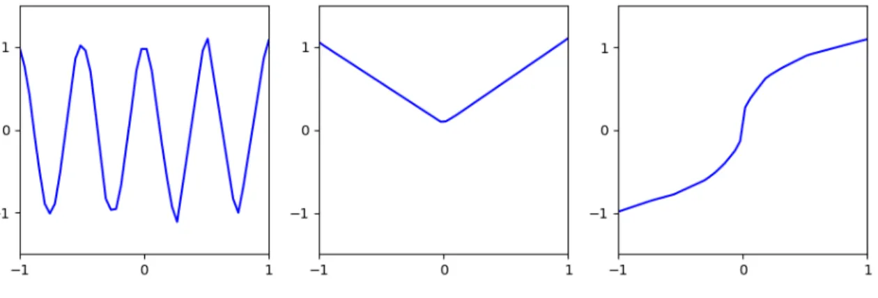
hidden layers each with 16 units. We compose pairs of modules by simply summing their outputs. After running the BounceGrad algorithm, we can visually ascertain that many of the modules have learned to capture individual basis functions, and that they can successfully fit the meta-training tasks.
Figure 5-1: Sample modules after the meta-training phase.
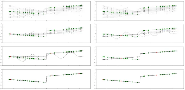
Next, we evaluate the performance of active learning during the adaptation phase, comparing the effectiveness of queries based on variance, entropy, and the Cohn crite-rion to random queries. We visualize an example task and the first few points queried using variance and the Cohn criterion in Figure 5-2 below, showing how the distribu-tion over structures changes with each query. The green points are candidate points in the unlabelled pool of data; the red points are points that have been queried. We can see that the two methods choose different points to query. Nonetheless in both cases, starting with a uniform distribution over possible structures, the algorithm quickly converges to a structure that suits the task very well.
Computing the mean squared error across various numbers of queries for many tasks, we find that actively querying points does seem to confer significant benefits over random queries for the first few queries (i.e. before convergence). These error values can be found in Table 5.1. It is less clear which specific active learning technique is superior. We additionally visualize the mean squared error against queries in Figure 5-3, showing that the entropy and Cohn criteria effectively reach convergence after four queries, while random queries take several more training points.
Figure 5-2: A visualization of the initial prior (uniform) distribution over structures, and the posterior distributions, as an active learner queries new points (in red) using variance (left) and the Cohn criterion (right). Darker lines correspond to structures assigned higher probabilities.
Number of Queries Criterion 0 1 2 3 4 Random 50.9 28.6 12.6 7.05 3.49 Variance 51.1 21.7 10.4 2.53 1.15 Entropy 50.9 25.1 9.17 0.409 0.273 Cohn 51.1 19.6 8.10 1.15 0.291
Table 5.1: Mean squared error (×10−2) for random queries and different active learn-ing criteria in the Alet function dataset. Numbers in bold are not significantly differ-ent from the best technique for that number of queries.
Figure 5-3: A plot of mean squared error by number of queries for the Alet function dataset, with error bars of 1 standard deviation.
5.2
Omnipush Dataset
5.2.1
Dataset Description
The Omnipush dataset is a collection of pushing dynamics of 250 different shaped ob-jects. In particular, the dataset contains 250 random pushes of each object, recording the starting and ending states (position and orientation) of the object. Details on the data collection technique can be found in [3].
Each object is formed from a central piece with four modular attachments, which can be either concave, rectangular, triangular, or circular. In addition, extra weights (light or heavy) can be placed on the attachments in order to alter the mass distri-bution of the object.
5.2.2
Meta-Learning Problem
Here, each task consists of the pushes corresponding to a single object. Thus, the challenge of a new task is to model the pushing dynamics of the object given just a
Figure 5-4: An example Omnipush object displaying the four different attachments and an extra weight. Figure from Bauza et al. (2018) [3]
few example pushes. During the adaptation phase, we have a pool of 80 unlabelled candidates to choose from.
Methods and Results
As in Section 5.1.1, we first train our modules using the BounceGrad algorithm. We use 12 modules in total, where 6 have a single hidden layer of 12 units and 6 have two hidden layers of 6 units each.
We next evaluate the performance of active learning during the adaptation phase, testing variance, entropy, and the Cohn criterion for active learning as compared to random query baselines.
We compute the mean squared error across various numbers of queries, and again find that actively querying points does seem to confer significant benefits over random queries prior to convergence. These error values can be found in Table 5.2.
Number of Queries Criterion 0 1 2 3 4 5 Random 0.203 0.196 0.191 0.187 0.184 0.182 Variance 0.204 0.197 0.189 0.185 0.180 0.175 Entropy 0.203 0.189 0.181 0.177 0.172 0.167 Cohn 0.203 0.188 0.183 0.177 0.173 0.169
Table 5.2: Mean squared error for random queries and different active learning criteria for the Omnipush dataset. Numbers in bold are not significantly different from the best technique for that number of queries.
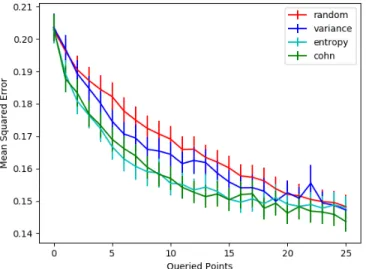
We plot the mean squared error values against number of queries in Figure 5-5. All three methods of active learning appear to exhibit advantages over random queries, though using entropy and the Cohn criterion appear superior to actively querying based on variance.
Figure 5-5: A plot of mean squared error by number of queries for the Omnipush dataset, with error bars of 1 standard deviation.
Visualizing the pushes being chosen by the various active learning criteria, we notice that, qualitatively, the variance criterion more often tends to query pushes that are nearby one another, while the other two generally choose pushes that are further spread apart. It appears that entropy and the Cohn criterion, which are more closely aligned with our goals in active learning (trying to gain information on the correct structure and minimizing posterior loss, respectively), may be less susceptible to simply querying regions of higher variance.
An example of the active learning queries made by the three criteria on an Om-nipush example is presented below.
Figure 5-6: A display of the first 8 pushes (in black) queried by the variance (top left), entropy (top right), and Cohn (bottom) active learning criteria for an Omnipush example.
Chapter 6
Conclusion
Deep learning and the rise of “big data” have led to innumerable advances in recent years across a range of fields and broad spectrum of applications. However, the availability of “big data” is not always a given. In certain applications, including but by no means limited to robotics, acquiring labelled data can be expensive and time-consuming. Independent of the issue of data collection, in some scenarios we desire to be quickly adaptable to new tasks, which means training on large datasets is computationally infeasible.
We investigated the combination of meta-learning and active learning techniques, both of which exhibit promise for learning more quickly and from less data. In order to perform active learning in conjunction with meta-learning, we need some method to rank candidate examples to decide which are likely to be the most informative. These methods often take the form of some “uncertainty” metric, where the learner is able to gauge its own uncertainty in a predicting a given example. The meta-learning techniques Bayesian MAML [14] and Probabilistic MAML [10] reformulate MAML [8] as hierarchical Bayesian models, allowing them to predict distributions of labels and thus giving a metric of uncertainty for any input.
Instead, in this paper we show how to use the Modular Meta-Learning framework [1] with active learning; the structures implicity define a distribution over outputs, which can also be used to compute uncertainty metrics or values such as the Cohn criterion for active learning. We test this combination of active learning and
meta-learning in two different scenarios, the summed functions dataset introduced by Alet et al. [1] and the Omnipush dataset [3]. In both, we find that active learning displays significant advantages over random queries, showing promise for the combination of meta-learning and active learning in further reducing data needs.
Bibliography
[1] Ferran Alet, Tomas Lozano-Perez, and Leslie P. Kaelbling. Modular meta-learning. In Aude Billard, Anca Dragan, Jan Peters, and Jun Morimoto, editors, Proceedings of The 2nd Conference on Robot Learning, volume 87 of Proceedings of Machine Learning Research, pages 856–868. PMLR, 29–31 Oct 2018.
[2] Dana Angluin. Queries and concept learning. Machine learning, 2(4):319–342, 1988.
[3] Maria Bauza, Ferran Alet, Yen-Chen Lin, Tomás Lozano-Pérez, Leslie P. Kael-bling, Phillip Isola, and Alberto Rodriguez. Omnipush: accurate, diverse, real-world dataset of pushing dynamics with rgbd images. 2018.
[4] David Cohn, Les Atlas, and Richard Ladner. Improving generalization with active learning. Machine learning, 15(2):201–221, 1994.
[5] David A Cohn, Zoubin Ghahramani, and Michael I Jordan. Active learning with statistical models. Journal of artificial intelligence research, 4:129–145, 1996. [6] Ido Dagan and Sean P Engelson. Committee-based sampling for training
prob-abilistic classifiers. In Machine Learning Proceedings 1995, pages 150–157. Else-vier, 1995.
[7] Chelsea Finn. Learning to learn, Jul 2017.
[8] Chelsea Finn, Pieter Abbeel, and Sergey Levine. Model-agnostic meta-learning for fast adaptation of deep networks. CoRR, abs/1703.03400, 2017.
[9] Chelsea Finn and Sergey Levine. Meta-learning: from few-shot learning to rapid reinforcement learning, Jun 2019.
[10] Chelsea Finn, Kelvin Xu, and Sergey Levine. Probabilistic model-agnostic meta-learning. In Advances in Neural Information Processing Systems, pages 9516– 9527, 2018.
[11] Stuart Geman, Elie Bienenstock, and René Doursat. Neural networks and the bias/variance dilemma. Neural computation, 4(1):1–58, 1992.
[12] Erin Grant, Chelsea Finn, Sergey Levine, Trevor Darrell, and Thomas Griffiths. Recasting gradient-based meta-learning as hierarchical bayes. arXiv preprint arXiv:1801.08930, 2018.
[13] Norman P Jouppi, Cliff Young, Nishant Patil, David Patterson, Gaurav Agrawal, Raminder Bajwa, Sarah Bates, Suresh Bhatia, Nan Boden, Al Borchers, et al. In-datacenter performance analysis of a tensor processing unit. In 2017 ACM/IEEE 44th Annual International Symposium on Computer Architecture (ISCA), pages 1–12. IEEE, 2017.
[14] Taesup Kim, Jaesik Yoon, Ousmane Dia, Sungwoong Kim, Yoshua Bengio, and Sungjin Ahn. Bayesian model-agnostic meta-learning. arXiv preprint arXiv:1806.03836, 2018.
[15] Alex Krizhevsky, Ilya Sutskever, and Geoffrey E Hinton. Imagenet classification with deep convolutional neural networks. In Advances in neural information processing systems, pages 1097–1105, 2012.
[16] Ken Lang. Newsweeder: Learning to filter netnews. In Machine Learning Pro-ceedings 1995, pages 331–339. Elsevier, 1995.
[17] Christiane Lemke, Marcin Budka, and Bogdan Gabrys. Metalearning: a survey of trends and technologies. Artificial intelligence review, 44(1):117–130, 2015. [18] David D Lewis and William A Gale. A sequential algorithm for training text
classifiers. In SIGIR’94, pages 3–12. Springer, 1994.
[19] Qiang Liu and Dilin Wang. Stein variational gradient descent: A general pur-pose bayesian inference algorithm. In Advances in neural information processing systems, pages 2378–2386, 2016.
[20] Andrew Kachites McCallumzy and Kamal Nigamy. Employing em and pool-based active learning for text classification. Citeseer.
[21] Prem Melville, Stewart M Yang, Maytal Saar-Tsechansky, and Raymond Mooney. Active learning for probability estimation using jensen-shannon di-vergence. In European conference on machine learning, pages 268–279. Springer, 2005.
[22] D.K. Naik and R.J. Mammone. Meta-neural networks that learn by learning. [Proceedings 1992] IJCNN International Joint Conference on Neural Networks. [23] Deepak Pathak, Dhiraj Gandhi, and Abhinav Gupta. Self-supervised exploration
via disagreement. CoRR, abs/1906.04161, 2019.
[24] Sachin Ravi and Hugo Larochelle. Optimization as a model for few-shot learning. In ICLR, 2017.
[25] Albert Reuther, Jeremy Kepner, Chansup Byun, Siddharth Samsi, William Ar-cand, David Bestor, Bill Bergeron, Vijay Gadepally, Michael Houle, Matthew Hubbell, et al. Interactive supercomputing on 40,000 cores for machine learning and data analysis. In 2018 IEEE High Performance extreme Computing Confer-ence (HPEC), pages 1–6. IEEE, 2018.
[26] Jürgen Schmidhuber. Evolutionary principles in self-referential learning, or on learning how to learn: the meta-meta-... hook. PhD thesis, Technische Universität München, 1987.
[27] Burr Settles. Active learning literature survey. Computer Sciences Technical Report 1648, University of Wisconsin–Madison, 2009.
[28] H. S. Seung, M. Opper, and H. Sompolinsky. Query by committee. In Proceedings of the Fifth Annual Workshop on Computational Learning Theory, COLT ’92, pages 287–294, New York, NY, USA, 1992. ACM.
[29] David Silver, Aja Huang, Chris J Maddison, Arthur Guez, Laurent Sifre, George Van Den Driessche, Julian Schrittwieser, Ioannis Antonoglou, Veda Panneershel-vam, Marc Lanctot, et al. Mastering the game of go with deep neural networks and tree search. nature, 529(7587):484, 2016.