HAL Id: hal-02658867
https://hal.inrae.fr/hal-02658867
Submitted on 30 May 2020
HAL is a multi-disciplinary open access
archive for the deposit and dissemination of
sci-entific research documents, whether they are
pub-lished or not. The documents may come from
teaching and research institutions in France or
abroad, or from public or private research centers.
L’archive ouverte pluridisciplinaire HAL, est
destinée au dépôt et à la diffusion de documents
scientifiques de niveau recherche, publiés ou non,
émanant des établissements d’enseignement et de
recherche français ou étrangers, des laboratoires
publics ou privés.
software DIYABC (v1.0)
Jean-Marie Cornuet, Virginie Ravigné, Arnaud Estoup
To cite this version:
Jean-Marie Cornuet, Virginie Ravigné, Arnaud Estoup. Inference on population history and model
checking using DNA sequence and microsatellite data with the software DIYABC (v1.0). BMC
Bioin-formatics, BioMed Central, 2010, 11, pp.401. �10.1186/1471-2105-11-401�. �hal-02658867�
R E S E A R C H A R T I C L E
Open Access
Inference on population history and model
checking using DNA sequence and microsatellite
data with the software DIYABC (v1.0)
Jean-Marie Cornuet
1, Virgine Ravigné
2, Arnaud Estoup
1*Abstract
Background: Approximate Bayesian computation (ABC) is a recent flexible class of Monte-Carlo algorithms increasingly used to make model-based inference on complex evolutionary scenarios that have acted on natural populations. The software DIYABC offers a user-friendly interface allowing non-expert users to consider population histories involving any combination of population divergences, admixtures and population size changes. We here describe and illustrate new developments of this software that mainly include (i) inference from DNA sequence data in addition or separately to microsatellite data, (ii) the possibility to analyze five categories of loci considering balanced or non balanced sex ratios: autosomal diploid, autosomal haploid, X-linked, Y-linked and mitochondrial, and (iii) the possibility to perform model checking computation to assess the“goodness-of-fit” of a model, a feature of ABC analysis that has been so far neglected.
Results: We used controlled simulated data sets generated under evolutionary scenarios involving various
divergence and admixture events to evaluate the effect of mixing autosomal microsatellite, mtDNA and/or nuclear autosomal DNA sequence data on inferences. This evaluation included the comparison of competing scenarios and the quantification of their relative support, and the estimation of parameter posterior distributions under a given scenario. We also considered a set of scenarios often compared when making ABC inferences on the routes of introduction of invasive species to illustrate the interest of the new model checking option of DIYABC to assess model misfit.
Conclusions: Our new developments of the integrated software DIYABC should be particularly useful to make inference on complex evolutionary scenarios involving both recent and ancient historical events and using various types of molecular markers in diploid or haploid organisms. They offer a handy way for non-expert users to achieve model checking computation within an ABC framework, hence filling up a gap of ABC analysis. The software DIYABC V1.0 is freely available at http://www1.montpellier.inra.fr/CBGP/diyabc.
Background
Natural populations are often characterized by complex demographic histories. Their effective sizes and ranges change over time leading to fission and fusion processes that leave signatures on their genetic constitution and structure. One promising prospect of current biology is that molecular data will help us to reveal the complex demographic processes that have acted on populations. The extensive availability of different molecular markers
and increased computer power has promoted the devel-opment of inferential methods and associated software that have begun to fulfil these expectations [1,2].
Approximate Bayesian computation (ABC) is a recent flexible class of Monte-Carlo algorithms for performing model-based inference [3]. Estimations associated with demographic and genetic models often imply a full like-lihood calculation, which is difficult for complex evolu-tionary scenarios. ABC methods bypass exact likelihood calculations by using summary statistics and massive computer simulations and make it possible to handle large data sets, such as data for hundreds of individuals genotyped at tens of microsatellite loci. The
* Correspondence: [email protected] 1
INRA, UMR CBGP (INRA/IRD/Cirad/Montpellier SupAgro), Campus international de Baillarguet, CS 30016, F-34988 Montferrier-sur-Lez cedex, France
© 2010 Cornuet et al; licensee BioMed Central Ltd. This is an Open Access article distributed under the terms of the Creative Commons Attribution License (http://creativecommons.org/licenses/by/2.0), which permits unrestricted use, distribution, and reproduction in any medium, provided the original work is properly cited.
development of ABC has hence generated a sharp increase in the complexity of models used in various fields [4,5]. ABC methods were recently successfully used to make inference on complex models in popula-tion and evolupopula-tionary biology [6-13], infectious disease epidemiology [14] and system biology [15]. Such infer-ences mainly include model selection among a finite set of models (evolutionary scenarios) and inferences on the posterior distribution of the parameter of interest under a given model. Whereas several studies have now shown that parameter posterior distributions inferred by ABC are similar to those provided by full-likelihood Bayesian approaches [16-19], the approach is still in its infancy and continues to evolve, and to be improved (reviewed in [4,5,20,21]). In statistical analysis assessing the “good-ness-of-fit” of a model (here an evolutionary scenario) with respect to a “real” data set is termed model check-ing. If a (selected) model has a good fit then the observed data set should look plausible under the pos-terior predictive distribution of the model [22]. Although useful when doing inferences, model checking is a feature of ABC analyses that has been so far neglected ([5]; but see [23-25]).
Until recently, the ABC approach has remained inac-cessible to most biologists because of the complex com-putations involved. Since 2008, several ABC softwares have been proposed to provide solutions to non-specia-list users [26-32]. Cornuet et al. [26] developed the soft-ware DIYABC in which a user-friendly interface helps non-expert users to perform historical inference using ABC. DIYABC allows considering complex population histories involving any combination of population diver-gences, admixtures and population size changes, with population samples potentially collected at different times. DIYABC can be used to compare competing evo-lutionary scenarios and quantify their relative support, and estimate parameters for one or more scenarios. Eventually, it provides a way to evaluate the amount of confidence that can be put into the various estimations. So far, DIYABC applied only to independent autosomal microsatellite data and did not offer users to achieve model checking computation.
This article describes new developments of DIYABC that mainly include (i) the extension of ABC analysis to DNA sequence data in addition or separately to micro-satellite data and (ii) the possibility to proceed model checking computation to assess the“goodness-of-fit” of a model within an ABC framework. We used controlled simulated data sets generated under complex evolution-ary scenarios to evaluate the interest of mixing autoso-mal microsatellite, mtDNA and/or nuclear autosoautoso-mal DNA sequence data. We also used a set of scenarios often considered when making ABC inferences on the routes of introduction of invasive species to illustrate
the interest of the model checking option of DIYABC to assess model misfit.
Methods
New implementations in DIYABC V1.0
The new version of the software allows the treatment of haploid in addition to diploid data. Five categories of loci (either microsatellites or DNA sequences) can now be analyzed together or separately: autosomal diploid, autosomal haploid, X-linked, Y-linked and mitochon-drial. X-linked loci can be used for a haplo-diploid spe-cies in which both sexes have been sampled. The data for each type of markers may have been obtained from the same or different individuals. Balanced or non balanced sex ratios can be considered.
Four different mutation models can be chosen for DNA sequence data. For all mutation models, insertion-deletion mutations are not considered mainly because there does not seem to be much consensus on this topic. Concerning substitutions, we have implemented the following models: the Jukes-Cantor [33] one para-meter model, the Kimura [34] two parapara-meter model, the Hasegawa-Kishino-Yano [35] and the Tamura-Nei [36] models. The last two models include the ratios of each nucleotide as parameters. However, in order to reduce the number of parameters, these ratios have been fixed to values observed in the data for each DNA sequence locus. Consequently, this leaves two and three variable parameters for the Hasegawa-Kishino-Yano (HKY) and Tamura-Nei (TN), respectively. Summary statistics can be chosen for DNA sequence data among a set of 14 statistics detailed in the notice document available at http://www1.montpellier.inra.fr/CBGP/diyabc. As for microsatellite loci, DNA sequence summary statistics are averaged for a type of sequence loci (e.g. nuclear DNA sequence loci). This allows reducing the total number of summary statistics as the latter may quickly increase when considering summary statistics indepen-dently for each sequence locus.
With respect to microsatellite loci, the possibility of uneven insertion/deletion events (i.e. allele lengths are sometimes not multiple of the motif length implying that there has been single nucleotide insertion-deletion mutations in the flanking regions of microsatellites [37]) is now better taken into account in inferences as this type of mutation events is not considered anymore as a nuisance parameter but can be estimated by considering a mean mutation rate (meanμSNI) drawn from various prior distributions and some individual locus mutation rates drawn from some Gamma distribution with mean = meanμSNI.
A new option called“evaluate scenario-prior combina-tion” allows checking whether some of the models together with the chosen prior distributions have the
potential to generate a subset of summary statistics close to the observed summary statistics (i.e. the target statis-tics obtained from the data set on which one wants to make inferences). In the first analysis proposed by this option, a principal component analysis is performed in the space of summary statistics on at most 10,000 simu-lated data sets and the target (observed) data set is added on each plane of the analysis in order to evaluate how the latter is surrounded by the simulated data sets. In addition to this global approach, there is a second one in which each summary statistic of the observed data set is ranked against those of the simulated data set. This second analysis helps finding which aspects of the model (including prior) is problematic. For instance, a grossly underestimated genetic distance (in simulated data sets compared to the observed one) may suggest a misspecification of the prior distribution of a divergence time between two populations or of the mean mutation rate of the markers. To our experience, using this new option before running a full ABC treatment with DIYABC is a convenient and easy way to reveal notice-able misspecification of prior distributions and/or mod-els (see Additional file 1 for an illustration).
Following Gelman et al. ([22] pp 159-163), we imple-mented a new option in DIYABC V1.0, called “model checking”, to measure the discrepancy between a combi-nation of a model and parameter posterior distributions and a“real” data set by considering various sets of test quantities. These test quantities can be chosen among the large set of ABC summary statistics proposed in DIYABC V1.0. Details regarding these new computa-tions are given below in the methods and results sec-tions entitled Model checking.
DIYABC V1.0 was written in Delphi 2009 and runs under a 32-bit Windows operating system. It is worth stressing that this new version of the software was recoded in order to use a multithread technology allow-ing the exploitation of multicore/multiprocessor compu-ters. This is especially useful when building the reference table and for several other intensive computa-tion steps, such as the multinomial logistic regression. Such improvements allow a substantial gain of speed for ABC treatments when using multicore/multiprocessor computers, which now are found in most biology research laboratories.
Mixing microsatellite, mtDNA and/or nuclear DNA sequence data
In order to evaluate the interest of mixing microsatellite loci with mtDNA and/or nuclear DNA sequence data, we used simulated data sets generated under three complex evolutionary scenarios similar to those presented in Cor-nuet et al. [26]. These scenarios involved different num-ber of divergence and admixture events that occurred at
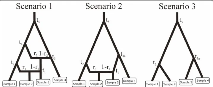
recent to ancient times (see Figure 1). We evaluated the potential of different types of data sets (ten autosomal microsatellite loci, one mtDNA sequence of 1,000 nucleotides, five nuclear autosomal DNA sequences of 1,000 nucleotides each, and all combinations of two and three types of markers) to compare the three competing scenarios and estimate parameters under each scenario.
Prior distributions of demographic parameters were as followed: Uniform[10; 10000] for effective population sizes (similar for all populations), Uniform[1; 100] for t1, Uniform[100; 1000] for t2, Uniform[5000; 50000] for t3, t3a, and t4 (with t4 >t3), Uniform[50000; 500000] for t5, and Uniform[0.1; 0.9] for r1 and r2. For microsa-tellite markers, the ten loci were assumed to follow a generalized stepwise mutation model (GSM [37]) with two parameters: the mean mutation rate (mean μ) and the mean parameter of the geometric distribution of the length in number of repeats of mutation events (mean P) drawn from Uniform[10-4; 10-3] and Uniform[0.1; 0.3] prior distributions, respectively. Each locus has a possible range of 40 contiguous allelic states and was characterized by individual μlocand Plocvalues drawn from Gamma(mean = mean μ and shape = 2) and Gamma(mean = mean P and shape = 2) distributions, respectively [12]. For DNA sequence loci (one mtDNA locus and five nuclear DNA loci), the sequences were assumed to follow the two parameter model of Kimura [34] with a fraction of constant sites (those that cannot mutate) fixed to 10% and the shape parameter of the Gamma distribution of mutations among sites equal to 2. For each sequence locus (1,000 nucleotide per sequence), the mean mutation rate per nucleotide and generation was drawn in a Uniform[10-8; 10-7] and a Uniform[10-9; 10-8] for the mtDNA and nuclear sequences, respectively [53].
The summary statistics for microsatellite loci were the mean number of alleles, expected heterozygosity [38] and allele size variance per population, FST values and genetic distance (δμ)2 between pairs of populations [39,40] and the maximum likelihood estimate of admix-ture proportion [41]. The summary statistics for DNA sequence loci were (i) the number of distinct haplotypes, the number of segregating sites, the mean pairwise dif-ference, the variance of the number of pairwise differ-ences (all statistics computed within each sample), (ii) the number of distinct haplotypes, the number of segre-gating sites (all statistics computed in samples pooled by pair), and (iii) the FST between pairwise samples (com-puted as in [42]) and an adaptation for sequence data of the maximum likelihood estimate of admixture propor-tion of Choisy et al. [41]. Mean values of such statistics were computed over loci grouped by category (microsa-tellites, nuclear DNA sequences and mitochondrial DNA sequence).
For each combination of marker type, we simulated 106 data sets for each of the three competing scenarios. For each competing scenario, we simulated 500 test data sets (i.e. pseudo-observed data sets) drawing demo-graphic and marker parameter values in the same distri-butions as those used to generate the reference table (see legend of Figure 1). For model comparison, we esti-mated the posterior probabilities of the competing sce-narios using a polychotomous logistic regression on the 1% of simulated data sets closest to the observed data set [26]. Posterior probabilities of the three scenarios were used to compute type I and II errors in the choice of each scenario. For instance, let us consider the esti-mation of type I and type II errors when choosing sce-nario 2 as the true scesce-nario. To do so, we simulate 500 data sets according to scenario 1, 2 and 3. Then we count the proportion of times that scenario 2 has not the highest posterior probability among the three com-peting scenarios when it is the true scenario (type I error, estimated from test data sets simulated under sce-nario 2) or the proportion of times that scesce-nario 2 has highest posterior probability when it not the true sce-nario (type II error, estimated from test data sets simu-lated under scenarios 1 and 3).
We then estimated the posterior distributions of para-meters under the most complex scenario (i.e. scenario 1) using a local linear regression on the 1% closest
simulated data sets and applying a logit transformation to parameter values [3,26]. We evaluated the precision of parameter estimation by computing the median of the absolute error divided by the true parameter value of the 500 pseudo-observed data sets simulated under scenario 1 using the median of the posterior distribution as point estimate (RMAE). All computations were pro-cessed using DIYABC V1.0.
Model checking
A combination of a model and parameter posterior dis-tributions is acceptable only if the observed data look similar to replicated data generated under this model-posterior combination (i.e. under the model-posterior predic-tive distribution; [5,20]). To put it another way, the observed data should look plausible under the posterior predictive distribution. This is really a self-consistency check: an observed discrepancy can be due to model misfit (demographic and/or marker models) or chance. Following Gelman et al. ([22] pp 159-163), we imple-mented an option in DIYABC V1.0 to evaluate the dis-crepancy between a model-posterior combination and a target (observed) data set by considering various sets of test quantities. These test quantities are chosen among the set of ABC summary statistics proposed in DIYABC V1.0 (see the notice document available at http://www1. montpellier.inra.fr/CBGP/diyabc for an illustration). For
Figure 1 Evolutionary scenarios to evaluate the interest of mixing microsatellite with mtDNA and/or nuclear DNA sequence data. The three presented scenarios involve different number of divergence and admixture events that occurred at recent to ancient times. Scenario 1 includes six populations, the four that have been sampled (30 diploïd individuals per population) and two unsampled parental populations in the admixture events. The two admixed populations are those represented by samples 2 and 3. Scenario 2 and 3 include five and four populations, respectively. Scenario 2 includes a single admixed population represented by sample 2. Scenario 3 does not include any admixed population. For all scenarios, samples 3 and 4 have been collected 2 and 4 generations earlier than the first two samples, hence their slightly upward locations on the graphs. Time is not at scale. See text of Methods (section“Mixing microsatellite, mtDNA, and/or nuclear DNA sequence data”) for details regarding prior distributions of microsatellite and sequence markers.
each test quantities (t corresponding to the chosen sum-mary statistics), a lack of fit of the observed data with respect to the posterior predictive distribution can be measured by the cumulative distribution function values of each test quantities defined as Prob(tsimulated <t ob-served). Tail-area probability, or p-value, can be easily computed for each test quantities as Prob(tsimulated<t ob-served) and 1.0 - Prob (tsimulated<tobserved) for Prob (t simu-lated<tobserved) ≤ 0.5 and > 0.5, respectively [22]. Such p-values represent the probability that the replicated data (simulated ABC summary statistics) could be more extreme than the observed data (observed ABC sum-mary statistics). Too many observed sumsum-mary statistics on the tails of distributions would cast serious doubts on the adequacy of the model-posterior combination. Because p-values are computed for a number of test sta-tistics, we used the method of Benjamini and Hochberg [43] to control the false discovery rate (see [44] for a comparative study of several methods dealing with false discovery rate control and [23] for an application in the context of an ABC study). An alternative way to com-bine p-values across test statistics has been recently pro-posed [25].
One complication with inferences using ABC is that at least some and sometimes all summary statistics used as tests quantities have already been used during the infer-ence steps (model discrimination and estimation of parameters). There is a risk of over-estimating the qual-ity of the fit by using the same statistics twice. This pro-blem which clearly arises within an ABC framework is actually a general one in statistical inference. As under-lined in many text books in statistics (e.g. [22,45] and see [5]), it is advised against performing model checking using information that have already been used for train-ing (i.e. model fitttrain-ing). Optimally, model checktrain-ing should be based on test quantities that do not corre-spond to the summary statistics that have been used for previous inferential steps; this is naturally possible with DIYABC as the package propose a large choice of sum-mary statistics. The choice of the two sets of statistics remains a difficult issue that still needs to be thoroughly investigated (and that we will not investigate here). In practice, one could advise users to choose the set of sta-tistics for the model discrimination and parameter esti-mation step and the set of statistics for the model checking step before they embark on the first step. Moreover, it seems sensible that both sets include statis-tics describing genetic variation both within and between populations.
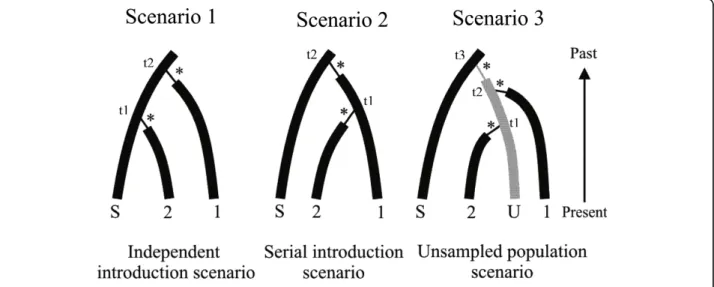
To illustrate this new model checking option of DIYABC V1.0, we have chosen a set of basic scenarios considered when making ABC inferences on the routes of introduction of invasive species [46,47]. We consid-ered three models in which two invasive populations
originate from the same source population. These popu-lations may be related through three different scenarios: the independent introduction scenario, the serial intro-duction scenario and the unsampled population scenario (Figure 2). In the independent or serial introduction sce-narios, all the populations concerned were sampled, but in the unsampled population scenario, the two invasive populations were founded independently from an unde-tected and hence unsampled population, itself intro-duced from the source. It is worth stressing that although previous studies have shown that some inva-sive populations may remain undetected but may play important role in the invasion dynamics of some species [48,49], the unsampled population scenario is often not considered. If only the traditional independent and serial introduction scenarios are compared, a “real” data set obtained under the unsampled population scenario will erroneously fit one of the two competing scenario with often a high posterior probability (see results section and [47]). Here we used a single, randomly chosen, pseudo-observed test data set simulated under the unsampled population scenario to illustrate the interest of the model checking option of DIYABC.
Standard ABC analyses (estimation of model probabil-ities and of parameter posterior distributions) were first performed on the above test data set as described pre-viously (i.e. in the section “Mixing microsatellite, mtDNA and/or nuclear DNA sequence data”). We drew parameter values from the prior distributions described in the legends of Figure 2 and used the summary statis-tics described in Table 1. Model checking computations were then processed by simulating 10,000 data sets under each studied model-posterior combination, with sets of parameter values drawn with replacement among the 10,000 sets of the posterior sample. We computed two groups of test quantities: a first group of summary statistics already used for model discrimination and esti-mation of parameter posteriors and a second group of summary statistics not previously used for inferences. Each observed summary statistics was then ranked and given cumulative distribution function values among the corresponding sample of summary statistics obtained through the above simulation, providing an estimation of p-value for each summary statistics. In addition, a principal component analysis (PCA) was performed in the space of summary statistics. Principal components were computed considering 10,000 data sets simulated with parameter values draw from the prior. Then the target (observed) data set as well as the 1,000 data sets simulated from the posterior distributions of parameters were added to each plane of the PCA. If the model-pos-terior combination fits well the observed data set, one should see on each PCA plane a wide cloud of data sets simulated from the prior, with the observed data set in
the middle of a small cluster of data sets generated from the posterior predictive distribution. All computations and illustrations were processed using DIYABC V1.0.
Results and Discussion
Mixing microsatellite, mtDNA and/or nuclear DNA sequence data
Results dealing with the discrimination among a finite set of competing complex scenarios are summarized in Figure 3. When considering the confidence in scenario choice for each type of markers taken separately, we found that the lowest error rates were obtained for dif-ferent types of markers depending on the type of error and scenario considered. The lowest type I error rates were obtained with the nuclear sequences for scenarios 1 and 2, and microsatellites or mtDNA for scenario 3. The lowest type II error rates were obtained with mtDNA for scenario 1, the nuclear sequences for sce-nario 2 and microsatellites for scesce-nario 3. Some differ-ences in error rates between markers were small, however, and hence not significant using Fisher exact tests (e.g. type II errors for scenario 1 were equal to 0.023 and 0.024 for mtDNA and nuclear sequences, respectively). MtDNA displayed contrasted error rates depending on the scenario considered, with sometimes large error values; for instance a type I error of 0.458
for scenario 1 and a type II of error 0.225 for scenario 2. These large error rates were probably due to the fact that mtDNA data correspond to a single locus and hence to a single gene genealogy subject to substantial stochastic variation [50]. Adding sequence data (mtDNA or nuclear DNA) to microsatellite data globally decreased type I errors (especially for scenario 2 for which type I error was two times lower) and type II errors (especially for scenario 1 for which type I error was two times lower). For all three scenarios, the lowest type I and II error values were obtained when combin-ing the three types of markers.
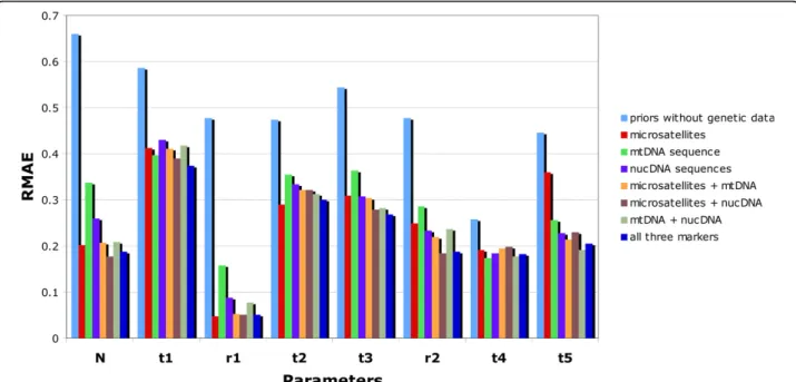
Results dealing with the estimation of parameters under scenario 1 are summarized in Figure 4. Whatever the type and combination of markers, the molecular data provided substantial information for all parameters except the divergence times t1, t2 and t4 for which the level of information remained low. For the latter para-meters the relative median absolute errors (RMAE) were only slightly lower than those computed as base level using only the prior information on parameters (blue bars in Figure 4). This is not surprising since t1 corre-sponds to a very recent time of admixture (< 100 gen-erations) and t2 or t3 correspond to divergence times for which one of the two diverging populations has not been sampled.
Figure 2 Evolutionary scenarios to illustrate model checking. The three presented scenarios are often compared when making ABC inferences on the routes of introduction of invasive species. S is the source population in the native area, and U, the unsampled population in the introduced area that is the source of populations 1 and 2 in scenario 3. The stars indicate the bottleneck events occurring in the first few generations following introductions. We here considered that the dates of first observation were well known so that divergence times could be fixed at 5, 10, 15 and 20 generations for t1, t2, t3 and t4, respectively. The data sets consisted of simulated genotypes at 20 (independent) microsatellite loci obtained from a sample of diploid individuals collected from the invasive and source populations (30 individuals per population). The pseudo-observed test data set that we analyzed to illustrate model checking was simulated under scenario 3 with an effective population size (NS) of 10,000 diploid individuals in all populations except during the bottleneck events corresponding to an effective population size (NFi) of 10 diploid individuals for 5 generations. Prior distributions for ABC analyses (discrimination of scenarios and estimation of posterior distribution of parameters) were as followed: Uniform[1000; 20000] for and logUniform[2; 100] for the demographic parameters NS and NFi, respectively, and same distributions as those given in the text of Methods (section“Mixing microsatellite, mtDNA, and/or nuclear DNA sequence data”) for microsatellite markers.
We found that, depending on the parameter consid-ered, cumulating the information provided by different markers translated into a decrease, an increase or, most frequently, an absence of noticeable variation of the RMAE values compared to that obtained with the most informative genetic marker (Figure 4 and see Additional file 2 for an illustration of the variation of RMAE values expected by chance between different replicates of 500 pseudo-observed data sets). Although each category of markers is different and genealogically independent, the genetic variation at these markers is constrained by the fact that they share the same evolutionary history (i.e. same historical and demographic parameters) so that information provided by each category is not expected to sum up. For all demographic parameters, the lowest RMAE values were obtained, however, when combining the three categories of markers; but in many cases, one or the other category (depending on the considered
parameter), taken alone, provided almost the same precision.
We found that adding sequence data substantially improved the quality of the estimations of some para-meters in comparison to results obtained with microsa-tellites only. This was particularly true for the most ancient divergence time t5 for which RMAE values decreased by 41%, 36% and 47% when adding a single mtDNA sequence, five nuclear sequence and both types of sequences, respectively. Only small decreases of RMAE values were observed for moderately ancient events such as the divergence time t3 and the admixture rate r2. This result underlines the interest of using low mutating and seldom homoplasious sequence data for making inferences on ancient historical events. In agree-ment with this, the two RMAE values for t5 obtained with the mtDNA data sets and the nuclear sequence data sets were lower than that obtained for Table 1 Model checking for introduction scenarios 1, 2 and 3
Probability (tsimulated<tobserved)
Test quantity (t) Observed value Scenario 1 Scenario 2 Scenario 3
Test quantities NAL_S 13.6000 0.7275 0.2871 0.6235
corresponding NAL_1 3.4000 0.7542 0.9865 (*) 0.4252
to thesummary NAL_2 3.6500 0.6455 0.4102 0.4761
statistics used HET_S 0.8429 0.5621 0.2471 0.4488
to discriminate HET_1 0.5151 0.4938 0.9890 (*) 0.4339 among HET_2 0.5725 0.9125 0.9188 0.8221 scenarios and MGW_S 0.8242 0.3593 0.7656 0.5230 compute MGW_1 0.4072 0.3782 0.6713 0.4524 parameter MGW_2 0.4834 0.6117 0.8499 0.7297 posterior FST_S_1 0.2170 0.7882 0.0371 (*) 0.8105 distributions FST_S_2 0.2050 0.6180 0.4606 0.6052 FST_2_3 0.1761 0.0001 (***) 0.9580 (*) 0.6289
Test quantities VAR_S 21.7561 0.7476 0.2538 0.6209
corresponding VAR_1 9.3385 0.4861 0.3561 0.3598
to summary VAR_2 9.5277 0.5232 0.1792 0.3748
statistics NOT LIK_1_S 38.5648 0.7867 0.4503 0.7240
used to LIK_1_2 31.7504 0.0001 (***) 1.0000 (***) 0.7162 discriminate LIK_2_1 32.1075 0.0001 (***) 0.9850 (*) 0.7836 among H2P_S_1 0.7734 0.6563 0.8411 0.6115 scenarios and H2P_S_2 0.7993 0.9231 0.8239 0.8664 compute H2P_1_2 0.6020 0.0315 (*) 0.9975 (**) 0.7193 parameter DAS_S_1 0.1329 0.2298 0.4582 0.2639 posterior DAS_S_2 0.1099 0.0559 0.1681 0.0816 distributions DAS_1_2 0.3402 1.0000 (***) 0.0001 (***) 0.2529
Evolutionary scenarios 1, 2 and 3 are detailed in Figure 3. The single“pseudo-observed” test data set analyzed here was simulated under scenario 3. The probability (tsimulated<tobserved) given for each test quantities (t) was computed from 10,000 data sets simulated from the posterior distributions of parameters
obtained under a given scenario. Corresponding tail-area probabilities, or p-values, of the test quantities (t) can be easily obtained as Prob(tsimulated<tobserved) and
1.0 - Prob (tsimulated<tobserved) for Prob (tsimulated<tobserved)≤ 0.5 and > 0.5, respectively [22]. The test quantities correspond to the summary statistics used to
discriminate among scenarios and compute the posterior distributions of parameters or to other statistics. NAL_i = mean number of alleles in population i, HET_i = mean expected heterozygosity in population i [38], MGW_i = mean ratio of the number of alleles over the range of allele sizes [54], FST_i_j = FSTvalue
between populations i and j [39], VAR_i = mean allelic size variance in population i, LIK_i_j = mean individual assignment likelihoods of population i assigned to population j [22], H2P_i_j = mean expected heterozygosity pooling samples from populations i and j, DAS_i_j = shared allele distance between populations i and j [55]. Populations i and j correspond to populations S, 1 or 2 in Figure 3. *, **, *** = area probability < 0.05, < 0.01 and < 0.001, respectively. Significant tail-area probabilities after applying the false discovery rate correction method of Benjamini and Hochberg [43] are given in bold italic characters.
microsatellite loci only. Due to their mutation modalities (high mutation rates with allele size homoplasy and con-straints [37]), it is not surprising that microsatellite loci performed poorly for ancient evolutionary events [51,52]. On the opposite, microsatellite markers pro-vided substantially better estimation than mtDNA or nuclear sequence for the most recent admixture rate (r1). The RMAE values for the mtDNA sequence and the nuclear sequences were two to three times larger than those obtained with microsatellite only for this parameter. As a result, the addition of mtDNA or nuclear sequences to microsatellite data did not bring any progress in terms of RMAE for r1. This result holds to a lesser extent for the effective population size N. Model checking
When considering altogether the three scenarios in our model discrimination analysis, we found that our (sin-gle) pseudo-observed test data set generated under the unsampled population scenario (scenario 3 in Figure 2) was unambiguously assigned to the correct scenario
with a high posterior probability (p = 0.9967, 95% CI [0.9958, 0.9976]). When only scenarios 1 and 2 were proposed for posterior probability estimation then the same test data set generated under scenario 3 was assigned to the incorrect scenario 2 with a high poster-ior probability (p = 0.9999, 95% CI [0.9998, 1.0000]). Additional ABC treatments achieved on larger sets of pseudo-observed test data sets (n = 1,000) confirmed that if only the traditional independent and serial intro-duction scenarios are considered, a data set obtained under the unsampled population scenario will erro-neously be chosen, with often a high posterior probabil-ity to one of the two competing scenario; scenario 2 is chosen for 55% and 63% of the data sets generated under scenario 3 when simulating test data sets using the same fixed parameter values than the above single test data set and when drawing parameter values in the same distribution than those chosen as priors, respectively.
Focusing on our single pseudo-observed test data set simulated under scenario 3, we evaluated in details the
Figure 3 Confidence in discriminating evolutionary scenarios using microsatellite, mtDNA and/or nuclear DNA sequence data. The three compared scenarios are detailed in Figure 1. Type I error: exclude scenario x when it is actually scenario x. Type II error: choose scenario x when it is not scenario x. Results are based on 500 simulated data sets per scenario with parameter values drawn from the same distributions as the prior distributions given in the legend of Figure 1.
interest of the model checking option of DIYABC V1.0 to assess model misfit. We found that none of the twelve test quantities had low tail probability values when applying the model checking option to the (true) scenario 3 (last column of Table 1). In contrast, one to several test quantities had low tail-area probabilities (sometimes lower than p = 0.001) when applying the model checking option to (incorrect) scenarios 1 or 2, hence casting serious doubts on the adequacy of the tested model-posterior combination. We found some indication of a risk of over-estimating the quality of the fit by using as test quantities the same summary statis-tics already used during the inference steps (model dis-crimination and posterior estimation of parameters); see Table 1. The proportion of test quantities with low tail-area probabilities was indeed larger when using sum-mary statistics not previously used for inference. A close examination of which summary statistics displayed low tail-area probabilities provides some insights on which aspects of the models 1 and 2 are problematic. In the studied case, outlying statistics correspond to an overes-timated genetic differentiation in simulated data sets compared to the observed one between the introduced populations 1 and 2 for scenario 1, whereas it corre-spond to an underestimated genetic differentiation for scenario 2. This pattern is in agreement with the specifi-cities of the “true” scenario 3 (partial genealogical dependency between populations 2 and 3 through the
unsampled population) relatively to scenario 1 (weak genealogical dependency between the independently introduced populations 2 and 3) and scenario 2 (strong genealogical dependency between the serially introduced populations 2 and 3); see Figure 3.
We further inspected the fit/misfit of models by per-forming several principal component analysis on the test quantities obtained with the different model -posterior combinations together with the pseudo-observed test data set simulated under the unsampled population sce-nario (Additional file 3). In agreement with the quantita-tive results summarized in Table 1, the PCA points of the test quantities obtained from the model-posterior combination corresponding to the (true) scenario 3 were nicely grouped and centred on the target point corre-sponding to the pseudo-observed test data set. This con-figuration holds when considering either previously used or unused ABC summary statistics as test quantities. When considering scenarios 1 and 2, we found that the target point of the “pseudo-observed” test data set was positioned at best on the border of the cloud of PCA points of the test quantities corresponding to the sum-mary statistics previously used for ABC analyses. Inter-estingly enough, the target point was clearly outside the cluster when considering unused summary statistics as test quantities.
The model checking analysis of other pseudo-observed test data sets provided results (quantitatively) similar to
Figure 4 Precision in parameter estimation using microsatellite, mtDNA and/or nuclear DNA sequence data under scenario 1. Results are based on 500 pseudo-observed test data sets simulated and estimated under scenario 1 presented in Figure 1, with parameter values drawn from the same distributions as the prior distributions given in the legend of Figure 1. The demographic parameters N, t1, t2, t3, t4, t5, r1 and r2 are detailed in Figure 1. RMAE: relative median absolute errors. The blue columns correspond to the“base-level” RMAE values obtained using only the prior information on parameters (no genetic data).
those presented in the Table 1 and Additional file 3 (results not shown).
Conclusions
The software DIYABC V1.0 offers a user-friendly inter-face allowing non-expert users to perform additional and more accurate inferences using ABC than its pre-vious version. The new implementations allow the treat-ment of haploid in addition to diploid data and allow making inferences from DNA sequence data (without recombination) in addition or separately to microsatel-lite data. The possibility of mixing different types of molecular markers (including autosomal, X or Y-linked loci, and mtDNA loci) should prove useful when consid-ering complex evolutionary scenarios involving both recent and ancient historical events. Finally, DIYABC V1.0 offers non-specialist users a handy way to achieve model checking computation (i.e. the assessment of the “goodness-of-fit” of a model - posterior combination with respect to a target data set), a feature of ABC ana-lysis that has been so far neglected. These new software developments significantly enlarge the tool box available to biologists to make ABC inferences on more complex and hence more realistic demographic processes that have acted on natural populations. The main limitations of the current version of DIYABC are the assumed absence of migration among populations after they have diverged, the impossibility to consider other reproduc-tion systems than standard sexuality as well as evolu-tionary neutrality of markers. Next developments will aim at progressively removing these limitations.
Additional material
Additional file 1: Pre-evaluation of model-prior combinations: two examples. Pre-evaluation of model-prior combinations: example 1. A single test pseudo-observed data set (10 microsatellite loci) was first simulated under a model of a single population (sample size of 30 diploid individuals) with effective size N = 10,000. Microsatellite loci were assumed to follow a generalized stepwise mutation model (GSM [37]) with a mean mutation rate (meanμ) equal to 5 × 10⁻⁴and a mean parameter of the geometric distribution of the length in number of repeats of mutation events (mean P) equal to 0.22. Each locus was given a possible range of 40 contiguous allelic states and was characterized by individualμlocand Plocvalues drawn from Gamma(mean = meanμ and shape = 2) and Gamma(mean = mean P and shape = 2) distributions, respectively [12]. For ABC analysis of the test data set, we used the same population and marker models, and prior distributions of demographic parameters were as followed: Uniform[10; 1000] (figure A) or Uniform [2000; 20000] (figure B) for N, Uniform[10-4; 10-3] and Uniform[0.1; 0.3] for meanμ and mean P, respectively. We choose three summary statistics (s): mean number of alleles, mean expected heterozygosity [38] and mean allele size variance per population. PCA on summary statistics (A and B) and probability (ssimulated<sobserved) for each summary statistics (C) were computed from 10,000 simulations, randomly drawing parameter values from priors. Pre-evaluation of model-prior combinations: example 2. A single pseudo-observed test data set (10 microsatellite loci) was first simulated under a model of two populations (sample size of 30 diploid individuals per population) splitting at time t = 10,000 generations from an ancestral population, without subsequent migration. For all
populations the effective size was N = 1,000. For ABC analysis of the test data set, we used the same population and marker models, and prior distributions of demographic parameters were as followed: Uniform[100; 1000] (figure D) or Uniform[2000; 20000] (figure E) for t, and Uniform[100; 2000] for N. The mutation model and priors for microsatellite markers are the same as in example 1. We choose eight summary statistics (s): mean number of alleles, mean expected heterozygosity [38] and mean allele size variance of each population sample, and FSTvalues and genetic distances (δμ)2between pairs of populations [39,40]. PCA on summary statistics (D and E) and probability (ssimulated<sobserved) for each of the summary statistics (F) were computed from 10,000 simulaxtions, randomly drawing parameter values from priors.
Additional file 2: Evaluation of the variation of RMAE values expected by chance between different replicates of 500 pseudo-observed data sets. relative median absolute errors (RMAE) were computed for 10 replicates of 500 pseudo-observed data sets simulated under scenario 1. The data sets include 20 (independent) microsatellite loci and were generated under scenario 1 presented in Figure 1. Parameter values were drawn from the same distributions than the prior distributions given in the legend of Figure 1. The demographic parameters N, t1, t2, t3, t4, t5, r1 and r2 are detailed in Figure 1. Standard deviation of RMAE values were equal to 0.009, 0.019, 0.004, 0.017, 0.012, 0.013 and 0.014 for N, t1, t2, t3, t4, t5, r1 and r2, respectively. Similar levels of RMAE variation among replicates of 500 pseudo-observed data sets were obtained for other categories of genetic markers (mtDNA and nuclear sequences) and combinations of categories of markers (results not shown).
Additional file 3: Principal component analysis of test quantities when processing model checking for the introduction scenarios 1, 2 and 3. The scenarios 1, 2 and 3 are detailed in Figure 2. The pseudo-observed test data set analyzed here was simulated under scenario 3. PCA were processed on the test quantities corresponding to the summary statistics used to discriminate among scenarios and compute the posterior distributions of parameters (a) or on other statistics (b). The summary statistics used as test quantities are detailed in the legend of Table 1.
Acknowledgements
We thank Gaël Kergoat, Renaud Vitalis and Alexandre Dehne-Garcia for useful discussions. This research was financially supported by the French Agence Nationale de la Recherche grants ANR-09-BLAN-0145-01 to AE, JMC and VR and ANR-07-BDIV-003 (Emerfundis project) to VR.
Author details
1INRA, UMR CBGP (INRA/IRD/Cirad/Montpellier SupAgro), Campus international de Baillarguet, CS 30016, F-34988 Montferrier-sur-Lez cedex, France.2CIRAD, Unité Mixte de Recherche-Biologie et Génétique des Interaction Plante-Parasite, F-34398 Montpellier, France.
Authors’ contributions
JMC and AE carried out the analyses, wrote the paper and jointly developed the software DIYABC v1.0 with VR. All authors read and approved the final manuscript.
Received: 2 April 2010 Accepted: 28 July 2010 Published: 28 July 2010 References
1. Beaumont MA, Rannala B: The Bayesian revolution in genetics. Nat Rev Genet 2004, 5:251-261.
2. Excoffier L, Heckel G: Computer programs for population genetics data analysis: a survival guide. Nat Rev Genet 2006, 7:745-758.
3. Beaumont MA, Zhang WY, Balding DJ: Approximate Bayesian computation in population genetics. Genetics 2002, 162:2025-2035. 4. Bertorelle G, Bonazzo A, Mona S: ABC as a flexible framework to estimate
demography over space and time: some cons, many pros. Mol Ecol 2010. 5. Csilléry K, Blum MGB, Gaggiotti O, François O: Approximate Bayesian
6. Estoup A, Beaumont M, Sennedot F, Moritz C, Cornuet JM: Genetic analysis of complex demographic scenarios: Spatially expanding populations of the cane toad, Bufo marinus. Evolution 2004, 58:2021-2036.
7. Fagundes NJR, Ray N, Beaumont MA, Neuenschwander S, Salzano FM, Bonatto SL, Excoffier L: Statistical evaluation of alternative models of human evolution. Proc Nat Acad Sci USA 2007, 104:17614-17619. 8. Jakobsson M, Hagenblad J, Tavaré S, Säll T, Halldén C, Lind-Halldén C, M N:
A recent unique origin of the allotetraploid species Arabidopsis suecica: evidence from nuclear DNA markers. Mol Biol Evol 2006, 23:1217-1231. 9. Neuenschwander S, Largiader CR, Ray N, Currat M, Vonlanthen P,
Excoffier L: Colonization history of the Swiss Rhine basin by the bullhead (Cottus gobio): inference under a Bayesian spatially explicit framework. Mol Ecol 2008, 17:757-772.
10. Patin E, Laval G, Barreiro LB, Salas A, Semino O, Santachiara-Benerecetti S, et al: Inferring the demographic history of African farmers and Pygmy hunter-gathers using a multilocus resequencing data set. PLoS Genet 2009, 5:e1000448.
11. Rosenblum EB, Hickerson MJ, Moritz C: A multilocus perspective on colonization accompanied by selection and gene flow. Evolution 2007, 61:2971-2985.
12. Verdu P, et al: Origins and Genetic Diversity of Pygmy Hunter-Gatherers from Western Central Africa. Current Biology 2009, 19:1-7.
13. Lombaert E, Guillemaud T, Cornuet J-M, Malausa T, Facon B, Estoup A: Bridgehead effect in the worldwide invasion of the biocontrol harlequin ladybird. PLoS ONE 2010, 5:e9743.
14. Luciania F, Sisson SA, Jiang H, Francis AR, Tanaka MM: The epidemiological fitness cost of drug resistance in Mycobacterium tuberculosis. Proc Natl Acad Sci USA 2009, 106:14711-14715.
15. Ratmann O, Andrieu C, Wiuf C, Richardson S: Model criticism based on likelihood-free inference, with an application to protein network evolution. Proc Natl Acad Sci USA 2009, 106:10576-10581.
16. Beaumont MA, Cornuet JM, Marin JM, Robert C: Adaptive approximated Bayesian computation. Biometrika 2009, 96:983-990.
17. Bortot P, Coles S, Sisson S: Inference for stereological extremes. J Am Statist Assoc 2007, 102:84-92.
18. Leuenberger C, Wegmann D: Bayesian Computation and model selection without likelihoods. Genetics 2009, 184:243-252.
19. Marjoram P, Molitor J, Plagnol V, Tavaré S: Markov chain Monte Carlo without likelihoods. Proc Natl Acad Sci USA 2003, 100:15324-15328. 20. Lopes JS, Beaumont MA: ABC: a useful Bayesian tool for the analysis of
population data. Inf Genet Evol 2009, 10:825-832.
21. Beaumont MA, Nielsen R, Robert C, Hey J, Gaggiotti O, Knowles L, et al: In defence of model-based inference in phylogeography. Mol Ecol 2010, 9:436-446.
22. Gelman A, Carlin JB, Stern HS, et al: Bayesian Data Analysis Chapman and Hall, New York 1995.
23. Ingvarsson PK: Multilocus patterns of nucleotide polymorphism and the demographic history of Populus tremula. Genetics 2008, 180:329-340. 24. Pascual M, Chapuis MP, Mestres F, Balanya J, Huey RB, Gilchrist GW, et al:
Introduction history of Drosophila subobscura in the New World: a microsatellite-based survey using ABC methods. Mol Ecol 2007, 16:3069-3083.
25. Ghirotto S, Mona S, Benazzo A, Paparazzo F, Caramelli D, Barbujani G: Inferring genealogical processes from patterns of bronze-age and modern DNA variation in Sardinia. Mol Biol Evol 2010, 27:875-886. 26. Cornuet JM, Santos F, Beaumont MA, Robert CP, Marin J-M, Balding DJ,
Guillemaud T, Estoup A: Inferring population history with DIYABC: a user-friendly approach to Approximate Bayesian Computation. Bioinformatics 2008, 24:2713-2719.
27. Foll M, Gaggiotti O: A genome-scan method to identify selected loci appropriate for both dominant and codominant markers: a Bayesian perspective. Genetics 2008, 180:977-993.
28. Hickerson MJ, Meyer CP: Testing comparative phylogeographic models of marine vicariance and dispersal using a hierarchical Bayesian approach. BMC Evol Biol 2008, 8:322.
29. Jobin MJ, Moutain JL: REJECTOR: software for population history inference from genetic data via a rejection algorithm. Bioinformatics 2008, 24:2936-2937.
30. Tallmon DA, Koyuk A, Luikart G, Beaumont MA: ONESAMP: a program to estimate effective population size using approximate Bayesian computation. Mol Ecol Res 2008, 8:299-301.
31. Lopes JS, Balding D, Beaumont MA: PopABC: a program to infer historical demographic parameters. Bioinformatics 2009, 25:2747-2749.
32. Wegmann D, Leuenberger C, Neuenschwander S, Excoffier L: ABCtoolbox: aversatile toolkit for approximate Bayesian computations. BMC Bioinformatics 2010, 11:116-122.
33. Jukes TH, Cantor CR: Evolution of protein molecules. Mammalian protein metabolism Academic Press, New YorkMunro HN 1969, 21-123. 34. Kimura M: A simple method for estimating evolutionary rate of base
substitution through comparative studies of nucleotide sequences. J Mol Evol 1980, 16:111-120.
35. Hasegawa M, Kishino H, Yano T: Dating the human-ape splitting by a molecular clock of mitochondrial DNA. J Mol Evol 1985, 22:160-174. 36. Tamura K, Nei M: Estimation of the number of nucleotide substitutions in
the control region of mitochondrial DNA in humans and chimpanzees. Mol Biol Evol 1993, 10:512-526.
37. Estoup A, Jarne P, Cornuet JM: Homoplasy and mutation model at microsatellite loci and their consequences for population genetics analysis. Mol Ecol 2002, 11:1591-1604.
38. Nei M: Molecular Evolutionary Genetics Columbia University Press, New York 1987.
39. Weir BS, Cockerham C: Estimating F-statistics for the analysis of population structure. Evolution 1984, 38:1358-1370.
40. Goldstein DB, Linares AR, Cavalli-Sforza LL, Feldman MW: An evaluation of genetic distances for use with microsatellite loci. Genetics 1995, 139:463-471.
41. Choisy M, Franck P, Cornuet JM: Estimating admixture proportions with microsatellites: comparison of methods based on simulated data. Mol Ecol 2004, 13:955-968.
42. Hudson RR, Slatkin M, Maddison WP: Estimation of levels of gene flow from DNA sequence data. Genetics 1992, 132:583-589.
43. Benjamini Y, Hochberg Y: Controlling the false discovery rate:/a practical and powerful approach to multiple testing. J R Stat Soc B 1995, 57:289-300.
44. Verhoeven KJF, Simonsen KL, McIntyre LM: Implementing false discovery rate control: increasing your power. Oikos 2005, 108:643-647.
45. Dey DK, Rao CR: Bayesian thinking: modelling and computation Handbook of Statistics 25. Elsevier London 2005.
46. Miller N, Estoup A, Toepfer S, Bourguet D, Lapchin L, Derridj S, et al: Multiple transatlantic introductions of the western corn rootworm. Science 2005, 310:992.
47. Guillemaud T, Beaumont MA, Ciosi M, Cornuet JM, Estoup A: Inferring introduction routes of invasive species using approximate Bayesian computation on microsatellite data. Heredity 2010, 104:88-99.
48. Roman J: Diluting the founder effect: cryptic invasions expand a marine invader’s range. Proc R Soc B 2006, 273:2453-2459.
49. Saltonstall K: Cryptic invasion by a non-native genotype of the common reed, Phragmites australis, into North America. Proc Natl Acad Sci USA 2002, 99:2445-2449.
50. Degnan JH, Rosenberg NA: Gene tree discordance, phylogenetic inference and the multispecies coalescent. Tr Ecol Evol 2009, 24:332-340. 51. Takezaki N, Nei M: Genetic distances and reconstruction of phylogenetic
trees from microsatellite DNA. Genetics 1996, 144:389-399. 52. Pollock DD, Bergman A, Feldman MW, Goldstein DB: Microsatellite
behavior with range constraints: parameter estimation and improved distances for use in phylogenetic reconstruction. Theoret Pop Biol 1998, 53:256-271.
53. Haag-Liautard C, Coffey N, Houle D, Lynch M, Charlesworth B, Keightley PD: Direct estimation of the mitochondrial DNA mutation rate in Drosophila melanogaster. PLoS Biol 2008, 6:e204.
54. Excoffier L, Estoup A, Cornuet JM: Bayesian analysis of an admixture model with mutations and arbitrarily linked markers. Genetics 2005, 169:1727-1738.
55. Jin L, Chakraborty R: Estimation of Genetic Distance and Coefficient of Gene diversity from Single-Probe Multilocus DNA Fingerprinting Data. Mol Biol Evol 1993, 11:120-127.
doi:10.1186/1471-2105-11-401
Cite this article as: Cornuet et al.: Inference on population history and model checking using DNA sequence and microsatellite data with the software DIYABC (v1.0). BMC Bioinformatics 2010 11:401.