HAL Id: hal-02406957
https://hal.archives-ouvertes.fr/hal-02406957
Submitted on 17 Jun 2020HAL is a multi-disciplinary open access
archive for the deposit and dissemination of sci-entific research documents, whether they are pub-lished or not. The documents may come from teaching and research institutions in France or abroad, or from public or private research centers.
L’archive ouverte pluridisciplinaire HAL, est destinée au dépôt et à la diffusion de documents scientifiques de niveau recherche, publiés ou non, émanant des établissements d’enseignement et de recherche français ou étrangers, des laboratoires publics ou privés.
to deep basin in spring to summer transition in the
Arctic Ocean
Barbara Oleszczuk, Emma Michaud, Nathalie Morata, Paul Renaud, Monika
Kędra
To cite this version:
Barbara Oleszczuk, Emma Michaud, Nathalie Morata, Paul Renaud, Monika Kędra. Ben-thic macrofaunal bioturbation activities from shelf to deep basin in spring to summer transi-tion in the Arctic Ocean. Marine Environmental Research, Elsevier, 2019, 150, pp.104746. �10.1016/j.marenvres.2019.06.008�. �hal-02406957�
Please note that this is an author-produced PDF of an article accepted for publication following peer review. The definitive publisher-authenticated version is available on the publisher Web site.
Marine Environmental Research
September 2019, Volume 150, Pages 104746 (16p.)
https://doi.org/10.1016/j.marenvres.2019.06.008 https://archimer.ifremer.fr/doc/00502/61329/
Archimer
https://archimer.ifremer.fr
Benthic macrofaunal bioturbation activities from shelf to
deep basin in spring to summer transition in the Arctic
Ocean
Oleszczuk Barbara 1, *, Michaud Emma 2, Morata Nathalie 2, 3, Renaud Paul E. 3, 4, Kędra Monika 1
1 Institute of Oceanology, Polish Academy of Science (IOPAN), Powstańców Warszawy 55, 81-712, Sopot, Poland
2 Laboratoire des Sciences de L'environnement Marin Sciences (LEMAR), UMR 6539 (CNRS/UBO/ IRD/Ifremer), Institut Universitaire Européen de la Mer, rue Dumont d’Urville, 29280, Plouzané, France 3 Akvaplan-niva, Fram Centre for Climate and the Environment, Tromsø, Norway
4 The University Centre in Svalbard, Longyearbyen, Norway
* Corresponding author : Barbara Oleszczuk, email address : [email protected]
Abstract :
The aim of this study was to assess bioturbation rates in relation to macrozoobenthos and environmental variables in the Svalbard fjords, Barents Sea and Nansen Basin during spring to summer transition. The results showed differences in benthic community structure across sampled area in relation to sediment type and phytopigment content. Fjords, Barents Sea and the shallow parts of Nansen Basin (<400 m) were characterized by high functional groups diversity, and by biodiffusive and non-local rates ranging from 0.05 to 1.75 cm−2 y−1 and from 0.2 to 3.2 y−1, respectively. The deeper parts of Nansen Basin, dominated by conveyors species, showed only non-local transport rates (0.1–1 y−1). Both coefficients intensity varied with benthic biomass. Non-local transport increased with species richness and density and at stations with mud enriched by fresh phytopigments, whereas biodiffusion varied with sediment type and organic matter quantity. This study quantified for the first time the two modes of sediment mixing in the Arctic, each of which being driven by different environmental and biological situations.
Highlights
► This is the first complex report on bioturbation in spring to summer transition conducted over a large depth gradient in the Arctic Ocean. ► Benthic community structure and related biodiffusion and non-local transport varied in Svalbard fjords, Barents Sea and Nansen Basin. ► Changes in environmental conditions, and related changes in quality and quantity of available organic matter, had impact on benthic communities and bioturbation. ► Large inputs of fresh OM to the seabed can trigger bioturbation activities.
Keywords : non-local transport, biodiffusive transport, macrozoobenthos, spring season, sea ice cover, Arctic
M
AN
US
CR
IP
T
AC
CE
PT
ED
2 Abstract 26The aim of this study was to assess bioturbation rates in relation to macrozoobenthos and 27
environmental variables in the Svalbard fjords, Barents Sea and Nansen Basin during spring 28
to summer transition. The results showed differences in benthic community structure across 29
sampled area in relation to sediment type and phytopigment content. Fjords, Barents Sea and 30
the shallow parts of Nansen Basin (<400 m) were characterized by high functional groups 31
diversity, and by biodiffusive and non-local rates ranging from 0.05 to 1.75 cm-2 y-1 and from 32
0.2 to 3.2 y-1, respectively. The deeper parts of Nansen Basin, dominated by conveyors 33
species, showed only non-local transport rates (0.1 to 1 y-1). Both coefficients intensity varied 34
with benthic biomass. Non-local transport increased with species richness and density and at 35
stations with mud enriched by fresh phytopigments, whereas biodiffusion varied with 36
sediment type and organic matter quantity. This study quantified for the first time the two 37
modes of sediment mixing in the Arctic, each of which being driven by different 38
environmental and biological situations. 39
40
Key words: non-local transport; biodiffusive transport; macrozoobenthos; spring season; sea 41
ice cover; Arctic Ocean
42 43
1. Introduction
44 45
The structure and functioning of benthic communities depend on the quality and quantity 46
of organic matter (OM) export fluxes to the sea floor and this dependence increases with 47
increasing depth. Shallow Arctic shelves benthos is often fueled by high OM fluxes to the sea 48
floor due to tight pelagic-benthic coupling (e.g. Grebmeier et al., 2006; Tamelander et al., 49
2008), while deep-sea communities become food-limited due to low amount of OM reaching 50
M
AN
US
CR
IP
T
AC
CE
PT
ED
3sea floor (Maiti et al., 2010). The seasons strongly shape the OM fluxes to the sea floor in the 51
Arctic marine ecosystems. Phytoplankton and ice algae are two principal sources of primary 52
production (PP) in the Arctic Ocean with ice algae being the first food source available after 53
polar night (Søreide et al., 2006, 2008; Leu et al., 2010). Although phytoplankton is 54
quantitatively dominant, ice algal blooms tend to occur earlier in the seasonally ice-covered 55
Arctic seas and may contribute up to 50–60% of total PP (Gosselin et al., 1997; McMinn et 56
al., 2010; Fernandez-Mendez et al., 2015; Van Leeuwe et al., 2018). During the spring, PP is 57
typically greater than zooplankton consumption and thus highest vertical carbon fluxes are 58
recorded (Andreassen and Wassmann, 1998; Tamelander et al., 2006). Later in the season, the 59
zooplankton grazing reduces the OM flux but also adds to it by producing fecal pellets, which 60
helps phytoplankton sink rapidly to the sea bottom (Olli et al., 2002). In fjords and on the 61
shelf, benthic communities can also be fueled by terrestrial OM carried by rivers and/or 62
glaciers, mainly during summer (Bourgeois et al., 2016). Benthic organisms act as temporal 63
couplers in the seasonal systems, since they can consume variable carbon sources over the 64
different seasons (McMeans et al., 2015), therefore benthic communities reflect rather long 65
term (months to years) water column production, while the benthic activities reflect short term 66
(days to weeks) environmental conditions (Morata and Renaud, 2008). 67
Bioturbation occurs when an organism moves through the sediment, constructs and 68
maintains burrows, and ingests and defecates. This process results in mixing of particles and 69
solutes within the substratum (Kristensen et al., 2012), and alters sediment structure (e.g., 70
grain size distribution; Montserrat et al., 2009), and production, mineralization and 71
redistribution of OM (Kure and Forbes, 1997). Life habit, motility, and manner of feeding of 72
infaunal species induce either random particle movement over a short distance (biodiffusion 73
(Db) hereafter) (Gérino et al., 2007; Meysman et al., 2003) or biologically induced 74
discontinuous particle transfer between the sediment surface and deeper sediment layers, for 75
M
AN
US
CR
IP
T
AC
CE
PT
ED
4example via burrowing or feeding behavior (non-local transport (r) hereafter) (Boudreau, 76
1986; Meysman et al., 2003; Duport et al., 2007; Gogina et al., 2017). According to the mode 77
of particle mixing, benthic organisms can be classified into five functional groups of sediment 78
reworking which may include biodiffusion and/or non-local transport: biodiffusors, gallery-79
diffusors, upward- and downward-conveyors, and regenerators (François et al., 1997). The 80
presence and intensity of these bioturbation modes are therefore mediated by fauna 81
characteristics like biomass, density, burrowing depth or feeding behavior (François et al., 82
1999; Gérino et al., 1998; Sandnes et al., 2000; Gilbert et al., 2007; Michaud et al., 2005,
83
2006; Duport et al., 2007; Aschenbroich et al., 2017). In turn, species composition, nature and
84
intensity of their effects on sediment mixing depends on temperature (Ouelette et al., 2004; 85
Duport et al., 2007; Maire et al., 2007), food inputs (Nogaro et al., 2008) and sediment 86
characteristics (Needham et al., 2011). Changes in species composition and activities, and 87
therefore in bioturbation mode and/or intensity, are expected to influence biochemical 88
processes near the sediment-water interface, including carbon cycling. Bioturbation rate can 89
therefore be influenced by seasonal changes in PP in the above water column and deposited 90
OM in the seafloor (food bank; Morata et al., 2015). 91
Only a few studies of bioturbation exist in the Arctic Ocean. Teal et al. (2008) created 92
the database with global bioturbation intensity coefficient (Db) and layer depth (L), where 93
they showed that the Arctic, Central Pacific and most tropical regions are missing bioturbation 94
data. In polar regions, it has been shown that sediment mixing rates were higher through 95
biological transports in the shallow sediments directly impacted by the OM input along the 96
marginal ice covered area of the Barents Sea (Maiti et al., 2010) and in the Svalbard fjords 97
(Konovalov et al., 2010). On the contrary, the deep sediments of the Arctic Ocean were 98
marked by lower sediment mixing rates in relation to a lower benthic biomass correlated with 99
lower OM inputs (Clough et al., 1997). Soltwedel et al. (2019), however, did not confirm a 100
M
AN
US
CR
IP
T
AC
CE
PT
ED
5higher bioturbation activity in the high productive Marginal Ice Zone (MIZ) in Fram Strait 101
compared to the less productive ice zone. Seasonal aspects of bioturbation in the Arctic were 102
preliminarily studied by Morata et al. (2015), whose experiments showed that the bioturbation 103
activity was positively correlated with fresh food input during the polar night. McClintic et al. 104
(2008) found no seasonal variation in bioturbation intensity during June and October in West 105
Antarctic continental shelf which suggests that deposit feeders are able to access food 106
particles accumulated during high PP periods. Still, our knowledge on benthic communities 107
responsible for bioturbation processes and their relation to OM inputs in the Arctic Ocean and 108
adjacent shelves remains limited, particularly during the spring bloom. 109
The main aim of this study was to understand the impacts of differences in 110
environmental conditions on benthic communities and their bioturbation function during the 111
spring to summer transition. We focused on the Svalbard area where fjords, shelf and deep 112
Nansen Basin differ considerably in terms of physical forcing affecting the quality and 113
quantity of the OM inputs to the seafloor. Sediment reworking rates were quantified in 114
relation to taxonomic and functional composition of the benthic macrofaunal communities, 115
and in relation to the environmental variables. This work is the first study on bioturbation 116
processes conducted in the Arctic Ocean during spring to summer transition time over a large 117
depth gradient. It will contribute to our understanding of response of macrofauna and their 118
activity to the quality and quantity of OM in the Arctic seabed. 119
120
2. Material and methods
121 122
2.1. Study area
123 124
M
AN
US
CR
IP
T
AC
CE
PT
ED
6Sampling was conducted in the Svalbard Archipelago, the Barents Sea and deep Nansen 125
Basin north of Svalbard (Fig. 1, Table 1). This area is highly influenced by cold Arctic Water 126
coming from the north and warm Atlantic Waters coming from the south, and the relative 127
influence of those two water masses varies largely in the study area. 128
129
130
Fig. 1. Geographical location of the study region (A) and (B) sampling locations during two 131
cruises (AX – ARCEx, PS – TRANSSIZ) with two major currents surrounding Svalbard: 132
M
AN
US
CR
IP
T
AC
CE
PT
ED
7WSC - West Spitsbergen Current, warm Atlantic waters (black) and the ESC – East 133
Spitsbergen Current, cold Arctic waters (gray) (after Svendsen et al., 2002). 134
M
AN
US
CR
IP
T
AC
CE
PT
ED
8Table 1. Main characteristics of the sampling stations.
135
Station Date Cruise name No of
cores Area Latitude (°N) Longitude (°E) Main current Depth [m] Bottom Water Salinity Bottom Water Temperature (°C) AX/1 19.05.2016 ARCEx 5 Van Mijenfjorden 77.83° 16.47° ESC 59 34.5 -0.8
AX/2 20.05.2016 ARCEx 5 Hornsund 77.02° 16.45° ESC 121 34.5 -0.8
AX/3 21.05.2016 ARCEx 5 Storfjorden 77.94° 20.22° ESC 96 34.5 -0.8
ST/8 15.07.2016 SteP 4 Storfjorden 77.98° 20.28° ESC 99 34.1 4.5
AX/4 24.05.2016 ARCEx 5 Erik Eriksen Strait 79.21° 26.00° ESC 217 34.7 0.5
AX/6 25.05.2016 ARCEx 5 Southern Barents Sea 76.60° 30.01° ESC 278 35.0 2.5
PS/20 30.05.2015 TRANSSIZ 3 Northern Barents Sea 81.04° 19.32° WSC 170 34.9 0.9
PS/32 06.06.2015 TRANSSIZ 4 Northern Barents Sea 81.16° 20.01° WSC 312 34.9 2.1
PS/19 29.05.2015 TRANSSIZ 5 Northern Barents Sea 81.23° 18.51° WSC 471 35.1 1.4
PS/27 01.06.2015 TRANSSIZ 5 Northern Barents Sea 81.31° 17.15° WSC 842 34.9 0.2
PS/31 04.06.2015 TRANSSIZ 5 Nansen Basin 81.47° 18.17° WSC 1656 34.9 2.5 136
137 138 139
M
AN
US
CR
IP
T
AC
CE
PT
ED
9Van Mijenfjorden and Hornsund are located on the west coast of Spitsbergen, 140
Svalbard. Van Mijenfjorden is a small fjord, nearly closed by an island at its mouth. It is 141
separated into two basins: the outer (115 m depth) and inner (74 m depth), and by 45 m deep 142
sill that restricts exchange of water between the fjord and the coastal waters (Skarđhamar and 143
Svendsen, 2010). Hornsund is a large open glacial fjord with eight major tidal glaciers located 144
in the central and inner parts and large terrestrial inflow (Błaszczyk et al., 2013; Drewnik et 145
al., 2016). The average depth is 90 m with a maximum of 260 m (Kędra et al., 2013). Strong 146
gradients in sedimentation, PP and benthic fauna occur along the increasing distance to the 147
glaciers (Włodarska-Kowalczuk et al., 2013). These high latitude fjords are productive 148
systems, where PP starts in early spring and continue to late autumn (Fetzer et al., 2002). The 149
annual PP reaches up to 216 g C m-2 y-1 in Hornsund (Smoła et al., 2017). The Barents Sea is 150
a shelf sea with water depths ranging from 35 m in the Svalbard Bank to up to 400 m or more 151
in deep depressions and proximal canyon boundaries (Cochrane et al., 2012). The southern 152
part of the Barents Sea is relatively warm and ice free while its northern parts are seasonally 153
ice covered, with maximum ice coverage from March to April and minimum ice coverage 154
generally occurring in September (Vinje, 2009; Ozhigin et al., 2011; Jørgensen et al., 2015). It 155
is one of the most productive areas in the Arctic Ocean with average PP about 100 g C m-2 y -1 156
and maximum PP reaching over 300 g C m-2 y -1 on shallow banks (Sakshaug, 2004). 157
Storfjorden is located east of Spitsbergen and has a maximum depth of 190 m (Skogseth et al., 158
2005). A polynya appears regularly in Storfjorden. It is a very productive area of the Barents 159
Sea, and its productivity is correlated with the duration of the seasonal sea cover 160
(Winkelmann and Knies, 2005). In Storfjorden the production of marine organic carbon may 161
exceed 300 mg C cm-2 kyr-1, while the production of total organic carbon (TOC) may exceed 162
500 mg C cm-2 kyr-1 (Pathirana et al., 2013; Rasmussen and Thomsen, 2014). Nansen Basin, 163
M
AN
US
CR
IP
T
AC
CE
PT
ED
10with a maximum depth of 4000 m, is part of the Eurasian basin of the Arctic Ocean. In 164
general, annual gross PP is within the range of 5–30 g C m-2 (Codispoti et al., 2013). 165
166
2.2. Sampling
167 168
Benthic sampling was conducted during spring cruises of R/V Polarstern PS92 – 169
TRANSSIZ in May and June 2015, and R/V Helmer Hanssen – ARCEx in May 2016 (Table 170
1). Samples were collected at 10 stations located along the depth gradient, from Svalbard 171
fjord (depth: 59 – 121 m), through the Barents shelf and slope (from 170 to 842 m) to the 172
deep Nansen Basin (max. depth: 1656 m) (Fig. 1). Almost all stations north of Svalbard (P32, 173
PS/19, PS/27 and PS/31) were sea ice covered during sampling, except PS/20 station. One 174
station in Storfjorden (AX/3) was revisited in July 2016 during the cruise of R/V L’Atalante – 175
STeP 2016 (ST/8). 176
At each station the bottom water temperature and salinity were determined by the 177
shipboard Conductivity Temperature Density (CTD) rosette. Bottom-water samples were 178
collected using Niskin bottles attached to a CTD and were filtered on pre-combusted 179
Whatman GF/F glass microfiber filters in triplicate and frozen at -20 °C for later analyses of 180
bottom water organic carbon (BW Corg), total nitrogen (BW Ntot), δ13C (BW δ13C), δ15N (BW 181
δ15N), and C/N ratio (BW C/N). 182
Sediment samples were collected with a box corer of 0.25 m2 sampling area. The 183
overlying water from box corer was gently removed from sediment surface and push-cores 184
samples (12 cm Ø and 20 cm deep, 113.0940 cm2 surface layer) were collected. The top 2 cm 185
sediment of the core was sampled for biogeochemical variables (grain size, chlorophyll a (Chl 186
a) and phaeopigments (Phaeo), organic matter (SOM), organic carbon (Sed Corg) and total 187
M
AN
US
CR
IP
T
AC
CE
PT
ED
11nitrogen (Sed Ntot)). Samples were frozen in -20 °C and transported to the laboratory for 188
analysis. 189
Additional sediment cores were taken from the box corer for bioturbation experiments 190
following procedures described by Morata et al. (2015). Sediment cores (3 to 5 per station, 191
Table 1) were kept in dark cold room on board (i.e., temperature at 2 °C, the average between 192
-0.8°C and 4.5°C being the range of temperatures observed in the bottom waters, Table 1). 193
Fluorescent luminophores (5 g; 90–120 µm diameter) were homogeneously added to 194
the overlying water and gradually spread on the sediment surface of each core without 195
disturbing the resident infauna. Cores were then filled with bottom water and aerated by 196
bubbling to keep the overlying water saturated with oxygen. Overlying water was renewed 197
every four days. Sediment cores were incubated in those conditions for 10 days which is the 198
minimum time to enable the characterization of the different transport modes. Incubation time 199
that exceeds 15 days increases the probability of complete homogenization of the sedimentary 200
column, and may thus prevent the differentiation of transport modes (François et al., 1997). 201
This choice of 10 days for duration of experiment was a compromise between the response 202
that we were expecting from the benthic communities and the available time on board to 203
process the experiments. 204
After this time of incubation in stable conditions the surface water was carefully 205
removed and cores were sliced horizontally in 0.5 cm layers from 0 to 2 cm depth, and in 1 206
cm layers between 2 and 10 cm depth. In total, 12 samples were taken, and each sediment 207
layer was homogenized. A subsample of each sediment layer was directly frozen (-20 °C) and 208
used for bioturbation analyses. The remaining sediment of each core samples were sieved 209
onboard through 0.5 mm sieve for benthic community structure analysis, and fixed with 10 % 210
buffered formaldehyde. 211
M
AN
US
CR
IP
T
AC
CE
PT
ED
122.3. Biogeochemical environmental analyses
213 214
Sediments for grain size analysis were freeze-dried at -70 °C, homogenized and dry 215
sieved into coarse-grained fractions (>0.250 mm) and fine-grained (<0.250 mm). For the fine 216
fraction, analyses were performed using a Malvern Mastersizer 2000 laser particle analyzer 217
and presented as volume percent. Mean grain size parameters were calculated using the 218
geometric method of moments in the program GRADISTAT 8.0 (Blott and Pye, 2001). 219
Pigment concentrations were analyzed fluorometrically following methods described 220
in Holm-Hansen et al. (1965) to determine Chl a and Phaeo concentrations. About 1 g of dried 221
sediment was extracted with 10 ml of 90 % acetone at 4 °C in the dark. After 24 h, sediment 222
was then centrifuged (3000 rpm for 2 min), and analysed using a Turner Designs AU-10 223
fluorometer before and after acidification with 100 µl 0.3 M HCl. 224
For sediment and bottom water biogeochemical parameters analyses, sediments and 225
filters were dried, homogenized and weighed into silver capsules. For sediment and bottom 226
water δ13C and δ15N, Corg and Ntot analyses, samples were acidified with 2 M HCl to remove 227
inorganic carbon and dried at 60 °C for 24 h. The analyses were performed on an Elemental 228
Analyzer Flash EA 1112 Series combined with an Isotopic Ratio Mass Spectrometer IRMS 229
Delta V Advantage (Thermo Electron Corp., Germany). SOM content was measured as loss 230
on ignition at 450°C for 4 h (Zaborska et al., 2006). Sed Corg content was measured following 231
the method of Kennedy et al. (2005). About 10 mg of dried sediment was acidified with 50 µl 232
of 1 N HCl three times. Analyses were run on a Thermo Quest Flash EA 1112 CHN analyzer. 233
234
2.4. Benthic community analysis
235 236
M
AN
US
CR
IP
T
AC
CE
PT
ED
13In the laboratory, macrofaunal organisms were picked from sediments under a binocular 237
microscope and identified to the lowest possible taxonomic level. Each taxon was counted, 238
weighed (g wet weight) and transferred to 70 % ethanol. Mobility and feeding (WoRMS 239
Editorial Board, 2019), and burrowing behavior (for references see Table 4) were attributed to 240
each taxon. Benthic fauna was classified into five bioturbation functional groups based on the 241
type of the sediment mixing: biodiffusors, gallery-diffusors, upward- or downward-conveyors, 242
and regenerators. Biodiffusors move particles in a random manner in short distances (Gérino, 243
1992). Gallery-diffusors transport material from the surface sediment layer to deeper by 244
constructing tubes or tunnels system (François et al., 2002). Upward-conveyors transport 245
material from depth to the sediment surface and downward-conveyors transport sediment non-246
locally to deeper layers (Fisher et al., 1980; Knaust and Bromley, 2012). Regenerators create a 247
biodiffusion-like process, with large amounts of sediment transported out of the reworked 248
zone with a strong input to the overlying water column, as well as passive downward 249
transport of surface sediment to the bottom of the burrow after burrow abandonment (Gardner 250
et al., 1987; Knaust and Bromley, 2012). Organism density and biomass were evaluated per 251
taxon, trophic and bioturbation functional group, and in total for each sediment core, and 252
subsequently converted per 1 m-2 (area) in order to provide relevant surface values. The 253
biomass to density (B/D) ratio was calculated per core as a proxy of the mean organism size. 254
255
2.5. Bioturbation analyses
256 257
After the sediment cores were sliced, part of the sediment from each sediment layer 258
was freeze-dried at -70 °C, and homogenized with a mortar and pestle. Three replicates of 0.2 259
g sediment from each layer were taken and placed on a black box (9.5 cm x 7 cm) under a 260
constant UV light source (350 ± 370 nm, Tube UV BLB G5T5 6 W). Images were taken with 261
M
AN
US
CR
IP
T
AC
CE
PT
ED
14a digital camera (Nikon digital captor 2.342.016 pixels) with 28 µm per pixel resolution from 262
a constant 12 cm from the sediment sample to assure identical acquisition conditions for all 263
images (aperture time 1 s; diaphragm aperture f/13, ISO 200). Images were saved in
red-264
green-blue (RGB) colour in jpeg format. The images were analysed using an image 265
processing toolbox (@mathworks) in order to differentiate luminophores from the background 266
sediment by using an appropriate set of RGB threshold levels (Michaud, 2006). Finally, the 267
particle size appropriate for each luminophore was selected (6 pixels × 6 pixels for the 268
smallest luminophores), and the pictures were corrected (cleaned) by removing the particle 269
sizes smaller and larger than the actual size of the specific luminophore (90–120 µm). The 270
sum of areas (in pixels) of the remaining objects and the number of objects (i.e., 271
luminophores) were calculated for each picture and averaged between the three pictures from 272
each sediment layer. Finally, with these abundances for all sediment depths for each core, the 273
results were computed as the percentage of detected pixels per depth according to the total 274
number of pixels detected per core thus representing the luminophores distribution over depth 275
for each sediment core. 276
The reaction diffusion type model used in this paper to describe luminophore 277
redistribution following macrofaunal reworking is based on the general diagenetic equation 278
(Berner,1980): 279
= + (1)
280
where Q is the quantity of the tracer (e.g., luminophores), t is the time, z is the depth, Db is 281
the apparent biodiffusion coefficient, and r(Q) is the non-continuous displacement of tracer. 282
The term r(Q) is defined as follows: 283 , = , ∈ !; #$ %! & − , ∈ 0; ! 0 > # (2a-c) 284
M
AN
US
CR
IP
T
AC
CE
PT
ED
15where ! and # define the upper and lower limits of the tracer redistribution, x and z are 285
depth variables and r is the biotransport coefficient that is the percentage of tracer that left the 286
[0; !] deposit and was redistributed in the [ !; #] layer. The redistribution of tracer between 287
! and # and the disappearance of tracer from the 0- ! layer are, respectively, described by 288
Eqs. (2a) and (2b). Eq. (2c) indicates that no tracer movement occurs below #. 289
This displacement term was originally exemplified in a model describing gallery-290
diffusion of macrofaunal reworking (François et al., 2002). This biological reworking process 291
describes the diffusive-like mixing of particles in the region of intense burrowing activity and 292
the rapid transport of organic and inorganic material from the upper sediment layers to the 293
lower regions of reworking (i.e. ‘biotransport’ or “non-local transport”). 294
According to the experimental conditions, the following initial conditions were used: 295
, * = + & ∈ !; #
* ,-., (3)
296
where [ !; #] is the tracer deposit layer. Finally, a zero-flux Neuman boundary condition was 297
considered: 298
0, = lim →∞ , = 0 (4)
299
The application of this bioturbation model to tracer redistributions, initially started by 300
François et al. (1997, 2001) and later revised by Duport al., (2007), allowed the quantification 301
of two particle mixing coefficients: an apparent biodiffusion coefficient Db and a biotransport 302
coefficient r. The biodiffusion coefficient Db takes into account the diffusion-like transport 303
due to the activity of the organisms. We assume that the actual concentration dependent 304
diffusion of tracers is negligible. The biotransport coefficient (r) represents a non-local mixing 305
pattern associated with a biologically induced transfer of particles from one place to another 306
in a discontinuous pattern (i.e. a non-continuous transport; Boudreau, 1986; Meysman et al., 307
2003). Estimates of the parameters Db and r were finally obtained by minimizing a weighted 308
sum of squared differences between observed and calculated tracer concentrations (François 309
M
AN
US
CR
IP
T
AC
CE
PT
ED
16et al., 1999, 2002). For each core, many adjustments between the observed and modelled 310
profiles are necessary in order to find the minimum weighted sum of squared differences. 311
This model was used with MatLab (@mathworks), thus it gives qualitative data (i.e., 312
kind of sediment mixing) and quantitative data (intensity of the sediment mixing) on the 313
sediment mixing function for the entire benthic community at the sediment-water interface. 314
315
2.6. Statistical analysis
316 317
Bray-Curtis similarity matrix, based on square-root transformed data was used for the 318
multivariate analysis of the macrobenthic community. Principal coordinate analysis (PCO) 319
was conducted to explore multivariate variability among different sampling stations based on 320
the (B/D) ratio community composition data matrix. Pearson rank correlation (>0.5) vectors 321
of species B/D with axes were overlaid on the PCO plots to visualize the relationships 322
between ordination axes and the directions and degrees of variability in the biological 323
variables. Differences in species composition in samples among the groups of stations were 324
explored using non-parametric multivariate methods applied to Bray-Curtis dissimilarity 325
matrix calculated from biomass/density ratio (B/D) (one-way PERMANOVA). Whenever the 326
significant effect of factor was detected by the main PERMANOVA test, pair-wise tests for 327
differences between levels of each significant factor was performed. SIMPER procedure 328
(similarity percentage species contribution) was used to discriminate species responsible for 329
the differences between sites. In all models, a forward-selection procedure was used to 330
determine the best combination of predictor variables for explaining the variations in 331
macrofauna assemblages. The selection criteria chosen for the best-fitting relationship were 332
based on R2 values (Anderson et al. 2008). A distance-based linear model (DistLM) was used 333
to analyse and model the relationships between the macrofaunal community structure and the 334
M
AN
US
CR
IP
T
AC
CE
PT
ED
17environmental factors. A distance-based redundancy analysis (dbRDA) was used to visualize 335
the variability along the two axes that best discriminated groups of samples defined by a priori 336
assigned groups. Superimposed vectors corresponded to Pearson's correlations (>0.5) of 337
environmental factors with the dbRDA axes. Calculations of the pseudo-F and p values were 338
based on 999 permutations of the residuals under a reduced model. The significance level for 339
all the statistical tests was p = 0.05. 340
The normality of environmental factors and biological factors (non-local and biodiffusion 341
coefficients, benthic density and biomass) was verified with use of Shapiro-Wilk test 342
(p<0.05). Since data did not have a normal distribution, Spearman correlations were 343
calculated to estimate the relationships between faunal community characteristics (Table 8) 344
and environment (Appendix 1). Differences in benthic density, biomass, non-local and 345
biodiffusion coefficient were evaluated with the use of the nonparametric Kruskal-Wallis test, 346
and the Dunn’s post-hoc multiple comparison test was applied to identify the differences 347
among stations groups. Station ST/8, sampled in July, was excluded from those analyses due 348
to lack of environmental information and because it was sampled during a different season 349
than the other stations. Additionally, a non-parametric pairwise Mann-Whitney U-test was 350
performed to compare differences between the spring and summer season in Storfjorden 351
(AX/3 vs ST/8). All analyses were performed using the PRIMER package v. 7 Clarke and 352
Gorley, 2006; Anderson et al., 2008) and the Statsoft software STATISTICA v. 9. 353 354 3. Results 355 356 3.1. Environmental patterns 357 358
M
AN
US
CR
IP
T
AC
CE
PT
ED
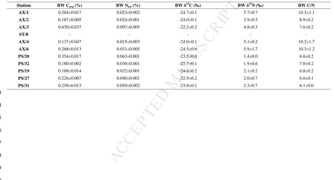
18Bottom water salinity ranged from 34.5 to 35.1 and bottom water temperature ranged 359
from -0.8 °C to 2.5 °C during our sampling. The lowest BW Corg concentrations were 360
measured in Erik Eriksen Strait (AX/4; 0.1 ± 0.1 %) and the highest in Storfjorden (AX/3; 0.6 361
± 0.0 %). The BW δ13C values ranged from -27.7‰ on the slope north of Svalbard (PS/32) to 362
-22.2 ‰ in Storfjorden. The lowest BW C/N ratio values were found at the deepest station 363
(PS/31: 6.1 ± 0.0) and the highest values were measured in the southern Barents Sea (AX/6: 364
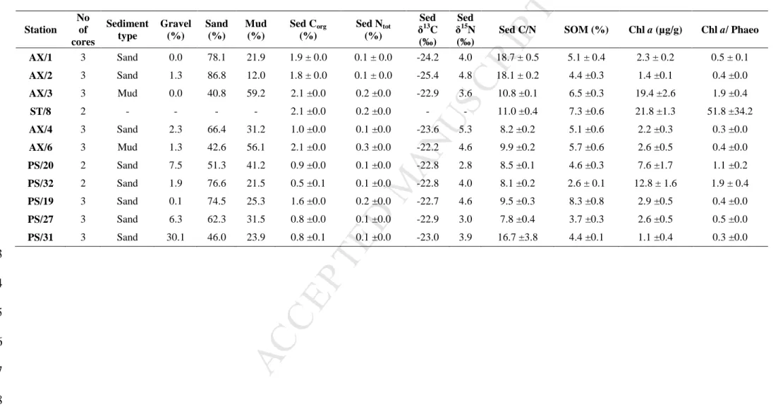
10.3 ± 1.2) (Table 2). Sandy and muddy sediments dominated in the study area. The lowest 365
SOM concentrations were measured at station PS/32, on slope (2.6% ± 0.1) and the highest in 366
Storfjorden (AX/3; 6.5% ± 0.3). The most depleted sediment δ13C values occurred in fjords 367
(AX/1: -24.2‰ and AX/2: -25.4‰) while the most enriched values were found on southern 368
Barents Sea shelf (AX/6: -22.2‰). The lowest Sed C/N ratio values were found in deep basin 369
(PS/27: 7.8 ± 0.4) and the highest value occurred in Van Mijenfjorden (AX/1: 18.7 ± 0.5) 370
(Table 3). 371
M
AN
US
CR
IP
T
AC
CE
PT
ED
19Table 2. Bottom water (BW) characteristics for each sampling station: Corg, Ntot, δ13C, δ15N (in %) and C/N values (mean ± SD, n=3). 372 373 374 375 376 377 378 379 380
Station BW Corg (%) BW Ntot (%) BW δ13C (‰) BW δ15N(‰) BW C/N
AX/1 0.204±0.017 0.023±0.002 -24.7±0.1 5.7±0.7 10.3±1.1 AX/2 0.187±0.005 0.024±0.001 -24.0±0.1 3.9±0.5 8.9±0.2 AX/3 0.630±0.037 0.097±0.005 -22.2±0.2 4.8±0.3 7.6±0.2 ST/8 - - - - - AX/4 0.137±0.047 0.015±0.003 -24.0±0.1 5.1±0.2 10.2±1.7 AX/6 0.268±0.013 0.031±0.005 -24.5±0.9 5.9±1.7 10.3±1.2 PS/20 0.354±0.017 0.063±0.001 -23.5±0.0 1.4±0.0 6.6±0.2 PS/32 0.180±0.002 0.030±0.001 -27.7±0.1 1.9±0.6 7.0±0.2 PS/19 0.188±0.014 0.032±0.001 -24.6±0.2 2.1±0.2 6.8±0.2 PS/27 0.226±0.007 0.040±0.001 -22.9±0.2 2.0±0.7 6.6±0.1 PS/31 0.258±0.013 0.050±0.002 -23.8±0.1 2.3±0.7 6.1±0.0
M
AN
US
CR
IP
T
AC
CE
PT
ED
20Table 3. Sediment variables for each sampling station: sediment type, Corg, Ntot, δ13C, δ15N, OM (in %), C/N, Chl a (µg DW g-1) and Chl a/Phaeo 381
values (mean ± SD, n=no of cores).
382 Station No of cores Sediment type Gravel (%) Sand (%) Mud (%) Sed Corg (%) Sed Ntot (%) Sed δ13C (‰) Sed δ15N (‰)
Sed C/N SOM (%) Chl a (µg/g) Chl a/ Phaeo AX/1 3 Sand 0.0 78.1 21.9 1.9 ± 0.0 0.1 ± 0.0 -24.2 4.0 18.7 ± 0.5 5.1 ± 0.4 2.3 ± 0.2 0.5 ± 0.1 AX/2 3 Sand 1.3 86.8 12.0 1.8 ± 0.0 0.1 ± 0.0 -25.4 4.8 18.1 ± 0.2 4.4 ±0.3 1.4 ±0.1 0.4 ±0.0 AX/3 3 Mud 0.0 40.8 59.2 2.1 ±0.0 0.2 ±0.0 -22.9 3.6 10.8 ±0.1 6.5 ±0.3 19.4 ±2.6 1.9 ±0.4 ST/8 2 - - - - 2.1 ±0.0 0.2 ±0.0 - - 11.0 ±0.4 7.3 ±0.6 21.8 ±1.3 51.8 ±34.2 AX/4 3 Sand 2.3 66.4 31.2 1.0 ±0.0 0.1 ±0.0 -23.6 5.3 8.2 ±0.2 5.1 ±0.6 2.2 ±0.3 0.3 ±0.0 AX/6 3 Mud 1.3 42.6 56.1 2.1 ±0.0 0.3 ±0.0 -22.2 4.6 9.9 ±0.2 5.7 ±0.6 2.6 ±0.5 0.4 ±0.0 PS/20 2 Sand 7.5 51.3 41.2 0.9 ±0.0 0.1 ±0.0 -22.8 2.8 8.5 ±0.1 4.6 ±0.3 7.6 ±1.7 1.1 ±0.2 PS/32 2 Sand 1.9 76.6 21.5 0.5 ±0.1 0.1 ±0.0 -22.8 4.0 8.1 ±0.2 2.6 ± 0.1 12.8 ± 1.6 1.9 ± 0.4 PS/19 3 Sand 0.1 74.5 25.3 1.6 ±0.0 0.2 ±0.0 -22.7 4.6 9.5 ±0.3 8.3 ±0.8 2.9 ±0.5 0.4 ±0.0 PS/27 3 Sand 6.3 62.3 31.5 0.8 ±0.0 0.1 ±0.0 -22.9 3.0 7.8 ±0.4 3.7 ±0.3 2.6 ±0.5 0.5 ±0.0 PS/31 3 Sand 30.1 46.0 23.9 0.8 ±0.1 0.1 ±0.0 -23.0 3.9 16.7 ±3.8 4.4 ±0.1 1.1 ±0.4 0.3 ±0.0 383 384 385 386 387 388
M
AN
US
CR
IP
T
AC
CE
PT
ED
213.2. Macrobenthic community structure
389 390
In total, 186 taxa were identified. The number of taxa per station ranged from 9 (AX/2) 391
to 68 (PS/32) (Table 4). Four burrowing and four sediment-mixing types were recorded. Sub-392
surface burrowing, Cirratulidae (biodiffusor) and Lumbrineris sp. (gallery diffusor) dominated 393
in Svalbard fjords in biomass and density, and in Storfjorden in density. The deep burrowing 394
Yoldia hyperborea (conveyor) dominated in biomass at AX/3. Two biodiffusors, the tube
395
building polychaete Myriochele heeri and the deep burrowing bivalve Astarte borealis 396
dominated in Erik Eriksen station (AX/4) in density and biomass respectively. The tube 397
building Spiochaetopterus typicus (conveyor) dominated in terms of density and was second 398
dominant in biomass in the Southern Barents Sea (AX/6). The sea star Ctenodiscus sp. 399
dominated in biomass at this station. The tube building polychaete, Maldane glebifex, 400
dominated in both density and biomass at the shelf station PS/20. Deep burrowing bivalves 401
(Yoldiella lenticula, Yoldia hyperborea) dominated in density at PS/32 while the tube building 402
polychaete Galathowenia oculata dominated in biomass. Burrow-building taxa were mostly 403
biodiffusors and dominated at all shallow stations. Deep burrowing and tube building taxa 404
were mostly conveyor bioturbators and dominated at deeper stations (Table 4). Fourteen 405
mobility-feeding groups were recorded, and sessile and mobile macrofauna dominated at all 406
stations except from the deepest one (PS/31) where discretely mobile fauna dominated. The 407
lowest number of functional groups was found in Hornsund (AX/2) where 4 groups (sessile 408
surface feeders, discretely subsurface feeders, mobile omnivore and mobile subsurface 409
feeders) occurred. Sessile subsurface feeders dominated at PS/20 (30%) and PS/27 (33%). 410
Sessile surface feeders were predominant in fjords (AX/1: 52% ; AX/2: 80%), Storfjorden 411
(AX/3: 35%), in the southern Barents Sea (AX/6: 45%) and on slope (PS/19: 18%). The share 412
of discretely mobile fauna increased with depth, and discretely mobile surface feeders 413
M
AN
US
CR
IP
T
AC
CE
PT
ED
22dominated in the Nansen Basin (PS/31: 44%). The highest number of mobile subsurface 414
feeders was found on the shelf (PS/32: 23%). The number of mobile taxa was similar for all 415
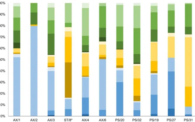
stations. The mobile surface fauna dominated in Erik Eriksen Strait (AX/4: 25%) (Fig. 2). 416 417 418 419 420 421 422 423 424 425 426 427 428 429 430 431 432 433 434 435 436 437 438 439 440
M
AN
US
CR
IP
T
AC
CE
PT
ED
23Table 4. Functional traits, relative density and biomass of the three dominant taxa for each sampling station. Class: P – Polychaeta, B – Bivalvia,
441
An – Anthozoa, As – Asteroidea, O – Ophiuroidea, S – Sipunculidea. Mobility and feeding groups (M/F) are marked by codes: mobility type (D -
442
Discretely mobile, M – Mobile, S – Sessile) and feeding type (car - carnivore, omn - omnivore, sub - subsurface feeder, sur - surface feeder, sus -
443
suspension feeder). Burrowing depth (BT): 1 – surface burrowing, 2 – subsurface burrowing, 3 – deep burrowing. Tubes (T): “+” – I-shaped
444
tube, “-“ – no tube. Sediment mixing types (SMix): biodiffusor (B), upward conveyor (UC), gallery diffusor (GD), downward conveyor (DC).
445
Station No
of taxa
Taxa Class M/F BT T SMix Density
% Taxa Class M/F BT T SMix
Biomass % AX/1 20 Cirratulidae 2 P Ssur 2 - B 41.4 Lumbrineris sp. 6 P Momn 2 - GD 72.1
Polycirrus arcticus 4,5 P Ssur 3 + DC 7.1 Polycirrus arcticus 4,5 P Ssur 3 + DC 11.5
Lumbrineris sp. 6 P Momn 2 - GD 6.4 Aglaophamus malmgreni 4 P Mcar 2 - B 10.6
AX/2 9 Cirratulidae 2 P Ssur 2 - B 66.7 Cirratulidae 2 P Ssur 2 - B 49.3
Polycirrus arcticus 4,5 P Ssur 3 + DC 13.1 Polycirrus arcticus 4,5 P Ssur 3 + DC 36.6
Lumbrineris sp. 6 P Momn 2 - GD 8.3 Lumbrineris sp. 6 P Momn 2 - GD 8.7
AX/3 34 Cirratulidae 2 P Ssur 2 - B 31.2 Yoldia hyperborea 7 B Msub 3 - C 57.4
Lumbrineris sp. 6 P Momn 2 - GD 14.1 Maldane sarsi 8 P Ssub 3 + C 12
Yoldia hyperborea 7 B Msub 3 - C 6.3 Nuculana radiata 4 B Msub 3 - B 11.5
ST/8 29 Lumbrineris sp. 6 P Momn 2 - GD 18.3 Yoldia hyperborea 7 B Msub 3 - C 30.5
Cirratulidae 2 P Ssur 2 - B 11 Nuculana radiata 4 B Msub 3 - B 27.8
Eteone longa 9, 10 P Msub 1 - GD 7.3 Macoma calcarea 11 B Ssur 3 - B 13.7
M
AN
US
CR
IP
T
AC
CE
PT
ED
24Macoma sp. 1, 11 B Ssur 3 - B 11.6 Actinaria 4 An Scar 1 - B 1.8
Maldane sarsi 8 P Ssub 3 + C 8.2 Yoldiella lenticula 7 B Msur 3 - C 1.5
AX/6 36 Spiochaetopterus typicus 8 P Ssur 3 + C 34.9 Ctenodiscus sp. 20 As Msur 1 - B 47.3
Macoma sp. 1, 11 B Ssur 3 - B 6.4 Spiochaetopterus typicus 8 P Ssur 3 + C 27.3
Heteromastus sp. 12, 13, 14 P Msub 3 - C 6.4 Aglaophamus malmgreni 4 P Mcar 2 - B 6.4
PS/20 58 Maldane glebifex 8 P Ssub 3 + C 22.4 Maldane glebifex 8 P Ssub 3 + C 24.5
Yoldiella lenticula 7 B Msur 3 - C 8.7 Chirimia biceps 8 P Ssub 3 + C 9.4
Macoma calcarea 11 B Ssur 3 - B 7.1 Nicomache lumbricalis 8 P Ssub 3 + C 9.4
PS/32 68 Yoldiella lenticula 7 B Msur 3 - C 13.8 Galathowenia oculata 3 P Msur 2 + C 7.7
Yoldia hyperborea 7 B Msub 3 - C 8.7 Ctenodiscus sp. 20 As Msur 1 - B 7.5
Axinopsida orbiculata 15 B Dsub 3 - C 5.9 Yoldiella lenticula 7 B Msur 3 - C 6.3
PS/19 38 Cirratulidae 2 P Ssur 2 - B 12 Amphiura sundevalli 4 O Msus 1 - B 25.5
Notoproctus oculatus 8 P Ssub 3 + C 10.1 Lumbrineridae 6 P Somn 2 - GD 9.3
Yoldia hyperborea 7 B Msub 3 - C 8.9 Nemertea 4 N Momn 1 - B 7.1
PS/27 35 Prionospio cirrifera 16 P Dsur 2 + C 13.2 Streblosoma intestinale 4 P Dsur 3 + C 43
Notoproctus oculatus 8 P Ssub 3 + C 13.2 Chone fauveli 3 P Ssur 2 + C 32.6
Lumbriclymene minor 8 P Ssub 3 + C 8.8 Notoproctus oculatus 8 P Ssub 3 + C 4.2
PS/31 19 Levinsenia gracilis 18 P Dsur 2 - C 33.6 Nephasoma lilljeborgi 19 S Dsur 3 - C 28
Paraonidae 2 P Msub 2 - B 19.3 Levinsenia gracilis 18 P Dsur 2 - C 14.2
Cirrophorus sp. 2 P Dsub 2 - B 16.8 Paraonidae 2 P Msub 2 - B 11 446
M
AN
US
CR
IP
T
AC
CE
PT
ED
25References in superscripts: 1 Gilbert at al. (2007); 2 Gérino at al. (1992, 2007); 3 Fauchald and Jumars (1979); 4 Queirós at al. (2013); 5 Gingras et
447
al. (2008); 6 Petch (1986); 7 Stead and Thompson (2006); 8 Smith and Shafer (1984); 9 Mazik and Elliott (2000); 10 Mermillod-Blondin et al.
448
(2003); 11 Michaud et al. (2006); 12 D'Andrea et al. (2004); 13 Mulsow et al. (2002); 14 Quintana et al. (2007); 15 Zanzerl and Dufour (2017); 16
449
Bouchet et al. (2009); 17 Duchêne and Rosenberg (2001); 18 Venturini et al. (2011); 19 Shields and Kędra (2009); 20 Shick (1976).
M
AN
US
CR
IP
T
AC
CE
PT
ED
26 451 452Fig. 2. Percentages of mobility and feeding groups at different sampling stations. Station ST/8 453
marked with * was sampled in summer season. Functional traits codes: mobility type (D - 454
Discretely mobile (yellow), M – Mobile (green), S – Sessile (blue)) and feeding type (car - 455
carnivore, omn - omnivore, sub - subsurface feeder, sur - surface feeder, sus - suspension 456
feeder). 457
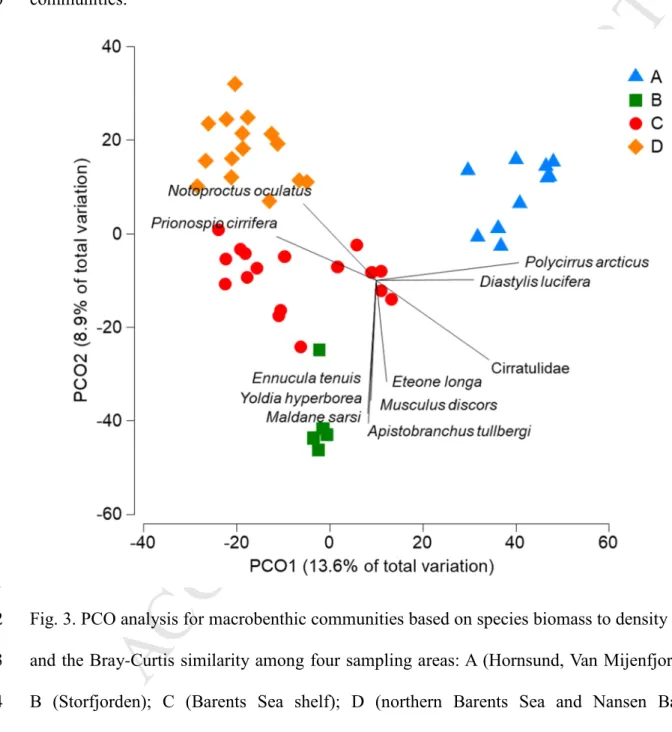
Stations were separated into 4 groups, based on the PCO analysis: A - fjords (Van 458
Mijenfjorden: AX/1, Hornsund: AX/2), B - Storfjorden (AX/3), C - Barents Sea shelf (Erik 459
Eriksen Strait: AX/4, southern Barents Sea: AX/6, and northern Barents Sea: PS/20, PS/32), D 460
- northern Barents Sea, stations deeper than 400m on continental stock: PS/19, PS/27 and 461
Nansen Basin: PS/31. PCO explained 22.5% of the variability among sampling stations: the 462
first axis explained 13.6% and the second axis 8.9% (Fig. 3). Fjords’ communities were 463
correlated with presence of polychaete Polycirrus arcticus and cumacean Diastylis lucifera 464
while benthic patterns in Storfjorden were correlated with presence of polychaetes Maldane 465
M
AN
US
CR
IP
T
AC
CE
PT
ED
27sarsi and Apistobranchus tullbergi, and bivalves Musculus discors, Ennucula tenuis and
466
Yoldia hyperborea. Those correlations were negative for deeper stations where benthic
467
communities were mainly correlated with presence of polychaetes Notoproctus oculatus and
468
Prionospio cirrifera. The shelf stations varied the most with less clear patterns for benthic
469
communities.
470
471
Fig. 3. PCO analysis for macrobenthic communities based on species biomass to density ratio,
472
and the Bray-Curtis similarity among four sampling areas: A (Hornsund, Van Mijenfjorden);
473
B (Storfjorden); C (Barents Sea shelf); D (northern Barents Sea and Nansen Basin).
474
Significantly correlated species with the PCO coordinates (r>0. 5) are shown on the plot.
475 476
M
AN
US
CR
IP
T
AC
CE
PT
ED
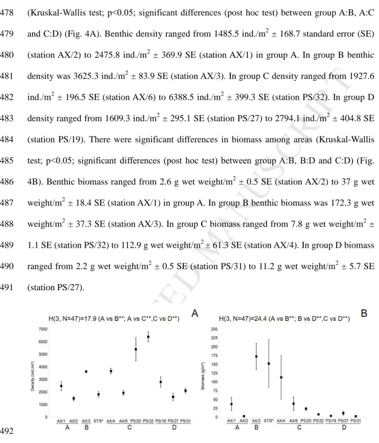
28Polychaeta dominated at all stations. There were significant differences in density 477
(Kruskal-Wallis test; p<0.05; significant differences (post hoc test) between group A:B, A:C 478
and C:D) (Fig. 4A). Benthic density ranged from 1485.5 ind./m2 ± 168.7 standard error (SE) 479
(station AX/2) to 2475.8 ind./m2 ± 369.9 SE (station AX/1) in group A. In group B benthic 480
density was 3625.3 ind./m2 ± 83.9 SE (station AX/3). In group C density ranged from 1927.6 481
ind./m2 ± 196.5 SE (station AX/6) to 6388.5 ind./m2 ± 399.3 SE (station PS/32). In group D 482
density ranged from 1609.3 ind./m2 ± 295.1 SE (station PS/27) to 2794.1 ind./m2 ± 404.8 SE 483
(station PS/19). There were significant differences in biomass among areas (Kruskal-Wallis 484
test; p<0.05; significant differences (post hoc test) between group A:B, B:D and C:D) (Fig.
485
4B). Benthic biomass ranged from 2.6 g wet weight/m2 ± 0.5 SE (station AX/2) to 37 g wet 486
weight/m2 ± 18.4 SE (station AX/1) in group A. In group B benthic biomass was 172.3 g wet 487
weight/m2 ± 37.3 SE (station AX/3). In group C biomass ranged from 7.8 g wet weight/m2 ± 488
1.1 SE (station PS/32) to 112.9 g wet weight/m2 ± 61.3 SE (station AX/4). In group D biomass 489
ranged from 2.2 g wet weight/m2 ± 0.5 SE (station PS/31) to 11.2 g wet weight/m2 ± 5.7 SE 490
(station PS/27). 491
492
Fig. 4. Mean density (ind./m-2) (A) and biomass (g/m-2) (B); ± SE, n= no of cores (Table 1) at 493
stations sampled in Van Mijenfjorden, Hornsund (group A); Storfjorden (group B); Barents
494
Sea shelf (group C); northern Barents Sea and Nansen Basin (group D). Station ST/8 marked 495
M
AN
US
CR
IP
T
AC
CE
PT
ED
29with * was sampled in summer season. Kruskal – Wallis results for differences between 496
sampling sites are given; significant test results are marked with ** (p<0.05).
497
There were significant differences in the benthic communities structure 498
(biomass/density ratio) among different locations (PERMANOVA test Pseudo-F : 5.07, 499
p=0.001). Significant differences were found for each group (significant pairwise 500
comparisons p=0.001); see Table 5 for details. 501
502
Table 5. PERMANOVA results for the multivariate descriptors of benthic communities with 503
significant pair-wise comparisons results for different groups. 504
Benthic parameter Source of variation Df MS Pseudo-F P (perm)
Biomass/Density ratio Gr 3 16606.0 5.07 0.001
Res 43 3272.8
Total 46
Benthic parameter Regime Site t Df P(MC) P (perm)
Biomass/Density ratio Groups A:B 2.886 13 0.001 0.001
A:C 2.469 25 0.001 0.001 A:D 2.715 23 0.001 0.001 B:C 1.874 20 0.001 0.001 B:D 2.151 18 0.001 0.001 C:D 1.852 30 0.001 0.001 505 506
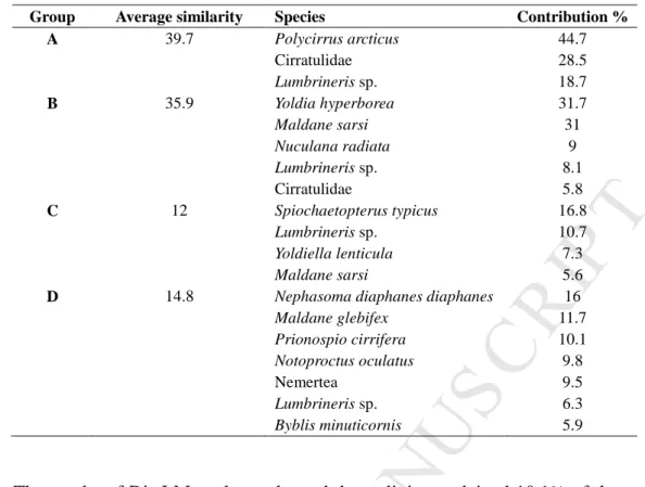
Benthic taxa that contributed mostly to the groups similarities were: Polycirrus 507
arcticus (44.7 %) in fjords (A), Yoldia hyperborea (31.7 %) in Storfjorden (B), 508
Spiochaetopterus typicus (16.8 %) in the Barents Sea shelf (C) and Nephasoma diaphanes
509
diaphanes(16 %) in the northern Barents Sea and Nansen Basin (D) as revealed by SIMPER 510
analysis (Table 6). 511
512
Table 6. SIMPER analysis results based on B/D ratio. Species that contributed more than 5% 513
of the average similarity for different sampling stations groups are listed. 514
M
AN
US
CR
IP
T
AC
CE
PT
ED
30Group Average similarity Species Contribution %
A 39.7 Polycirrus arcticus 44.7 Cirratulidae 28.5 Lumbrineris sp. 18.7 B 35.9 Yoldia hyperborea 31.7 Maldane sarsi 31 Nuculana radiata 9 Lumbrineris sp. 8.1 Cirratulidae 5.8 C 12 Spiochaetopterus typicus 16.8 Lumbrineris sp. 10.7 Yoldiella lenticula 7.3 Maldane sarsi 5.6
D 14.8 Nephasoma diaphanes diaphanes 16
Maldane glebifex 11.7 Prionospio cirrifera 10.1 Notoproctus oculatus 9.8 Nemertea 9.5 Lumbrineris sp. 6.3 Byblis minuticornis 5.9 515
The results of DistLM analyses showed that salinity explained 10.1% of the variation 516
observed in the macrofauna community while Sed δ13C (10%) and Sed C/N (9.3%) were next 517
main contributors. Nine variables were included by the DistLM procedure to construct the 518
best fitting model, together explaining 46.8% of total variation. However, one of the variables 519
was not statistically significant (gravel) (Table 7). The most important parameter contributing 520
to the first axis of the dbRDA plot was Sed C/N and explained 17.2% of fitted variation. It 521
also positively correlated with fjords’ group (A). The most important parameter contributing 522
to the second axis was sediment Chl a and explained 25.7% of fitted flux variation. It was 523
positively correlated with Storfjords group (B) and most stations in group C (shelf) (Fig. 5). 524
525
Table 7. Results of DistLM procedure for fitting environmental variables to the macofauna 526
community data. %Var - percentage of explained variance; %Cum - cumulative percentage 527
explained by the added variable. Significance level p < 0.05. Environmental factors: D – 528
depth, S – salinity, T – temperature, types of sediment (mud, sand, gravel), BW Corg – bottom 529
water Corg, BW Ntot – bottom water Ntot, BW δ13C – bottom water δ13C BW, BW δ15N – 530
M
AN
US
CR
IP
T
AC
CE
PT
ED
31bottom water δ15N, BW C/N – bottom water C/N, Sed Corg – Corg concentration in sediment, 531
Sed Ntot – sediment Ntot, Sed δ13C – sediment δ13C, Sed δ15N – sediment δ15N, Sed C/N – 532
sediment C/N, SOM – sediment organic matter, Chl a – sediment Chlorophyll a and Chl 533
a/Phaeo – sediment Phaeopigments.
534
MARGINAL TESTS
Variable Pseudo-F Var% P
S 5.06 10.1 0.001 Sed δ13C 5.01 10.0 0.001 Sed C/N 4.59 9.3 0.001 BW C/N 4.31 8.7 0.001 BW δ15N 4.25 8.6 0.001 Sed Corg 4.11 8.4 0.001 D 3.99 8.1 0.001 T 3.96 8.1 0.001 Chl a 3.66 7.5 0.001 Sand 3.62 7.4 0.001 Mud 3.46 7.1 0.001 Chl a/ Phaeo 3.34 6.9 0.001 BW Corg 3.26 6.8 0.001 BW Ntot 3.16 6.6 0.002 Gravel 3.11 6.5 0.001 Sed Ntot 2.43 5.1 0.001 Sed δ15N 2.09 4.4 0.004 BW δ13C 2.04 4.3 0.001 SOM 1.56 3.4 0.032 SEQUENTIAL TESTS
Variable R² Pseudo-F Var% Cum% P
D 0.08 3.99 8.1 8.1 0.001 S 0.16 3.98 7.6 15.7 0.001 Sand 0.30 4.06 7.0 22.7 0.001 BW δ15N 0.44 3.71 5.5 28.2 0.001 BW C/N 0.49 3.70 5.1 33.3 0.001 BW δ13C 0.38 3.06 4.9 38.1 0.001 T 0.20 2.44 4.5 42.7 0.001 Mud 0.33 2.26 3.8 46.4 0.001 Gravel 0.23 1.29 2.4 48.8 0.127 535
M
AN
US
CR
IP
T
AC
CE
PT
ED
32 536Fig. 5. Distance-based Redundancy Analysis (dbRDA) plot of the DistLM model visualizing
537
the relationships between the environmental parameters and the biomass/density ratio of
538
species between four sampling areas: A (Hornsund, Van Mijenfjorden); B (Storfjorden); C
539
(Barents Sea shelf); D (northern Barents Sea and Nansen Basin). Environmental variables
540
with Pearson rank correlations with dbRDA axes > 0.5 are shown. Environmental factors: D –
541
depth, S – salinity, T – temperature, types of sediment (mud, sand, gravel), BW Corg – bottom 542
water Corg, BW Ntot – bottom water Ntot, BW δ15N – bottom water δ15N, BW C/N – bottom 543
water C/N, Sed Corg – Corg concentration in sediment, Sed δ13C – sediment δ13C, Sed C/N – 544
sediment C/N, Chl a – sediment Chlorophyll a and Chl a/Phaeo – sediment Phaeopigments.
545 546
3.3.Bioturbation
M
AN
US
CR
IP
T
AC
CE
PT
ED
33 548After 10 days, almost all luminophores (~95%) remained on sediment core surface at all 549
sampling stations meaning that about 5% of luminophores were transported into sediments. 550
The fastest decrease was noted at the B group (Storfjorden : AX/3 and ST/8), and at the C 551
group (Southern Barents Sea station (AX/6) ; Nansen Basin < 400 m (PS/20, PS/32)) where 552
~15 to 25% of surface luminophores were buried. While luminophores were still present all 553
along the sedimentary column in the Storfjorden station, some subsurface peaks of 554
luminophores were clearly measured below 3 cm in the C group. The lowest decrease of the 555
luminophores over depth was noted in the A group (Svalbard Fjords AX1/1, AX/2) and in the 556
D group at deepest station (PS/31) in the Nansen Basin where 92 to 98% of luminophores 557
remained at surface with slight subsurface peaks of tracers (about: only 0.91 %) between 1 to 558
3 cm deep . 559
Biodiffusion rates ranged from 0.04 cm-2 y-1 ± 0.01 standard error (SE) (station AX/2) 560
to 0.07 cm-2 y-1 ± 0.03 SE (station AX/1) in group A. In group B biodiffusion rates was 0.06 561
cm-2 y-1 ± 0.04 SE (station AX/3). In group C biodiffusion ranged from 0 (station PS/32) to 562
0.76 cm-2 y-1 ± 0.71 SE (station AX/6). There was no biodiffusive transport in group D. There 563
were significant differences in biodiffusion among areas (Kruskal-Wallis test; p<0.05; 564
significant differences (post hoc test) between group A:D and C:D) (Fig. 6A). Non-local 565
transport rates ranged from 0.21 y-1 ± 0.20 SE (station AX/2) to 0.60 y-1 ± 0.23 SE (station 566
AX/1) in group A. In group B non-local transport rates was 2.12 y-1 ± 1 SE (station AX/3). In 567
group C non-local transport rates ranged from 0.75 y-1 ± 0.25 SE (station PS/32) to 2.08 y-1 ± 568
0.58 SE (station AX/6). In group D non-local transport rates ranged from 0.28 y-1 ± 0.04 SE 569
(station PS/31) to 0.68 y-1 ± 0.31 SE (station PS/19). There were significant differences in 570
non-local transport (Kruskal-Wallis test; p<0.05; significant differences (post hoc test) 571
between group A:C and C:D) (Fig. 6B). Biodiffusive transport values were significantly 572
M
AN
US
CR
IP
T
AC
CE
PT
ED
34related with depth, Sed Corg and BW C/N ratio Spearman correlation: -0.6, 0.6 and 0.6, p<0.05 573
respectively). Non-local transport values were significantly related to benthic taxa richness, 574
biomass, mud and Sed Ntot (Spearman correlation: 0.5, 0.5, 0.5 and 0.5 p<0.05 respectively) 575
(Table 8). 576
577
Fig. 6. Mean bioturbation coefficients: Db - biodiffusion (cm-2 y-1) (A) and r – non-local (y-1) 578
(B); ± SE, n=no of cores (Table 1) at stations sampled in Van Mijenfjorden, Hornsund (group 579
A); Storfjorden (group B); Barents Sea shelf (group C); northern Barents Sea and Nansen
580
Basin (group D). Station ST/8 marked with * was sampled in summer season. Kruskal – 581
Wallis results for differences between sampling sites are given; significant test results are 582
marked with ** (p<0.05). 583
M
AN
US
CR
IP
T
AC
CE
PT
ED
35Table 8. Spearman’s rank correlation analyses among biological and physical parameters. Significant values are marked in bold (p<0.05).
584 N o o f ta x a D en si ty B io m a ss N o n -l o ca l (r ) B io d if fu si o n ( D b ) D ep th S a li n it y T em p er a tu re G ra v el S a n d M u d B W C o rg B W N to t B W δ 1 3 C B W δ 1 5 N B W C /N S ed C o rg S ed N to t S ed δ 1 3 C S ed δ 1 5 N S ed C /N S O M C h l a C h l a /P h a eo No of taxa - 0.9 0.5 0.5 0.0 -0.1 0.2 0.1 0.0 -0.1 0.3 -0.1 0.0 -0.1 -0.2 0.0 -0.2 0.3 0.5 -0.1 -0.6 0.1 0.6 0.2 Density 0.9 - 0.5 0.4 -0.1 -0.2 -0.1 0.0 0.0 -0.1 0.2 -0.1 0.1 -0.1 -0.2 -0.1 -0.2 0.1 0.3 -0.1 -0.3 0.1 0.5 0.3 Biomass 0.5 0.5 - 0.5 0.4 -0.5 -0.2 -0.3 -0.3 -0.4 0.6 0.3 0.0 0.2 0.4 0.4 0.4 0.6 0.2 -0.1 -0.1 0.3 0.4 0.3 Non-local (r) 0.5 0.4 0.5 - 0.3 -0.2 0.1 0.0 -0.1 -0.4 0.5 0.2 0.1 0.1 0.2 0.2 0.2 0.5 0.4 -0.1 -0.3 0.3 0.4 0.1 Biodiffusion (Db) 0.0 -0.1 0.4 0.3 - -0.6 -0.4 -0.3 -0.3 0.0 0.2 0.2 -0.2 0.0 0.5 0.6 0.6 0.4 -0.2 0.2 0.4 0.3 0.0 0.0 585
M
AN
US
CR
IP
T
AC
CE
PT
ED
363.4. Storfjorden – seasonal changes
586 587
Bottom water salinity was similar in spring and summer in Storfjorden, respectively 588
34.5 and 34.1. Bottom water temperature in spring season was -0.8 °C and increased to 4.5 °C 589
(Table 1). Benthic density decreased from 3625.3 ind./m2 ± 83.9 SE in spring (AX/3) to 590
1812.7 ind./m2 ± 229.7 SE in summer (ST/8). Biomass was similar in both seasons (172.3 591
g/m2 ± 37.3 SE (spring, AX/3) and 152.1 g/m2 ± 67.5 SE (summer, ST/8). Non-local transport 592
rates were similar in spring and summer (2.12 ± 1 and 2.09 ± 0.72 y-1 respectively) but 593
biodiffusion rates increased in summer (0.06 ± 0.04 in spring and 0.90 ± 0.90 cm2 y-1 in 594
summer). Significant differences were found for the number of taxa and macrofauna density 595
between spring and summer seasons (Mann-Whitney U-test; Z= 2.3; p<0.05 and Z=2.4; 596 p<0.05, respectively). 597 598 4. Discussion 599 600
This is the first complex report on bioturbation activities in spring to summer 601
transition time conducted over the large area from Svalbard fjords and Barents Sea to deep 602
basin north off Svalbard. In our study, benthic community variables differentiated four 603
groups of stations, and this separation was to some extent echoed by the environmental 604
factors. The benthic community properties further affected the measured benthic activities i.e. 605
bioturbation rates. 606
607
4.1. Benthic community characteristics across the sampled area 608