An adaptive finite element solution algorithm for the Euler equations

An Adaptive Finite Element Solution

Algorithm for the Euler Equations

by

Richard Abraham Shapiro

S.B. Mathematics, Massachusetts Institute of Technology, 1983

S.B. Aeronautics and Astronautics, Massachusetts Institute of Technology, 1983 S.M. Aeronautics and Astronautics, Massachusetts Institute of Technology, 1984

SUBMITTED IN PARTIAL FULFILLMENT OF THE REQUIREMENTS FOR THE DEGREE OF

Doctor of Philosophy

in

Computational Fluid Dynamics

Department of Aeronautics and Astronautics

at the

Massachusetts Institute of Technology

May 1988

@1988, Massachusetts Institute of Technology

Signature of Author

Departmypt of Aeronautics and Astronautics Certified by

Professof Earll M. Murman

Thesis Supervisor, Department Lutics

Certified by

Professor Michael B. Giles Certified by

Professor Lloyd N. Trefethen Accepted by

Pr(essor Harold Y. Wachman Chairman, Department Graduate Committee

SWiTHDI•A

WN

'MAY

_{2 4 1988}

_M.i.T.

An Adaptive Finite Element Solution Algorithm for the

Euler Equations

by

Richard Abraham Shapiro

Submitted to the Department of Aeronautics and Astronautics, April 29, 1988 in partial fulfillment of the requirements for the degree of

Doctor of Philosophy in Computational Fluid Dynamics

A new finite element algorithm for solving the steady Euler equations describing the flow

of an inviscid, compressible, ideal gas is presented. This algorithm uses a finite element spatial discretization coupled with a Runge-Kutta time integration to relax to steady state. It is shown that other algorithms, such as finite difference and finite volume methods, can be derived using finite element principles. A higher-order biquadratic ap-proximation is introduced. Several test problems are computed to verify the algorithms. Adaptive gridding in two and three dimensions using quadrilateral and hexahedral el-ements is developed and verified. Adaptation is shown to provide CPU savings of a factor of 2-16, and biquadratic elements are shown to provide potential savings of a factor of 2-6. An analysis of the dispersive properties of various discretization methods for the Euler equations is presented, and results allowing the prediction of dispersive errors are obtained. The adaptive algorithm is applied to the solution of several flows in scramjet inlets in two and three dimensions, demonstrating some of the varied physics associated with these flows. Some issues in the design and implementation of adaptive finite element algorithms on vector and parallel computers are discussed.

Acknowledgements

Many people have contributed to this research over the years, and I am very grateful

for all the help I have received.

Professors Earll Murman, Mike Giles, Lloyd N. Trefethen, and Saul Abarbanel have

provided many insights into the fluid mechanical problems and the mathematics behind

their solution. Special thanks go to my advisor Prof. Murman, for helping me with

more sticky problems than I'd care to remember.

I also want to thank Dr. Rainald L6hner, Prof. Ken Morgan and Prof. Earl Thornton

for all the ideas, conversations and criticisms they provided.

My colleagues in the CFL lab have been wonderful foils for ideas and helpful in

pointing out the obvious (and not-so-obvious) problems in any research effort. I'd

especially like to recognize Dr. John Dannenhoffer, Prof. Ken Powell, Dr. Tom Roberts,

Steve Allmaras and Dana Lindquist for their many helpful suggestions and much useful

advice. I also want to thank Dave Modiano for his work on a three-dimensional plot

package which made debugging the 3-D, adaptive code possible.

In Computational Fluid Dynamics, not much would happen if there were no

com-puters. Thanks to Bob Bruen and Teva Regule for keeping the computers at home

crunching away. Special thanks also go to Gerry Cocco and Corey Lowen from IBM

for their efforts in getting the supercomputer time at Cornell, and then spending many

late hours teaching me how to use it.

I thank my family for encouragement throughout my time at MIT. Most of all, I

want to thank my wife Heather for helping me keep things in perspective and for all her

support throughout the time I've been a graduate student. Her contributions to this

thesis, direct and indirect, I will treasure always.

This work was supported in part by the Air Force Office of Scientific Research under

contracts AFOSR-87-0218 and AFOSR-82-0136, and in part by the Fannie and John

Hertz Foundation.

Trust in the LORD with all thine heart; and lean not unto thine own under-standing. In all thy ways acknowledge him, and he will direct thy paths.

-Proverbs 3:5,6

I can do all things through Christ which strengtheneth me.

Contents

Acknowledgements

1 Introduction

1.1 Research Goals ...

1.2 Overview of Thesis ...

1.3 raggedright Survey of Finite Element Methods for the Euler Equations .

2 Governing Equations

2.1 Euler Equations ...

2.2 Non-Dimensionalization of the Equations . . . .

2.3 Auxiliary Quantities ...

2.4 Boundary Conditions ...

2.4.1 Solid Surface Boundary Conditions . . . .

2.4.2 Open Boundary Conditions . . . .

3 Finite Element Fundamentals

3.1 Basic Definitions ...

3.2 Finite Elements and Natural Coordinates . . . .

3.2.1

Properties of Interpolation Functions . . . .

3.2.2 Natural Coordinates and Derivative Calculation . . . .

3.3 Typical Elements . . ...

3.3.1

Bilinear Element ...

22

22

24

25

26

26

26

28

28

31

32

33

34

35

3.3.2 Biquadratic Element ... 37

3.3.3 Trilinear Element ... ... 38

4 Solution Algorithm 41 4.1 Overview of Algorithm ... 41

4.2 Spatial Discretization .. ... .... ... ... . 42

4.3 Choice of Test Functions ... 45

4.3.1 Test Functions for Galerkin Method . . ... 45

4.3.2 Test Functions for Cell-Vertex Method . ... 48

4.3.3 Test Functions for Central Difference Method. .... . . . . . 49

4.4 Boundary Conditions ... 52

4.4.1 Solid Surface Boundary Condition . ... 52

4.4.2 Open Boundary Condition ... 53

4.5 Smoothing ... ... ... . 55

4.5.1 Conservative, Low-Accuracy Second Difference . ... 55

4.5.2 Non-Conservative, High-Accuracy Second Difference ... 56

4.5.3 Combined Smoothing ... 58

4.5.4 Smoothing on Biquadratic Elements . ... 60

4.6 Time Integration ... 60

4.7 Consistency and Conservation ... ... 61

5 Algorithm Verification and Comparisons 63 5.1 Introduction ... 63

5.2 Verification and Comparison of Methods . ... . . . ... 64

5.2.2

15* Converging Channel ...

... .

66

5.2.3 4 % Circular Arc Bump ...

69

5.2.4 10% Circular Arc Bump ...

70

5.2.5 CPU Comparison and Recommendations . ...

70

5.2.6 Verification of Conservation . . . .

71

5.3 Effects of Added Dissipation ...

72

5.4 Biquadratic vs. Bilinear ...

...

73

5.4.1 50 Channel Flow ...

74

5.4.2 4% Circular Arc Bump ...

75

5.4.3 Subsonic, Smooth Flow . . . .

75

5.5 Three Dimensional Verification ...

....

77

5.6 Summary ...

78

6 Adaptation

99

6.1 Introduction ...

99

6.2 Adaptation Procedure ...

101

6.2.1

Placement of Boundary Nodes . ...

103

6.2.2 How Much Adaptation? ...

103

6.3 Adaptation Criteria ...

104

6.3.1

First-Difference Indicator ...

...

105

6.3.2 Second-Difference Indicator

... . . .

106

6.3.3 Two-Dimensional Directional Adaptation . ...

107

6.4 Embedded Interface Treatment ...

....

108

6.4.1 Two-Dimensional Interface ...

..

108

6.5 Examples of Adaptation ...

112

6.5.1

Multiple Shock Reflections ...

...

... .113

6.5.2 4% Circular Arc Bump ...

114

6.5.3

10% Circular Arc Bump ...

115

6.5.4 3-D Channel ...

116

6.5.5 Distorted Grid ...

116

6.6 CPU Time Comparisons ...

...

117

7

Dispersion

Phenomena and the Euler Equations

131

7.1 Introduction ...

...

131

7.2 Difference Stencils ...

132

7.2.1

Some Properties of the Galerkin Stencil . ...

132

7.2.2 Some Properties of the Cell-Vertex Stencil . . . ...

133

7.3 Linearization of the Equations ...

....

134

7.4 Fourier Analysis of the Linearized Equations . ...

136

7.5 Numerical Verification ...

140

7.6 Conclusions ...

142

8 Scramjet Inlets

150

8.1 Introduction...

...

150

8.2 Two-Dimensional Test Cases . . . 151

8.2.1

Moo = 5, 0* Yaw ...

..

152

8.2.2 Moo = 5, 50 Yaw ...

153

8.2.3

Moo = 2, 00 Yaw ...

...

154

8.2.5 Moo = 3, 70 Yaw ...

8.2.6 Inlet Performance and Total Pressure Loss

8.3 Three-Dimensional Results .. . . .

9 Summary and Conclusions 9.1 Summary ...

9.2 Contributions of the Thesis .. . . .

9.3 Conclusions ...

9.4 Areas for Further Exploration .. . . .

A Computational Issues A.1 Introduction ...

A.2 Vectorization and Parallelization Issues .. . . . .

A.3 Computer Memory Requirements .. . . . A.3.1 Two-Dimensional Memory Requirements. A.3.2 Three-Dimensional Memory Requirements.

A.4 Data Structures for Adaptation .. . . .

A.4.1 Finding the Children of an Element . . . . A.4.2 Finding The Adjacent Element .. . . .

B Scramjet Geometry Definition

C Two-Dimensional Code Listings

D Three-Dimensional Code Listings

156 156 157 168 . . . . 168 . . . . . 170 . . . . 171 . . . . . 173 181 181 181 184 184 185 186 187 188 190 192 327

List of Figures

3.1 Example of a General Finite Element Discretization . ... 29

3.2 Definition of Finite Element Terms . . . . 30

3.3 Quadrilateral Element Degenerated into a Triangular Element ... 30

3.4 Geometry of Two-Dimensional Element . ... 35

3.5 Geometry of Three-Dimensional Element . ... 38

4.1 Illustrative Test Functions for Three Methods . . . . 46

4.2 Mesh for Central Difference/Cell-Based Finite Volume Comparison . . . 50

4.3 Two-Dimensional Weights for Second Difference at Node 1. ... 56

4.4 Triangles For Smoothing Calculation ... ... .. . 57

4.5 Integration Polygons for Smoothing Calculation . ... 58

5.1 Convergence History for Failed 15* Wedge, M, = 4 . ... 69

5.2 Geometry for 10* Double Wedge Flow . . . . 76

5.3 Flow Geometry for 50 Channel ... 79

5.4 Coarse Grid, 5* Channel ... ... . 79

5.5 Mach Number, Galerkin, 5* Channel, M=2, 40x10 Grid . ... 79

5.6 Mach Number, Galerkin, 5* Channel, M=2, 80x20 Grid . . . . ... . . 79

5.7 Surface Mach Number, Galerkin, 5* Channel, M=2, 40x10 Grid . . . . . 80

5.8 Surface Mach Number, Galerkin, 5* Channel, M=2, 80x20 Grid .... . 80

5.9 Density Comparison, 5* Channel, M=2, 40x10 Grid, Y=0.6 ... . 81

5.11 Percent Error in Density, 5* Channel, M=2, 40x10 Grid ...

.

82

5.12 Percent Error in Density, 5* Channel, M=2, 80x20 Grid ...

82

5.13 Points with Density Error > 5%, 5* Channel, M=2, 40x10 Grid ...

82

5.14 Points with Density Error > 5%, 5* Channel, M=2, 80x20 Grid ...

82

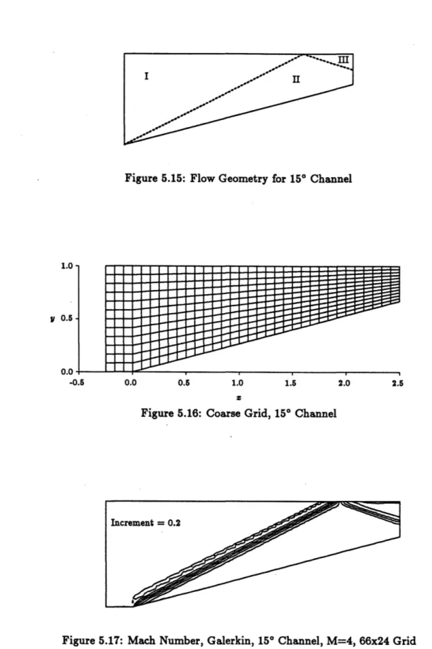
5.15 Flow Geometry for 15* Channel ...

83

5.16 Coarse Grid, 15* Channel ...

83

5.17 Mach Number, Galerkin, 15* Channel, M=4, 66x24 Grid ...

83

5.18 Surface Mach Number, Cell-Vertex, 15* Channel, M=4, 33x12 Grid ... 84

5.19 Surface Mach Number, Cell-Vertex, 15* Channel, M=4, 66x24 Grid ... 84

5.20 Density Comparison, 15* Channel, M=4, 33x12 Grid, Y=0.9 ...

85

5.21 Density Comparison, 15* Channel, M=4, 66x24 Grid, Y=0.9 ...

85

5.22 Points with Density Error > 5%, 15* Channel, M=4, 33x12 Grid . . . . 85

5.23 Points with Density Error > 5%, 15* Channel, M=4, 66x24 Grid . . . . 86

5.24 Pressure Contours, 4% Bump, M,, = 1.4, 60x20 Grid, Galerkin ...

86

5.25 Surface Mach Number, 4% Bump, M = 1.4, 60x20 Grid, Cell-Vertex .

86

5.26 Mid-Channel Density, 4% Bump, M, = 1.4, 60x20 Grid, All Methods .

87

5.27 Pressure, 10% Bump, Moo = 0.68, 60x20 Grid, Galerkin ...

87

5.28 Surface Mach Number, 10% Bump, M, = 0.68, 60x20 Grid, Cell-Vertex

88

5.29 Mid-Channel Density, 10% Bump, M. = 0.68, 60x20 Grid, All Methods

88

5.30 Convergence vs. CPU Time, 4% Bump, All Methods . ...

89

5.31 Mid-channel Density, vl = 0.04, vz = 0.004, 5* Wedge ... 89

5.32 Mid-channel Density, v, = 0.004, v2 = 0.004, 5* Wedge ... 90

5.33 Mid-channel Density, vl = 0.04, v2 = 0.02, 50 Wedge . ... 90

5.35 Mid-channel Entropy, vi = 0.04, v2 = 0.004, 50 Wedge . ... 91

5.36 Surface Density, M, = 2, 5* Wedge, Biquadratic Elements, 12x3 Grid . 92 5.37 Surface Density, Mo, = 2, 5* Wedge, Biquadratic Elements, 40x10 Grid 92 5.38 Points With p Error > 5%, M, = 2, 5* Wedge, 12x3 Biquadratic Grid . 93 5.39 Points With p Error > 5%, M. = 2, 5* Wedge, 40x10 Biquadratic Grid 93 5.40 Pressure Contours, 4% Bump, M,o = 1.4, 30x10 Grid, Biquadratic Ele-m ents . . . .. .. . . . . .. . . .. . . . .. . . .. . . ... . . 93

5.41 Pressure Contours, 4% Bump, M,o = 1.4, 120x40 Grid, Bilinear Elements 94 5.42 Density, 10% cos2 Bump, Mo, = 0.5, 24x8 Grid, Biquadratic Elements . 94 5.43 Density, 10% cos2 Bump, Mo, = 0.5, 60x20 Grid, Bilinear Elements . . 94

5.44 CPU Comparison, 10% cos2 Bump, M, = 0.5, Biquadratic and Bilinear Elem ents ... ... .. 95

5.45 Density, 5* Wedge, Mo, = 2, Y-Z Slice at X = 0.5 . ... 95

5.46 Pressure, 5* Wedge, Mo, = 2, X-Z Slice at Y = 0.5 . ... 96

5.47 Mach Number, 5* Wedge, Mo,, = 2, X-Y Slice at Z = 0.7 ... . 96

5.48 Density, 10* Double Wedge, Mo = 2.5, Y-Z Slice at X = 0.67 ... 97

5.49 Mach Number, 10* Double Wedge, M, = 2.5, X-Z Slice at Y = 0.5... 97

5.50 Pressure, 10* Double Wedge, Moo = 2.5, X-Y Slice at Z = 0.7 ... 98

6.1 Example of Mesh Adaptation ... 102

6.2 Detail of Two-Dimensional Interface . ... . 109

6.3 Line Integrals for Conservation at Interfaces . . . . 110

6.4 Interpolation Function Ni in Elements 1,2 and 3 . ... 111

6.5 Cutaway View of Three-Dimensional Interface . ... 112

6.6 Mach Number Contours Showing Interface Discontinuity ... 120

6.8 Base Grid, 5* Wedge, 256 Elements, 297 Nodes . ... 121

6.9 Grid After 1 Adaptation, 937 Elements, 1024 Nodes . ... 121

6.10 Grid After 2 Adaptations, 2551 Elements, 2748 Nodes . ... 121

6.11 Grid After 3 Adaptations, 1798 Elements, 2005 Nodes . ... 121

6.12 Grid After 4 Adaptations, 1600 Elements, 1808 Nodes ... . . . . 122

6.13 Final Grid After 5 Adaptations, 1591 Elements, 1799 Nodes ... . 122

6.14 Final Adapted Mach Number with Interfaces Shown, M, = 2, 5* Wedge, Cell-Vertex Method ... 122

6.15 Final Adapted Density at y = 0.6, Moo = 2, 50 Wedge, Cell-Vertex Method123 6.16 Final Grid After 4 Adaptations, 150 Wedge, 1148 Elements, 1274 Nodes 123 6.17 Pressure, Mo = 4, 15* Wedge, 4 Adaptations . . . . 124

6.18 Density at y = 0.9, Moo = 4, 150 Wedge, 4 Adaptations . ... 124

6.19 Final Grid, Moo = 1.4, 4% Bump, First Difference Indicator, 1698 Elementsl24 6.20 Final Grid, Mo = 1.4, 4% Bump, Second Difference Indicator, 1620 Elements ... 125

6.21 Pressure, Moo = 1.4, 4% Bump, First Difference Indicator ... 125

6.22 Pressure, Moo = 1.4, 4% Bump, Second Difference Indicator ... . 125

6.23 Convergence Histories for Both Indicators, Mo = 1.4, 4% Bump . . . . 126

6.24 Final Grid, Moo = 0.68, 10% Bump, First Difference Indicator, 990 Ele-m ents ... ... ... ... ... .. .. .. ... ... ... .. ... .. 126

6.25 Final Grid, Moo = 0.68, 10% Bump, Second Difference Indicator, 1011 Elem ents ... 127

6.26 Pressure, Moo = 0.68, 10% Bump, First Difference Indicator ... . 127

6.27 Pressure, Mo, = 0.68, 10% Bump, Second Difference Indicator .... . 127

6.28 Density at

z

6.30 Pressure at z = .7, Mo, = 2.5, 10* Double Wedge, 57714 Elements (Grid

Dotted) .. ... ... ... ... 129

6.31 Distorted Initial Grid for 10% Bump, M, = 0.68 . ... 129

6.32 Final Distorted Grid for 10% Bump, Moo = 0.68, 1095 Elements . . .. 130

6.33 Pressure, Distorted Grid Solution for 10% Bump, Mo = 0.68 ... 130

7.1 Difference Stencils for z Derivative, Three Methods . ... 132

7.2 Difference Stencils For a Single Cell-Vertex Element . ... 134

7.3 Lines of Constant x for Exact Spatial Derivatives . ... 144

7.4 Lines of Constant r for Galerkin Method . ... 144

7.5 Lines of Constant x for Central Difference Method . ... 145

7.6 Lines of Constant x for Cell-Vertex Method . ... 145

7.7 Geometry for Numerical Test Cases, 10 Degree wedge, /R 1 ... 146

7.8 Lines of r = 1.732 for All Methods . ... .. 146

7.9 M/MO, for r = 1.732, Central Difference Method . ... 147

7.10 Mid-channel Mach Number, Moo = 2, 1/2 Degree Wedge, Galerkin Method147 7.11 Mid-channel Mach Number, Mo = 2, 1/2 Degree Wedge, Central Differ-ence M ethod ... 148

7.12 Mid-channel Mach Number, Mo, = 2, 1/2 Degree Wedge, Cell-Vertex M ethod .. ... ... ... ... ... ... 148

7.13 Mid-channel Mach Number, Mo, = 2, 10 Degree Wedge, Galerkin Method 149 7.14 Mid-channel Mach Number, Mo, = 2, 10 Degree Wedge, Cell-Vertex M ethod ... 149

8.1 Two-Dimensional Scramjet Inlet Initial Grid, 416 Elements ... . 151

8.2 Geometry of Three-Dimensional Inlet . ... 158

8.4 Pressure Close-Up, M. = 5, a = 0° ... . 159

8.5 Density, M, = 5, a = 0*, Biquadratic Elements ... 160

8.6 Pressure, M, = 5, a = 5 ... ... 160

8.7 Density Close-Up, M, = 5, a = 5 . .. . . ... . . . . 161

8.8 Density, M .= 2, a = 0* .... ... ... 161

8.9 Pressure, M, = 2, a = 0 .... ... . ... . ... . . . 162

8.10 Mid-channel Mach Number, M, = 2, a = 00 . ... ... . . 162

8.11 Density, M. = 3, a = 0* . . . ₁₆₃

8.12 Total Pressure Loss at Exit, M, = 3, a = 0* . ... 163

8.13 Mach Number Close-Up, M, = 3, a = 0* ... 164

8.14 Mid-channel Mach Number, M. = 3, a = 0* ... 164

8.15 Density, M. = 3, a = 0*, Biquadratic Elements ... 165

8.16 Mach Number, M. = 3, a = 7* ... 165

8.17 Mach Number in All Three Passages, M, = 3, a = 7* ... 166

8.18 Mid-Channel Total Pressure Loss, All Cases ... 166

8.19 Density in z - y Plane, M, = 5, 3-D Case ... 167

8.20 Density at y = 0, M. = 5, 3-D Case ... 167

B.1 Geometry of Two-Dimensional Scramjet ... 190

B.2 Geometry of Three-Dimensional Scramjet at z = 0 ... 191

List of Tables

2.1 Scaling Factors for Non-Dimensionalization . ... 25

3.1 Nodes for Each Face, Trilinear Element . ... 39

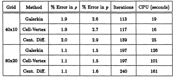
5.1 Exact Solution for 5* Channel Flow . ... . 65

5.2 Summary of Computed Solutions to 5* Wedge Problem . ... 66

5.3 Exact Solution for 15* Channel Flow . ... . 67

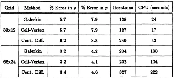
5.4 Summary of Computed Solutions to 15* Wedge Problem ... . 68

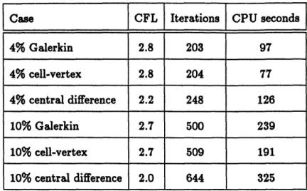
5.5 Comparison of Computational Effort for Circular Arc Bumps ... 71

5.6 Conservation in M, = 1.4, 4% Bump Case . . . . 72

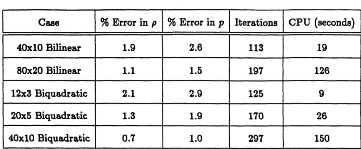
5.7 Comparison of Bilinear and Biquadratic Galerkin Solutions to 5* Wedge Problem ... 75

6.1 CPU Comparisons for Mo, = 1.4, 4% Bump . ... 117

6.2 CPU Comparisons for Mo, = 5 scramjet . ... 118

6.3 CPU Comparisons for Mo = 0.68, 10% Bump . ... 118

Chapter 1

Introduction

Computational methods are playing an ever-increasing role in the design of flight vehicles [25,62]. With the current computational power available, flow over (or in) realistic geometries can be calculated, if a computational grid can be generated. This need for geometric flexibility has given rise to unstructured grid algorithms, called finite element algorithms in this thesis. This thesis develops a new, adaptive finite element algorithm for the Euler equations describing the flow of an inviscid, compressible, ideal

gas.

1.1

Research Goals

The research presented here has four main goals. The first goal is the development of an adaptive finite element solution algorithm for the solution of the steady Euler equations in two and three dimensions using quadrilateral and hexahedral elements. To the author's knowledge, this thesis presents the first use of adaptation by grid embedding using hexahedral elements in three dimensions. Hexahedral elements offer large CPU and memory reductions over tetrahedral elements, and quadrilateral elements have a similar, although less marked, advantage in two dimensions. Significant computational cost reductions for a given level of accuracy are obtained with the adaptive algorithm. The new features here are the use of a multistage time integration scheme and the development of the adaptive hexahedral element in three dimensions.

The second goal is the development of a biquadratic finite element for the two-dimensional Euler equations. A single biquadratic element should be more accurate than the four bilinear elements it would replace on a grid with a comparable number of nodes. While quadratic elements have been tried before with only limited success [12], this thesis develops and demonstrates the utility of the higher-order elements, and presents results indicating increased accuracy at reduced computational cost.

The third goal is to compare several unstructured grid numerical methods, the Galerkin method, the cell-vertex method, and the central difference method, and to show the differences between them. This will (hopefully) end some of the current con-fusion in the literature by demonstrating that many of the currently used algorithms are finite element methods in disguise, and allow discussion to be focused on the issues of structured grid vs. unstructured grid and algorithm selection.

The fourth goal is the explanation of the low wave number numerical errors which occur near regions of high gradient in many problems. A dispersion analysis is presented which allows one to predict both the frequency of the oscillations and their location as a function of physical and computational parameters such as Mach number, grid aspect ratio and solution algorithm.

1.2

Overview of Thesis

The thesis begins with a brief survey of current research in finite element methods as applied to the Euler equations. Chapter 2 introduces the governing equations and the boundary conditions used in this thesis. Chapter 3 presents some fundamental concepts of finite element methods, and derives the bilinear, biquadratic, and trilinear elements. Chapter 4 presents a complete description of the solution algorithm, and demonstrates

that many other numerical methods can be cast into a finite element form. Chapter

5 presents some examples to verify the implementation of the numerical solver, and

presents a comparison of three particular computational methods often used to solve the Euler equations. Two of these methods are shown to be robust, efficient methods for the solution of the Euler equations. Chapter 6 introduces the idea of adaptation, and presents examples showing how it can reduce the computational cost for a given level of accuracy, and how adaptation can reduce the sensitivity of a solution to a poor initial grid. Chapter 7 presents a dispersion analysis of the numerical methods, and introduces the concept of spatial group velocity. The spatial group velocity can be used to predict the location of certain types of low wave-number solution errors. Chapter 8 returns to the physical world and examines some of the interesting features of flows in scramjet inlets. Chapter 9 draws some conclusions from this research and suggests areas for future exploration. The thesis is completed with an appendix illustrating some of the computational issues in finite element methods, followed by appendices containing the listings of the computer codes.

1.3

Survey of Finite Element Methods for the Euler

Equations

This section provides a brief review of the history of the finite element algorithm described in this thesis, and indicates other research going on in the field. The survey paper by Jameson [24] provides a good background for the history of numerical methods for the Euler equations. In 1954, Lax published a paper on the solution of hyperbolic equations with weak solutions [351. Several years were spent laying the mathematical foundations for the solution procedures, and in the late 1960's and early 1970's the first Euler solvers began to emerge [461. These early solvers were severely limited by

the computational power available in those days. As a result, much of the CFD effort was based on the solution of the transonic full potential equations. As the 70's turned into the 80's, computer capabilities increased enough to make the solution of the Euler equations practical. The finite volume methods of Jameson [281 and Ni [51] date from this time. About this time, it also became possible to compute the flow over realistic two-dimensional geometries, and unstructured grid ideas began to migrate from struc-tural mechanics into fluid mechanics. Much of the pioneering work on unstructured grids was done by French researchers at INRIA and Dassault [7]. In the mid 1980's, several unstructured algorithms began to emerge, and as newer computer architectures with larger memories and hardware scatter/gather became available, more researchers shifted into the unstructured mesh arena, some with "finite volume" methods, and others with "finite element" methods. At present, finite element methods are gaining widespread acceptance in fluid mechanics, and many researchers are investigating the use of unstructured grids for the solution of realistic problems.

There are many different formulations of the finite element method in the literature. Finite element algorithms different from the algorithm used in this thesis include the Petrov-Galerkin method (in which the test functions change with the solution to pro-duce an oscillation-free solution) [21], the Euler-Taylor-Galerkin method (essentially a Lax-Wendroff type method with a finite element spatial discretization) [6,13], Clebsch-transformed variables (corrections to the potential equations) [15] and various direct methods (Newton solvers) [8,18].

A sampling of other researchers in finite element methods includes Hughes, et al. at Stanford [22,20], Kennon [30] and Oden [52] at the University of Texas, LShner [43,40,391 at the Naval Research Lab, a group in Virginia at NASA Langley and Old Dominion University [6,58,71], Jameson from Princeton [27], a group at Swansea [48,53,54], groups

at INRIA and Dassault [3,55,671, and several groups in Japan [50,661. Although the term finite element is not used, the work of Dannenhoffer [9,11], can also be considered a finite element method. Many other groups throughout the world are also turning their attention to the development of unstructured grid methods for the Euler and Navier-Stokes equations [41]. The current interest in finite element and unstructured grid computational methods shows no signs of abating, and more researchers enter the field every year.

Chapter 2

Governing Equations

This chapter introduces the governing equations used throughout the remainder of the thesis. The non-dimensionalization of the equations is discussed, and the boundary conditions are described. Finally, some of the limitations of the equations are discussed.

2.1 Euler Equations

The equations solved are the Euler equations describing the flow of a compressible, inviscid, ideal gas. For these equations to hold, the following assumptions are necessary:

* The fluid is a homogeneous continuum; * The Reynolds number is infinite (inviscid); * The Peclet number is infinite (non-conducting); * The fluid obeys the ideal gas law.

While these assumptions do not hold exactly for any real flow, for a large class of problems they are a very good approximation. This thesis considers solutions to the steady-state Euler equations, but since the solution method involves a pseudo-time marching scheme the unsteady Euler equations are described here. Also, no body forces are considered in these equations.

The Euler equations in three dimensions can be written in conservation form as

p pu pV pw

pu pua + p put puw

a a a a

F pt +

pus

+

pv2 +p

+

p w

= 0,

(2.1)

pw puw pVw pW2 + p

pe puho pvho pwho

where where e is total energy, p is pressure, p is density, u, v, and w are the flow velocities in the z, y, and z directions, and ho is the total enthalpy, given by the thermodynamic relation

ho

=

e+ .

(2.2)

P

In addition, one requires an equation of state in order to complete the set of equations. For an ideal gas, this can be written

)

(7 e I- + , (2.3)

P 2

where the specific heat ratio y = 1.4 is constant for all calculations reported.

It is convenient to write the equations in vector form as

dU aF aG 8H

+ a +

+

+ --

= 0,

(2.4)

where U is the vector of state variables and F, G, and H are flux vectors in the x,

y, and z directions, corresponding to the vectors in Eq. (2.1) above. To restrict these

equations to two dimensions, drop the z derivatives and the z momentum equation.

The Euler equations described above provide a complete description of the com-pressible flow of an inviscid, non-conducting, ideal gas in the absence of body forces. For many problems this is a reasonable set of restrictions, but there are flows of interest where the Euler equations will not suffice. Each of the assumptions involved in the formation Euler equations will be examined.

The assumption that the fluid is continuous and homogeneous can break down for very low density flows, such as flow in the upper atmosphere or flows involving the mixing of multiple components. The assumption that the fluid is inviscid means that the Euler equations are inadequate if one is interested in viscous phenomena such as skin friction, boundary layers, separation and stall, or viscous-inviscid interaction. The non-conducting assumption means that heat transfer problems cannot be modeled. In many cases the ideal gas law breaks down. These can include problems in hypersonics in which the gas can dissociate and/or excite additional internal energy modes, combustion and other chemically reacting flows, and free-molecule flow (this also violates the first assumption). Finally, flows in which body forces are important (weather prediction or magnetohydrodynamics, for example) require the addition of additional terms to the equations.

2.2 Non-Dimensionalization of the Equations

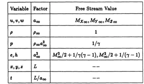
It is often convenient to non-dimensionalize the governing equations for a problem, since this clarifies the scales important to a problem, makes solutions independent of any particular system of units, and often helps reduce the sensitivity of a numerical solution to round-off errors. Table 2.2 lists the scaling factors for each of the problem variables. With this non-dimensionalization, the Euler equations become

p' p'· p'v' p'w'

p'u' p'u2 + p' p'lu'' p'I'w'

a9

a

a

a

Ft

p''

+

p'u'v'

+

4

'u

+p'

az

p'v'w'

=

(2.5)

p'w' p'u 'w' P'V'w' pw'2 + p'

p'e' p'u'hg p','h6 p'w'hg

where the ' variables are non-dimensional. This non-dimensionalization shows that the Euler equations have two associated non-dimensional parameters, which enter through

Table 2.1: Scaling Factors for Non-Dimensionalization

the boundary conditions and the state equation: the Mach number M and the ratio of specific heats y. Note that the non-dimensional parameters associated with the Euler equations do not appear in Eq. (2.5). Since this is the case, all further discussions will be based on the non-dimensional variables, and the ' superscript will be dropped.

2.3

Auxiliary Quantities

It is convenient to define a number of auxiliary physical quantities in terms of the primitive quantities p, u, v, w, and p. These are the following:

Local speed of sound:

Mach Number:

Total Pressure:

Total Pressure Loss:

Entropy:

a

Ploss = Po-P

Poo-AS = log _pr

Variable Factor Free Stream Value , v, aoo M 0 0, My 00, Mz 0 0 P Poo 1 2 l/y P PoaO 1/ e, h a~ M2/2 + 1/7(1 - 1), M2/2 + 1/(y - 1)

z, y, z

L

--where the free stream entropy is defined to be 0.

2.4

Boundary Conditions

In order to solve any set of differential equations, boundary conditions need to be specified. In this thesis, two types of boundaries are defined for the Euler equations: solid surfaces and "open" boundaries. The implementation of these boundary conditions is discussed in Section 4.4.

2.4.1

Solid Surface Boundary Conditions

At a solid surface boundary, there is no mass flux normal to the boundary. This is equivalent to saying

u,* A = 0,

(2.6)

where & is the velocity vector and A is the unit normal to the surface.

2.4.2

Open Boundary Conditions

The "open" or far-field boundary conditions are based on quasi-one-dimensional

boundaries are neglected. The resulting equations are diagonalized assuming locally

isentropic flow, yielding the characteristic equations

a

+

_{(u + a)}

_{= 0,}

_(2.7)

BR

+ (aR - a)

aR

_0,

(2.8)

aut

au

u

+

u

-

=

0,

(2.10)

as

as

-

+ U

_{= 0,}

_(2.11)

where (t, rl, •) are the transformed directions, with C normal to the boundary, S is the entropy, u, and ut are the velocities tangential to the boundary, and Q and R are the Riemann invariants [36]

2a

Q

R = u - _- , (2.13)

-1

derived from the diagonalized system. If there is no entropy variation normal to the boundary, these invariants are exact, otherwise they are approximate. These equations are decoupled wave equations, and so these characteristic variables are convected normal to the boundary in a direction determined by the sign of the associated wave velocity. For example, if 0 < uE < a, the boundary is a subsonic inflow boundary, so

Q,

Chapter 3

Finite Element Fundamentals

This chapter introduces some of the important concepts in finite element methods. The terms element, node, edge and face are defined, and the transformations between physical and computational space are described. A discussion of derivative calculation is given, and the 4-node, 2-D bilinear, the 9-node, 2-D biquadratic, and the 8-node, 3-D

trilinear elements are developed.

3.1

Basic Definitions

The finite element method subdivides the physical domain of interest into small subdomains called elements, each of which is composed of some number of nodes. Fig-ure 3.1 shows how a domain might be divided into elements, in this case six. The nodes are indicated by the black circles. Note that not all the elements are made up of the same numbers of nodes. For example, the mesh shown has pentagonal, quadrilateral and triangular elements. The finite element method does not restrict one to identical elements, in general. Quadrilateral and triangular elements in two dimensions have been combined in a single problem, by Ramakrishnan, for example [58]. In actual practice one usually only uses a few different types of elements in a particular problem. For a real problem, a domain will typically be divided into hundreds, thousands, or hundreds of thousands of elements.

6 Elements, 10 Nodes

Figure 3.1: Example of a General Finite Element Discretization

element dimension and composed of element intersections. An edge is the intersection of faces. Note that in two dimensions, an edge and a node are the same thing, but in three dimensions they are not. Figure 3.2 shows faces and edges in two and three dimensions.

In this thesis, quadrilateral elements are used in two dimensions and hexahedral elements are used in three dimensions. The algorithm itself is applicable to arbitrary polygons and polyhedra. The advantage of quadrilateral and hexahedral elements is that for a given number of nodes, a triangular mesh will have roughly twice as many elements as a quadrilateral mesh, and in three dimensions, a tetrahedral mesh will have roughly five times as many elements as a hexahedral mesh. Since there are many operations that are performed on elements, there is a significant potential for memory and CPU savings with reduced numbers of elements. The disadvantages of the quadrilateral and hexahedral elements are that grid generation may be more difficult for some problems, and where grid embedding is used, there is the problem of interface treatment. On the other hand, the formulation of the finite element method permits the use of degenerate

Face

Edge

Node

2-D 3-D

Figure 3.2: Definition of Finite Element Terms

3

2

1

Node Numbering: 1-2-3-1

Figure 3.3: Quadrilateral Element Degenerated into a Triangular Element elements, that is, elements in which one or more nodes are repeated to form an element with a smaller effective number of nodes. Figure 3.3 shows how a quadrilateral element can be degenerated into a triangular element by repeating node 1, for example. At this point it is important to emphasize the unstructured nature of the finite element method. In the finite element method, all operations are done at the element level, with element contributions assembled (distributed) to the nodes. Computationally, there are no structures such as grid lines, although one may see something that looks like a grid line in a picture of a mesh. This distinction is what give finite element methods their

flexibility. It is not necessary for each grid point to be indexed by (i, j, k) or by some similar scheme, and a node may belong to any number of elements.

A vast literature exists describing finite element, finite volume and finite difference

algorithms for various equations. As will be shown in Section 4.3, many of the finite volume and finite difference algorithms can be viewed as finite element algorithms, so the real distinction should not be one of name (finite element, volume or difference) but of substance (structured mesh or unstructured mesh, what the difference stencil actually looks like, etc.)

3.2

Finite Elements and Natural Coordinates

The finite element method provides a way to make a convenient transformation be-tween a local, computational space (natural coordinates) and a global, physical space. The following discussion will emphasize this in two dimensions, but the ideas are iden-tical in three dimensions (or even in one dimension).

In the finite element discretization one assumes that within each element, some quantity q(e) is determined by its nodal values qi and a set of shape or interpolation functions Nie) so that

q(e) - N(e)qi, (3.1)

i=1

where m is the number of nodes in the element. The elemental shape functions are summed to give global shape functions Ni, so that globally q can be written

M

q(z, y) = (N-(, y) q, (3.2)

i= 1

3.2.1

Properties of Interpolation Functions

The interpolation functions NMe) (also called shape functions or trial functions) must have certain properties in order for the finite element approximation to be valid. These properties are as follows:

1. The shape function N"() must be 1 at node i and 0 at all other nodes of the domain. This is required so that the relation in Eq. (3.2) can hold for each node. 2. The shape function NMe) should be 0 outside of element e. Strictly speaking, this is only required if one desires a local finite element approximation. All the shape functions used in this report are local and satisfy this property. A consequence of this property is that the global shape function Ni at node i is just a union of the elemental shape functions N( e) for all the elements containing node i.

3. In each element, the sum of all the nodal shape functions Ni() should be identically

1. This is so the constant function can be represented exactly (a requirement for

consistency in the approximation).

There are two things to note about these requirements. First, requirements 2 and

3 imply that constant functions can be represented exactly for all geometries. Second,

these requirements do not force the shape functions to be continuous between the el-ements, and some researchers have made use of discontinuous trial functions in their formulations [2,30]. In this report, all interpolation functions will be continuous in the elements and across the element boundaries.

Typically, interpolation functions are chosen to be polynomials in some natural co-ordinates (;, r). The degree of the polynomial approximation is related to the accuracy

has found that for many structural mechanics problems, biquadratic interpolation

func-tions give better results than bilinear interpolation funcfunc-tions [65], but in the solution of

the Euler equations the question of the optimal order of shape function is still an open

one.

3.2.2 Natural Coordinates and Derivative Calculation

Interpolation functions are usually chosen to be polynomials in some natural coor-dinate system (e, r/). Strang [69] indicates that polynomials are the optimal choice for interpolation functions in the sense that in order to obtain an kth order accurate ap-proximation to an sth derivative on a regular mesh, the interpolation functions must be complete (be able to represent exactly) all polynomials of degree k + 8 - 1. Thus, a set

of polynomials will have the smallest number of elements for a given order of accuracy. The geometry of the element is interpolated in terms of nodal coordinates. That is, one states that within an element,

y(e) = NP')(e,9i)yi, (3.4)

where xz and yi are the coordinates of node i in element e. For simplicity, all derivations are shown in two dimensions, and the extension to three dimensions is straightforward.

It is useful to be able to write the derivative of a quantity in terms of the nodal values of that quantity. Since the derivatives are usually desired in physical space, we require the Jacobian of the transformation. One can write:

1

a

:

=

J

18

(3.5)

where J is the Jacobian matrix (valid within each element)

Sax

ay

1aN

e)

8N

()

J= a

at

at

at

(3.6)

ax

ay

8Nr

e)

aN8

When J is known (and non-singular), J-1 can be calculated, so one can write the derivatives of a quantity q in each element as follows:

ax

=J

-1 "

a

_(3.7)

Oq 8 N.(e)

where the q, are the nodal values of q. Note that this requires the Jacobian to be non-singular for all e and 'i in the element. For the bilinear transformation, this will be true if, and only if, the element is convex in physical coordinates. To see this, note that

jJj

j

IJI

IJI

If the same shape functions are used to interpolate both the element geometry and the quantity q, the element is called an isoparametric element. If the shape functions used to interpolate the geometry are of a lesser degree than the interpolation functions for the quantity q, the element is termed subparametric. In this thesis, isoparametric bi- and trilinear elements and subparametric biquadratic elements are used.

3.3

Typical Elements

Figure 3.4 shows the geometry for the 4-node bilinear and 9-node biquadratic ele-ments in both physical and natural coordinates. This figure also shows the node and

.'I ,1 -1,1 ) (-1,-1) 4 3 2 (1,1) I-(1,-1)

Physical Coordinates Natural Coordinates

Node numbering in bold, face numbering in italic Figure 3.4: Geometry of Two-Dimensional Element

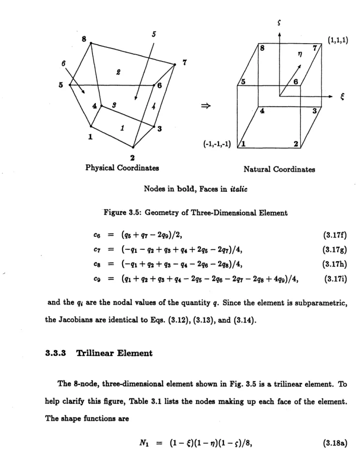
face numberings used at the element level. The open circles indicate nodes that are present only in the 9-node element. Figure 3.5 (on page 38) shows the equivalent infor-mation for the three-dimensional, trilinear element. To help clarify this figure, Table 3.1 lists the nodes making up each face of the element.

3.3.1 Bilinear Element

The section presents the shape functions for the bilinear, 4-node element and gives the explicit formulas for the Jacobian and its inverse. See Fig. 3.4 for the geometry of the element. In natural coordinates, the nodal shape functions are

Ni = (1 - C)(1 - rq)/4, (3.8a)

N2 = (1 + C)(1 - 7)/4, (3.8b)

Ns = (1+ C)(1 + l)/4, (3.8c)

N4 = (1 - C)(1 + q)/4, (3.8d)

and one can write 4

X(C, ) =

7),

(xiNi(,

(3.9a)

y(,j ) =

yiN(~(, •),

(3.9b)

q (, t) =

q Ni,

(,7),

1

(3.9c)

where zx and yi are the coordinates of the nodes and qi are the nodal values of some quantity q. It will be convenient to expand these quantities:

z(C,r)

=

aj

+

a2C+a

•

cs,

+

a

(3.10a)

y(e,r9)

=

b + b

+ b

t + bs

&,

(3.10b)

q(C,t1)

= c1

+

c

2+

cs

+

c

,

(3.10c)

where the coefficients al, a2, as, as are

al = ( z1 + z2

+

a2 = (-z+Z2 z3 - 4)/4, (3.11b)

as = (-X1 - X2 + Xs + z4)/4, (3.11c)

as = ( zl - z 2 + z3 -- 4)/4, (3.11d)

and similarly for b and c. The er term has the subscript "5" instead of the subscript "4" to reserve the subscript "4" for the C2 term in the biquadratic expansions following.

Now the Jacobian can be formed. Writing in terms of the a's and b's,

a2 + a5r b2

+

_(3.12)

as + as5

b

+ bs

1

bs

bsbs+ -(b + b)

(3.14)

-(as

+

as)C a2 + asr

so derivatives (and integrals) of quantities can now be calculated in physical coordinates.

3.3.2 Biquadratic Element

The biquadratic element used is a subparametric, 9-node element. The geometry is interpolated exactly as the bilinear element just described. This section presents the analogs to Eqs. (3.8) and (3.11). The biquadratic shape functions are

N

t)/2,

N

q

+

N

so that one can write some quantity q as

q = cl + C2C -+ cr + c4( 2 + C5 Cs + c t2 + c-7t 2

r+

t1

(3.16).

+

t

8

7

17

1 2

Physical Coordinates _{Natural Coordinates}

Nodes in bold, Faces in italic

Figure 3.5: Geometry of Three-Dimensional Element

= (qs + q7 - 2q9)/2,

= (-ql -

q2

+ qa +

q4

+ 2qs - 2q

7

)/4,

= (-ql +

q2

+ q3 - q4 - 2qe - 2q

8

)/4,

+

3.3.3 Trilinear Element

The 8-node, three-dimensional element shown in Fig. 3.5 is a trilinear element. To help clarify this figure, Table 3.1 lists the nodes making up each face of the element. The shape functions are

(3.18a) (3.18b)

(1,1,1)

V

1

₃₁

Table 3.1: Nodes for Each Face, Trilinear Element

Ns = (1+ )(1+r1)(1-

)/8,

N

(1=

+ )(1- t)(1+ -)/8,

0)(1

and one can write

q = d, + d2C + dsi7 + d4ý + ds,5e + d6plg + d7Cg + dse%),

where ( ql + q2 + q3 + q4 + q5 (-ql + q2 + q3 - q4 -qs (-ql - q2 + q0 + q4 - qs (-qi - q2 - q3 - q4 + q5 ( ql-q2+q3-q4+-q5 ( q+ q2 - q3-q4 - qs

(

ql-q2-qs+q4-qs

+ q6 + q+

- q8)/8,

-

q6

+ q7 +

q8)/8,

+

6

+ q7 - q8)/8,

- q6 + q7 +

q8)/8,

q7

+ q6 + q7 - q8)/8,

The Jacobians are calculated in a similar manner as those above. Due to the complex-ity of the expressions involved, only the Jacobian matrix itself is shown. The

three-Face Nodes on three-Face three-Face Nodes on three-Face

1 1-2-3-4 4 2-3-7-6 2 5-6-7-8 5 4-3-7-8 3 1-2-6-5 6 1-4-8-5 (3.18c) (3.18d) (3.18e)

(3.18f)

(3.20b)

dimensional Jacobian J is

a2 + asr + a7ý + a b b2+b

+

+

+

S= a+ as + a

+ a

88

+

,

+b

(3.21) where ai, bi, and ci are the coefficients in the expansions of x, y, and z in the element.

Chapter 4

Solution Algorithm

This chapter describes in detail the finite element solution algorithm for the Euler equations. The application of the finite element method to the spatial discretization is described, and section 4.3 introduces the Galerkin finite element, "cell-vertex" finite element and "central difference" finite element methods. The implementation of bound-ary conditions is discussed in section 4.4. All of these methods require added damping for stability, and this is discussed in section 4.5. Section 4.6 describes the pseudo-time marching method. Finally, section 4.7 describes the conditions on the test and trial functions needed to obtain consistency and conservation.

4.1

Overview of Algorithm

This section describes briefly the steps taken in the solution of a problem; each step is discussed in detail in the following sections. The steady-state Euler equations are solved using a pseudo-time marching technique. This means that from some initial condition, the solution is evolved by an iterative technique resembling the solution of the unsteady problem until it stops changing. This time marching consists of three steps. First, a residual representative of the difference between the steady solution and the current solution is calculated. Second some additional damping terms are added to this residual. Third, the current solution is updated to obtain the next approximation. This process is repeated until the desired degree of convergence is obtained. Convergence is

signaled when the RMS of all changes divided by the RMS of all the state vectors is less than some specified number, usually around 10- 5. Other norms are possible, but

the differences in the solutions produced by different indicators are not significant.

A new contribution is the use of the four-step multistage time integration scheme.

Previous work has often used a two-step Lax-Wendroff time integration method [6,43], but Ramakrishnan, Bey and Thornton have shown that the multistage time integration method developed herein has better stability properties than the two-step Lax-Wendroff time integration method when used with adaptive meshes [58].

4.2

Spatial Discretization

The spatial discretization method begins with the Euler equations in conservation law form ( Eq. (2.4) ) written

aU

8F

8H

+ + + -- = 0, (4.1)

at at By 8z

where U is the vector of state variables and F, G, and H are flux vectors in the z, y, and z directions. Within each element the state vector U(e) and flux vectors F(e), G(e)

and H(C) are written

U( ) = - Z N(e)U-, (4.2)

F(C) = EN()Fi,

(4.3)

G(C) = EN(')G-,

(4.4)

H(e)

=

E

N(')Hý,

(4.5)

where Ui, F,, GC and H% are the nodal values of the state vector and flux vectors, and NS( ) is the set of interpolation functions for element e.