Accelerated parallel magnetic resonance imaging
reconstruction using joint estimation with a sparse signal model
The MIT Faculty has made this article openly available.
Please share
how this access benefits you. Your story matters.
Citation
Weller, Daniel S., Jonathan R. Polimeni, Leo Grady, Lawrence L.
Wald, Elfar Adalsteinsson, and Vivek K Goyal. “Accelerated Parallel
Magnetic Resonance Imaging Reconstruction Using Joint Estimation
with a Sparse Signal Model.” 2012 IEEE Statistical Signal Processing
Workshop (SSP) (n.d.).
As Published
http://dx.doi.org/10.1109/SSP.2012.6319666
Publisher
Institute of Electrical and Electronics Engineers (IEEE)
Version
Author's final manuscript
Citable link
http://hdl.handle.net/1721.1/85876
Terms of Use
Creative Commons Attribution-Noncommercial-Share Alike
ACCELERATED PARALLEL MAGNETIC RESONANCE IMAGING RECONSTRUCTION
USING JOINT ESTIMATION WITH A SPARSE SIGNAL MODEL
Daniel S. Weller
1, Jonathan R. Polimeni
2,3, Leo Grady
4,
Lawrence L. Wald
2,3, Elfar Adalsteinsson
1, Vivek K Goyal
11
Dept. of EECS, Massachusetts Institute of Technology, Cambridge, MA, USA
2
A. A. Martinos Center, Dept. of Radiology, Massachusetts General Hospital, Charlestown, MA, USA
3Dept. of Radiology, Harvard Medical School, Boston, MA, USA
4
Dept. of Image Analytics and Informatics, Siemens Corporate Research, Princeton, NJ, USA
dweller@mit.edu, jonp@nmr.mgh.harvard.edu, leo.grady@siemens.com,
wald@nmr.mgh.harvard.edu, elfar@mit.edu, vgoyal@mit.edu
ABSTRACT
Accelerating magnetic resonance imaging (MRI) by re-ducing the number of acquired k-space scan lines benefits conventional MR imaging significantly by decreasing the time subjects remain in the magnet. In this paper, we formu-late a novel method for Joint estimation from Undersampled LinEs in Parallel MRI (JULEP) that simultaneously calibrates the GeneRalized Autocalibrating Partially Parallel Acquisi-tions (GRAPPA) reconstruction kernel and reconstructs the full multi-channel k-space. We employ a joint sparsity signal model for the channel images in conjunction with observation models for both the acquired data and GRAPPA reconstructed k-space. We demonstrate using real MRI data that JULEP outperforms conventional GRAPPA reconstruction at high levels of undersampling, increasing peak-signal-to-noise ra-tio by up to 10 dB.
Index Terms— Magnetic resonance imaging, image re-construction, parallel imaging, sparsity, Bayesian estimation
1. INTRODUCTION
In conventional magnetic resonance imaging (MRI), the de-sired image or volume commonly is acquired by raster scan-ning the spatial Fourier transform domain called k-space, sampling these scan lines, and taking the inverse Fourier transform of these samples. MR imaging is fundamentally limited by the time required to trace all these scan lines. Greatly accelerating MRI by reducing the number of lines acquired is accompanied by reductions in image quality. Ac-celerated parallel MRI undersamples k-space, using fewer lines spaced farther apart, reducing the field of view (FOV), and introducing aliasing when the object is larger than the
Funding acknowledgments: NSF CAREER Grant CCF-0643836, NIH R01 EB007942 and EB006847, NIH NCRR P41 RR014075, Siemens Cor-porate Research, and an NSF Graduate Research Fellowship.
reduced FOV; parallel imaging resolves this aliasing and produces a full-FOV image using parallel receivers.
Compressed sensing (CS) leverages the compressibility of MR images to reconstruct images from randomly under-sampled data [1]. Methods like SENSE [2], GRAPPA [3], and SPIRiT [4] also are effective for reconstructing images from undersampled data, but these methods are affected by noise amplification or residual aliasing at high levels of ac-celeration. The synergistic combination of SENSE [5] or SPIRiT [6] with CS aims to address the shortcomings of ac-celerated parallel imaging and achieve acceleration beyond what is achievable with either approach individually.
The synergistic combination of GRAPPA with a spar-sity model is more complicated due to characteristics of GRAPPA including the presence of a calibration step, the use of uniformly-spaced (nonrandom) undersampling, and the reconstruction of multiple channel images rather than a single combined image. Building upon the previous develop-ment of sparsity-based DESIGN denoising [7] of GRAPPA-reconstructed data and sparsity-promoting GRAPPA kernel calibration [8], we reinterpret the sparse reconstruction prob-lem and devise a method for Joint estimation from Undersam-pled LinEs in Parallel MRI (JULEP) that elegantly unifies the kernel calibration and full k-space reconstruction/denoising problems with a single solution. This proposed method im-proves reconstruction quality at high levels of acceleration, accommodating both greater spacing between k-space sam-ples and fewer autocalibration (ACS) lines.
2. THEORY
Consider the N × P matrix Y, whose columns represent the full k-space we wish to estimate for each of the P coil chan-nels. Each of the coil images is presumed to be approximately sparse in some appropriate transform domain with analysis
(forward) transform Ψ. Let W = ΨF−1Y, where F is the discrete Fourier transform; then we can impose a sparsity model on W corresponding to the `p,qmixed norm,
parame-terized by λ > 0, which controls the level of sparsity:
p(W) ∝ e−λkWkpp,q =
N −1
Y
n=0
e−λk[W1[n],...,WP[n]]kpq. (1)
To maintain convexity, we choose p = 1 (one could also im-pose priors for 12 < p < 1; see [9]). Setting q = 1 favors channel-by-channel sparsity, where the support of each trans-formed channel image is considered independently of those of the other channel images. For joint sparsity [10], where the supports of each transformed channel are assumed to over-lap sufficiently to gain by assuming all the channels share the same support, we can set q = 2 (loose joint sparsity) or q = ∞ (strict joint sparsity) to tie these channels together. In this work, we proceed assuming loose joint sparsity and set q = 2. Assuming W is complex, p(W) = N −1 Y n=0 P !λ2P (2P )!πPe −λk[W1[n],...,WP[n]]k2. (2)
In accelerated MRI, the full k-space can be subdivided into Ya = KaY, the acquired k-space, and Yna = KnaY,
the un-acquired k-space. From the acquisition, we have direct observations of acquired k-space Da, and based on the large
number of individual spins, we model our observation noise as complex Gaussian (with real and imaginary parts uncorre-lated). As the noise is typically assumed to be random pertur-bations due to thermal and other uncorrelated variations, we assume this noise is iid across k-space frequency measure-ments, and we allow for correlation across channels for the same frequencies. Formally,
p(Da| Y) = CN (vec(Da); vec(KaY), IM ×M⊗ Λ), (3)
where CN (·; µ, Λ) is the density function of the complex Normal distribution with mean µ and covariance Λ, vec(·) stacks the columns of a matrix into one vector, and ⊗ is the Kronecker product.
Additionally, the GRAPPA reconstruction method pro-vides observations of the un-acquired data. Given the ap-propriate GRAPPA kernel G, the GRAPPA reconstruction ideally yields Yna= GRAPPA(G, Ya). Since GRAPPA is
linear in Ya, substituting Dayields Yna+ amplified noise.
Calling these GRAPPA-reconstructed observations Dna, the
likelihood of Dnagiven the full k-space Y is
p(Dna| Y) = CN (vec(Dna); vec(KnaY), ΛG), (4)
where the amplified noise has covariance ΛG.
Putting these signal and observation models together, the minimum mean squared error estimator is the posterior mean E{Y | Da, Dna}. Due to variable mixing in both the
sig-nal and observation models, this estimator does not have a
closed form, and numeric integration methods like quadra-ture are computationally infeasible (due to the curse of di-mensionality). One could resort to stochastic methods (e.g. importance sampling), but convergence may be rather slow due to the number of correlated variables involved. Instead, we propose finding the maximum a posteriori (MAP) esti-mate, a compressed sensing-like optimization problem:
Y = minimize Y 1 2k vec(KaY − Da)k 2 IM ×M⊗Λ+ 1 2k vec(KnaY − Dna)k 2 ΛG+ λkΨF −1Yk 1,2. (5)
The notation kxkΛ is shorthand for kΛ−1/2xk2(for
Hermi-tian symmetric positive definite Λ). This simple estimator can be implemented and solved using various techniques, includ-ing iteratively reweighted least squares (IRLS) [11]. The use of IRLS to solve this type of problem is carefully illustrated in [7, 8]. This formulation effectively denoises the acquired and GRAPPA reconstructed k-space, similar to the DESIGN denoising method already developed.
Now, suppose the GRAPPA kernel G is now an unknown variable, instead of simply being computed from the ACS lines. From the matrices of source points Ysand target points
Ytfrom our ACS lines, with observations Dsand Dt, we add
observations of the form GDs= Yt+ noise. Assuming that
the source points follow the same observation model as the other acquired data, the noise will be complex Gaussian and amplified by the GRAPPA kernel (call the noise covariance ΛACS). The optimization problem now becomes joint over
the full k-space Y and the GRAPPA kernel G: {Y, G} = minimize Y,G 1 2k vec(Yt− GDs)k 2 ΛACS+ 1 2k vec(KnaY − GRAPPA(G, Da))k 2 ΛG+ 1 2k vec(KaY − Da)k 2 IM ×M⊗Λ+ λkΨF −1Yk 1,2. (6)
At first glance, this optimization problem has the same form as Eq. (5); however, the covariance matrices ΛG and
ΛACSdepend on G, so the first two parts of the objective are
not strictly least-squares terms, and the overall problem is not convex. We approach the problem by fixing these covariance matrices, applying IRLS to form an iterative algorithm, and update the covariance matrices at the same time we update the diagonal IRLS re-weighting matrix ∆.
{Y, G} = minimize Y,G 1 2k vec(Yt− GDs)k 2 ΛACS+ 1 2k vec(KnaY − GRAPPA(G, Da))k 2 ΛG+ 1 2k vec(KaY − Da)k 2 IM ×M⊗Λ+ λ 2k∆ 1 2ΨF−1Yk2 F, (7) where ∆n,n = k[W 1 1[n],...,WP[n],ε]k2, with W = ΨF −1Y
log |k-space| F−1 −−−→ image Ψ −→ DWT
Fig. 1. This T1-weighted image, acquired in the k-space
do-main, has a sparse four-level ‘9-7’ DWT representation.
Since Eq. (6) is not convex, convergence to a global minimum is not guaranteed, and initialization affects the solution. The initial full k-space is zero-filled, containing only the acquired data, and the initial GRAPPA kernel is the least-squares or minimum energy solution to the system of ACS fit equations (G = DtD†s, where D†sis the left or right
pseudo-inverse of Ds). We anticipate convergence when
the objective decreases by less than tol percent. While this criterion is susceptible to the possibility that updating ΛACS
and ΛG can increase the objective, such behavior did not
hamper our simulations. Although the covariance matrices have lots of nonzero cross terms, because the GRAPPA ker-nel introduces correlations among k-space frequencies, we focus on the noise amplification aspect of GRAPPA by using a block diagonal matrix with correlations only across chan-nels (blocks are P × P ). The JULEP method is summarized below:
1. Set G and Y, and initialize ΛGand ΛACS.
2. Compute re-weighting matrix ∆ for the `1,2term using
the current estimate of Y.
3. Update G and Y using an iterative solver for Eq. (7). 4. Update ΛGand ΛACSbased on the new value of G.
5. Repeat steps (2)–(4) until the objective decreases by less than tol percent.
3. METHODS
A T1-weighted full-FOV image (256 × 256 × 176 mm FOV;
1.0 mm isotropic resolution) is acquired on a Siemens 3 T scanner using a Siemens 32-channel receive array head coil. An axial slice is extracted, cropped, and normalized; the com-bined magnitude reference image and its k-space are shown in Fig. 1 along with its sparse transform using a four-level ‘9-7’ 2-D DWT. The k-space is undersampled in both directions in the axial plane, a 36 × 36 ACS block is retained in the cen-ter of k-space, and full-FOV images are reconstructed using GRAPPA and the proposed method.
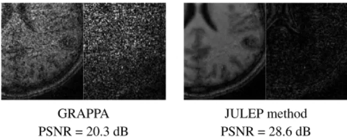
GRAPPA JULEP method
PSNR = 20.3 dB PSNR = 28.6 dB
Fig. 2. The inset images and difference images above sug-gest that while the GRAPPA reconstruction is very noisy, the JULEP joint estimated image has much less noise.
The channel noise covariance matrix Λ is measured from a separate noise-only (no RF excitation) acquisition. The re-constructed full k-space is combined to form a single com-bined magnitude image using the SNR-optimal coil combina-tion based on sensitivities estimated from apodized ACS lines and Λ. The magnitude images are compared using differ-ence images and peak-signal-to-noise ratio (PSNR). Although PSNR, as a non-specific measure, does not accurately reflect image quality as perceived by a clinician, it facilitates study of quantitative trends in image quality. A convergence threshold of tol = 1% is used for all experiments.
4. RESULTS
In the first experiment, the T1-weighted k-space shown in
Fig. 1 is nominally undersampled by a factor of 5 along the coronal axis (vertical direction) and a factor of 4 along the sagittal axis (horizontal direction), and a 36×36 block of ACS data is retained, for an effective acceleration of R = 12.1. For both the GRAPPA and JULEP algorithms, a GRAPPA kernel for 5 × 4 source points is calibrated for each of the target points. In the case of un-regularized GRAPPA kernel cali-bration, the calibrated kernel yields a GRAPPA-reconstructed image with significant noise amplification in about 1 second. The joint estimation of the kernel and full k-space produces a reconstruction in under 80 minutes (4 IRLS steps with a total of 555 inner iterations of the least-squares solver LSMR [12]) with far less noise than before while retaining important struc-tural information. The inset region (outlined by the rectangle in Fig. 1) of the reconstructed images alongside correspond-ing inset regions of the difference images in Fig. 2 portray a significant difference in image quality.
This experiment is repeated on the same image for both 4×4 and 5×4 nominal undersampling, changing the effective acceleration by varying the number of ACS lines, and com-paring the magnitude image PSNRs for both GRAPPA and joint estimation reconstructions. The trend lines portrayed in Fig. 3 confirm that as the effective acceleration increases due to having fewer ACS lines, the JULEP method consis-tently produces significantly higher quality images (as mea-sured crudely by PSNR). The ACS block grows from 35 × 35
8.5 9 9.5 10 10.5 15 20 25 30 Effective Acceleration (R) PSNR (dB) GRAPPA Joint estimation
(a) 4 × 4 nominal undersampling
9.5 10 10.5 10 15 20 25 30 Effective Acceleration (R) PSNR (dB) GRAPPA Joint estimation (b) 5 × 4 nominal undersampling
Fig. 3. As the number of ACS lines varies, changing the total acceleration, the JULEP joint estimation method consistently outperforms the GRAPPA reconstruction in terms of PSNR.
to 48 × 48 for the 4 × 4 nominally undersampled data, and from 42 × 42 to 48 × 48 for the 5 × 4 undersampled data. For fewer ACS lines, the number of fit equations is insufficient to perform a least-squares fit for the GRAPPA kernel calibra-tion. Similar improvement in image quality is observed in the first experiment, which uses underdetermined calibration.
5. DISCUSSION
The significant improvement in image quality achievable by the proposed JULEP joint estimation algorithm is evi-dent in both experiments, yielding 5-10 dB improvement over GRAPPA. When considering the number of ACS lines needed for a given nominal undersampling factor to achieve a minimum PSNR, this novel estimation method can achieve that PSNR with far fewer ACS lines. Shifting this trade-off has implications for MRI acquisitions where maximum ac-celeration is desired; i.e. ACS lines are expensive. While we cannot validate these methods clinically without extensive evaluation of images featuring abnormalities like lesions, the proposed method enables greater acceleration of MRI.
6. REFERENCES
[1] M. Lustig, D. Donoho, and J. M. Pauly, “Sparse MRI: The application of compressed sensing for rapid MR
imaging,” Magn. Reson. Med., vol. 58, no. 6, pp. 1182– 95, Dec. 2007.
[2] K. P. Pruessmann, M. Weiger, M. B. Scheidegger, and P. Boesiger, “SENSE: sensitivity encoding for fast MRI,” Magn. Reson. Med., vol. 42, no. 5, pp. 952–62, Nov. 1999.
[3] M. A. Griswold, P. M. Jakob, R. M. Heidemann, M. Nit-tka, V. Jellus, J. Wang, B. Kiefer, and A. Haase, “Gen-eralized autocalibrating partially parallel acquisitions (GRAPPA),” Magn. Reson. Med., vol. 47, no. 6, pp. 1202–10, June 2002.
[4] M. Lustig and J. M. Pauly, “SPIRiT: Iterative self-consistent parallel imaging reconstruction from arbi-trary k-space,” Magn. Reson. Med., vol. 64, no. 2, pp. 457–471, Aug. 2010.
[5] D. Liang, B. Liu, J. Wang, and L. Ying, “Accelerat-ing SENSE us“Accelerat-ing compressed sens“Accelerat-ing,” Magn. Reson. Med., vol. 62, no. 6, pp. 1574–1584, Dec. 2009. [6] M. Lustig, M. Alley, S. Vasanawala, D. L. Donoho,
and J. M. Pauly, “L1 SPIR-iT: Autocalibrating
paral-lel imaging compressed sensing,” in Proc. ISMRM 17th Scientific Meeting, Apr. 2009, p. 379.
[7] D. S. Weller, J. R. Polimeni, L. Grady, L. L. Wald, E. Adalsteinsson, and V. K Goyal, “Denoising sparse images from GRAPPA using the nullspace method (DE-SIGN),” Magn. Reson. Med., to appear.
[8] D. S. Weller, J. R. Polimeni, L. Grady, L. L. Wald, E. Adalsteinsson, and V. K Goyal, “Regularizing grappa using simultaneous sparsity to recover de-noised im-ages,” in Proc. SPIE Wavelets and Sparsity XIV, Aug. 2011, vol. 8138, pp. 81381M–1–9.
[9] D. S. Weller, J. R. Polimeni, L. Grady, L. L. Wald, E. Adalsteinsson, and V. K Goyal, “Evaluating sparsity penalty functions for combined compressed sensing and parallel MRI,” in Proc. IEEE Int. Symp. on Biomedical Imaging, March–April 2011, pp. 1589–92.
[10] S.F. Cotter, B.D. Rao, K. Engan, and K. Kreutz-Delgado, “Sparse solutions to linear inverse problems with multiple measurement vectors,” IEEE Trans. Sig-nal Process., vol. 53, no. 7, pp. 2477–88, July 2005. [11] P. W. Holland and R. E. Welsch, “Robust regression
using iteratively re-weighted least-squares,” Commun. Statist. A: Theory Meth., vol. 6, no. 9, pp. 813–827, 1977.
[12] D. C.-L. Fong and M. A. Saunders, “LSMR: An iterative algorithm for sparse least-squares problems,” SIAM J. Sci. Comput., vol. 33, no. 5, pp. 2950–2971, 2011.