Advances in component-based face detection

I

Advances in Component-based Face Detection

by

Stanley Michael Bileschi

Submitted to the Department of Electrical Engineering and Computer

Science

in partial fulfillment of the requirements for the degree of

Master of Science

at the

MASSACHUSETTS INSTITUTE OF TECHNOLOGY

January

2003-@

Massachusetts,,-stitute of Technology 2003. All rights reserved.

A uthor . ...

Depart nIt of Electrical Engineering and Computer Science

September 30, 2002

Certified

by.

...

.~

..

..

....

. ... ... ..

Tomaso Poggio

Uncas and Helen Whitaker Professor of Brain and Cognitive Sciences

Thesis Supervisor

Accepted by ...

...

...

Arthur C. Smith

Chairman, Departmental Committee on Graduate Students

MASSACHUSETS _{OF TECHNOLOGY}INSTITUTE

BARKER

Advances in Component-based Face Detection

by

Stanley Michael Bileschi

Submitted to the Department of Electrical Engineering and Computer Science on September 30, 2002, in partial fulfillment of the

requirements for the degree of Master of Science

Abstract

We describe the design and construction of a component based face detector for gray scale images. We will show that including parts of the face into the negative training sets of the component classifiers leads to improved system performance. We introduce a method of using pairwise position statistics between component locations to more accurately locate the parts of a face. Finally, we illustrate an application of this technology in the creation of an accurate eye detection system.

Thesis Supervisor: Tomaso Poggio

Contents

1 Domain

2 Object Detection

2.1 Learning From Examples 2.2 Prior Work . . . . 3 Approach

3.1 Global Classifiers for Vision . . . .

3.2 Simplified Component Based Classifier

3.3 Detailed Part Based Classifier . . . . .

3.3.1 Training Data . . . .

3.3.2 Classifier Types . . . .

4 Results

4.1 Component Classifiers 4.2 Face Detection . . . . 5 Application: Eye Detection

5.1 Architecture . . . . 5.2 Performance . . . . 6 Conclusions 7 Future Work 3 9 10 10 12 15 15 18 18 20 25 34 34 38 43 43 45 47 49 . . . . . . . . . . . . . . . . . . . . . . . .

List of Figures

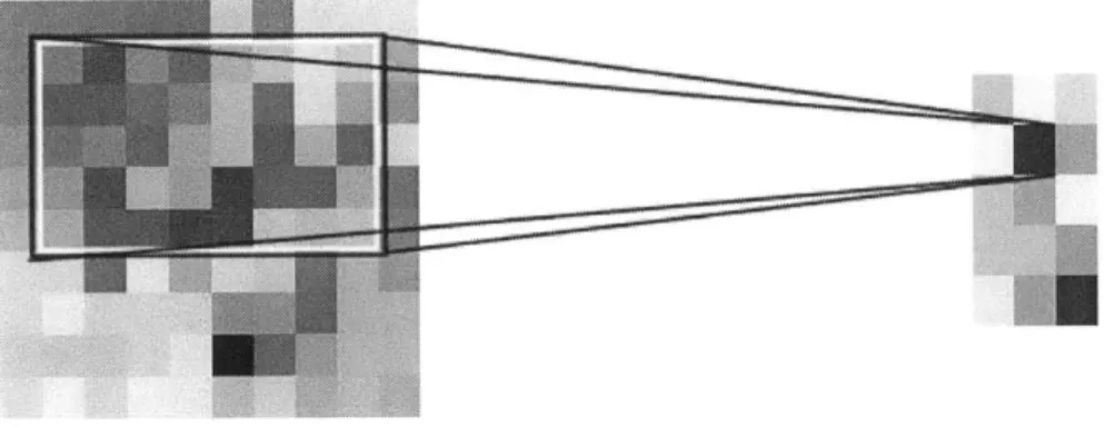
3-1 A 10 x 10 input image when fed into an 8 x 5 classifier yields a 3 x 6

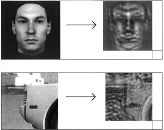
result image. The window corresponding to result image position (2, 2) is illuminated to illustrate the correspondence. . . . . 16 3-2 An 18 x 16 global classifier trained on images of the bridge of the nose

is run over two input images, one of a face and one of a non-face. Note the strong response in the vicinity of the bridge of the nose. The result images on the right are exactly 18 x 16 smaller than the input, as is illustrated by the small gray box in the lower right of each example, which is exactly the size of the classifier. . . . . 17 3-3 Top: A very simple block schematic illustrating how a global face

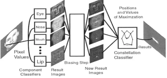
detecting system might be laid out. Bottom: A schematic for a com-ponent based classifier. . . . . 19 3-4 A block diagram schematic of the major components of our face

detec-tion system . . . . 20

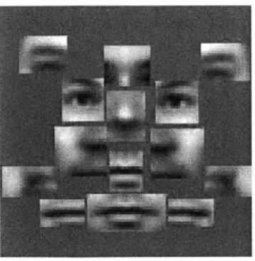
3-5 The 14 components used in our component based face detection system

arranged in a geometrically salient and vaguely disturbing pattern. . . 21

3-6 Five examples from the negative training set. The two rightmost ex-amples were drawn from larger images by bootstrapping with a weaker face detector. . . . . 21

3-7 Five examples from the positive training set. Note that the heads only turn to the right. Mirror images were used to train the full rotation between -30 and 30 degrees. . . . . 22

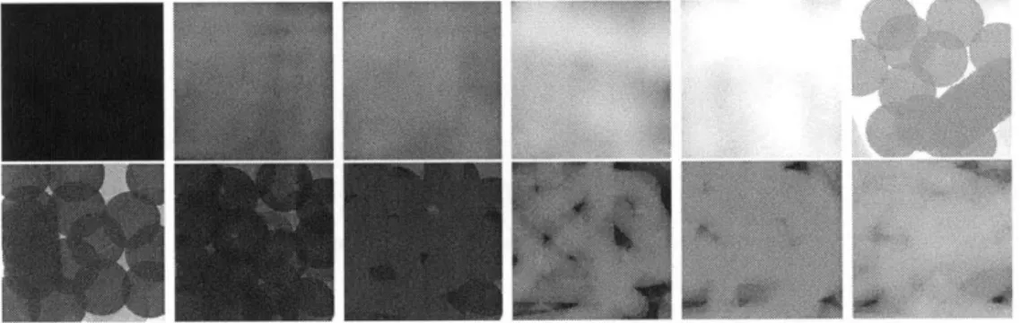
3-8 100 x 100 artificial backgrounds were used to replace the uniform blue

background in the training data. . . . . 22

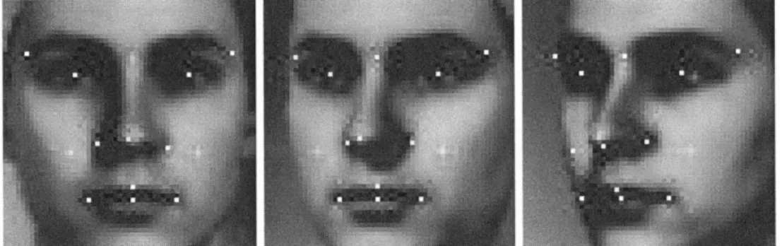
3-9 The 58 x 58 region around the face in three training images, with the 14 utilized sentinel points highlighted . . . . 23

3-10 Selected examples of the positive training set for component 0, the

bridge of the nose component . . . . 24

3-11 Selected examples of the non-face non-component training set for

com-ponent 0, the bridge of the nose comcom-ponent. . . . . 25 3-12 Selected examples of the facial non-component training set for

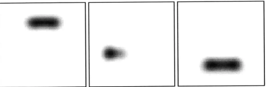
compo-nent 0, the bridge of the nose compocompo-nent . . . . 25 3-13 Position Histograms for components 0, 2, and 5. Darker pixels indicate

areas of likely location for these components . . . . 27

3-14 Pairwise position images indicate the expected position of the right eye, the left eye, and the mouth in comparison to the position of the bridge of the nose. The inner rectangle is exactly 58 x 58 for comparison. 29

3-15 Illustration of biasing Left: 11 components have correctly located,

while the right eye, the tip of the nose, and the mouth have incor-rectly located. Right: The bias image for the tip of the nose classifier. Notice that the biasing area from the 11 correct components construc-tively interfere at the expected position of the nose, while the two other incorrect classifiers weakly influence elsewhere in the image. . . . . . 30 3-16 Top: Result images for the bridge of the nose, the nose, and the right

eye. Bottom: The same result images after biasing. a was set to .5. . 31

3-17 Top: Result images for the bridge of the nose, the nose, and the right

eye when run over an image with no face . Bottom: The same

re-sult images after biasing.

a

was set to .5. Notice that without the constructive interference effects of several classifiers being in face-like geometric correspondence, the result images do not change much. . . 32

4-1 ROC curves from 14 Component classifiers tested individually on com-ponent versus non-facial non-comcom-ponent data. The comcom-ponents are in order, with component 0 on the top left, and component 3 in the top right. The solid line is the curve from the classifier trained with fa-cial negative examples. The dotted line is the curve from the classifier trained with non-facial negative examples. . . . . 36

4-2 ROC curves from 14 Component classifiers tested individually on com-ponent versus facial non-comcom-ponent data. The comcom-ponents are in or-der, with component 0 on the top left, and component 3 in the top right. The solid line is the curve from the classifier trained with fa-cial negative examples. The dotted line is the curve from the classifier trained with non-facial negative examples. . . . . 37

4-3 ROC curves from 14 Component classifiers tested individually on com-ponent versus facial non-comcom-ponent data. The comcom-ponents are in or-der, with component 0 on the top left, and component 3 in the top right. The dotted line is the curve from the classifier trained with non-facial negative examples. The solid line is the curve from the Mahalanobis classifier. Except for components 9 and 11, the SVM outperformed the M ahalanobis classifier. . . . . 38

4-4 5 example images from our positive test set, extracted from the CMU PIE database. The full size images are all between 200 and 300 pixels wide and roughly square . . . . 39

4-5 ROC curve illustrating comparative performance between a 58 x 58 linear kernel SVM (dashed line) and the full 14 component system with 5 level biasing (solid line) . . . . 40 4-6 Left: ROC curve illustrating comparative performance between the 14

component system using facial negatives in the training set (solid line) and using non-facial negatives in the training set (dashed line). Right:

4-7 Left: ROC curve illustrating comparative performance between three systems which differ only in the biasing step. These systems were built which all included the facial negative component classifiers, and the histogram based constellation classifier. 5 level biasing dashed line, 5

level biasing followed by 1 level biasing dotted line, and no biasing solid line were all tested. Right: Zoomed in view of the region between 0 and 6% of false detections. . . . . 41 4-8 Left: ROC curves illustrating comparative performance between the

systems which differ only in the constellation classifier. 4 systems were built, each of which included the facial negative component classifiers, and 5-level biasing. Dashed line: maximum value returned by posi-tion histogram measure. Solid line at top: sum of values of constella-tion which performed best in posiconstella-tion histogram measure. Dotted line: maximum value of sum of values. Solid line at bottom maximum value returned by polynomial kernel SVM. Right: Zoomed in view of the region between 0 and 10% of false detections. . . . . 42

5-1 Left: Yes Right: No. . . . . 43

5-2 In plane rotation of the image leads to incorrect eye detection due to the model of expected pairwise positions expecting near-horizontal alignm ent of the eyes. . . . . 44

5-3 Top: Error scatter plots for the left and right eye for the 2 component with geometric constraint eye-detector. Middle: Error scatter plots for the left and right eye for eye detection system which finds the full face first. Bottom: Error scatter plots for the left and right eye for the 14 component eye detection system. . . . . 46 5-4 Table of standard deviation of error in euclidian pixel distance for each

eye detector. The mean of each detector's error was near 0. . . . . . 46

Abstract

We describe the design and construction of a component based face detector for gray scale images. We will show that including parts of the face into the negative training sets of the component classifiers leads to improved system performance. We introduce a method of using pairwise position statistics between component locations to more accurately locate the parts of a face. Finally, we illustrate an application of this technology in the creation of an accurate eye detection system.

Chapter 1

Domain

The goal of the work presented here is to build an accurate face detection system for still grayscale images. The mark of ultimate success would be a system which could locate faces in images in a manner consistent with a human performing the same task. As current systems remain well behind human performance, we limit ourselves to the domain of faces which are not rotated in the image plane (around an axis through the image), and are rotated a maximum of 30 degrees left or right out of the plane (around an axis from up to down, as one looks at the image). Our system will be developed as an extension to the component based face detection system described in [8].

Chapter 2

Object Detection

Finding faces in digital images, sans color or motion cues, is a pattern recognition task. At the level of greatest abstraction, the detecting system is given an image patch of known size (or a feature vector distilled from this patch), and is to decide whether this vector stemmed from an face, or a non face. Literature concerning mathematical structures to perform such tasks, and theoretical limits on performance and error are available. The details of this branch of academia are out of the scope of this document, but the reader is invited to study the literature of learning theory, especially [20, 3, 4], for a background in statistical learning systems.

2.1

Learning From Examples

A few statistical learning algorithms are referenced often enough in this document to

warrant a coarse overview for the lay-person reader. The mathematical algorithms outlined in this section include two density based classifiers

[3]

and the Support Vector Machine (SVM) classifier [20, 2].

The basic problem is to learn a rule that divides a class of objects from a class of non-objects given examples of both sets. We begin with a set of

i

pairs (x, y) where (x E X C Rd) and (y E Y C R). For our vision task, x will represent the

feature vector stemming from an image, and y E [-1, 1] will represent whether or not this feature vector is from a target object. From the view of the pattern recognizer,

the goal is to estimate y given a new example x. We make the assumption that our data stems from two separate distributions; P(xl(y = 1)) and P(x(y = -1)); the distribution of feature vectors from images of faces, and the distribution of feature vectors from images of everything else.

A density estimation approach to classification involves attempting to model the

two distributions using the example data and the prior probability of the two classes,

P(y = 1) and P(y = -1). Using a maximum likelihood or Baysian approach, one

can choose the most likely class of a new data point

[3.

At times we will use two different types of density estimation based classifiers. In the first approach we will assume that the positive data comes from a gaussian distri-bution. By finding both the mean and covariance matrix of this distribution, we can calculate the probability that a new signal comes from the face class. We will assume for simplicity that the negative data comes from a uniform distribution, a distribution where every x is equally probable. In the implementation of this classifier, we use the simplifying assumption that the covariance matrix of the gaussian distribution is diagonal. Reasons for this assumption include the sparseness of the example data (leading to unstable models of covariance) and the speed of computation. At times we will refer to this gaussian approach, with the positive data modelled as a gaussian curve, and the negative data modelled as an even plane, as a Mahalanobis distance approach, since the weighted distance to the gaussian mean is in direct proportion to the probability density [3].

For certain classifiers, our system will use instead histograms to model proba-bility densities. Building a histogram from the training data is a simple exercise in discretizing our space of inputs into bins, and placing each example into its respective bin. Care must be taken to make the bins large enough to encompass a represen-tative number of training points from the limited training data, but not so large as to detrimentally reduce the resolution of the resulting probability density estimate. After normalizing the histogram to a volume of exactly one, given a new data point, we simply index into the histogram bin corresponding to that data point to calculate its probability. Again, because our training data is limited, in practice this histogram

based approach is limited strongly in histogram resolution when the dimensionality of the distribution is high. In our system we will use these histogram based approaches to model the 2 dimensional expected positions of facial components.

Finally, the most prevalent type of classifier we will use in this system is the SVM classifier. An SVM is a particular regularization approach to regression and classi-fication, and belongs to the class of margin maximizing classifiers. SVMs regularize between empirical loss and the smoothness of the approximating function [20, 5] and have been previously shown to work well for face detection tasks [7]. All SVM

clas-sifiers used in this work, unless otherwise noted, were trained with linear kernels and code from

[12].

2.2

Prior Work

The literature of computer vision is rich with studies of object detection. Among these studies, perhaps the most commonly selected object is the human face. The face is special because of its common appearance in visual scenes, and its simple, semi-rigid structure that varies little in geometry between samples. Even though the geometric configuration of a face is predictable, due to its 3D nature, variations in pose, illumination, texture and shape can have strong effects on the 2D projection of the face in the image plane, making the detection task difficult . Obvious application

(such as in tracking and surveillance systems) is also a likely motivation for the wealth of interest in robust automatic face detection systems.

Many early face detection systems eschewed component based architectures for a holistic approach. In [14], the distribution of faces is modelled with a mixture of gaussian curves. Faces are detected by measuring comparing novel patterns to the model distribution. A similar approach is taken in [12] and [15, 19], where a single SVM and a set of neural networks, respectively, are trained to discriminate between face and non-face patterns. In

[14,

15], virtual examples, as explored in [11], are

incorporated by rotating, translating, or scaling positive face examples, and including these new training points into the training regime in order to reduce sensitivity to

these types of variation.

It makes sense intuitively to use a part based approach to face detection if one believes that the parts of the face are less sensitive than the face as a whole to visual changes from to differences in lighting or pose. Part based systems can also be less sensitive to partial facial occlusion by interfering objects or from strong directional lighting. Perhaps the most compelling reason to continue studying part based systems is the empirical evidence supporting their accuracy over global approaches. In this section we will offer a survey of a few part based attempts at face detection. This is not to say that part based object detection schemes have been used for detecting faces exclusively. Indeed, successful implementations of component based pedestrian detectors and vehicle detectors are discussed in [13, 10] and [1] respectively.

All architectures of component based systems must at some point select which

parts to use. Some systems, such as those described in [9, 7], use features which seem

naturally salient to humans, such as the eyes, nose, and mouth. Other systems have been designed to learn object parts automatically from the training images [22, 24, 8, 23]. The system described in [8] uses 14 features that were chosen automatically using a region growing algorithm in combination with a statistical error bound [20]. In [24], an interest operator was designed to collect image patches from the training set, which were then clustered to find salient object parts. Component based object detection systems in the literature have been built with as few as 2 or as many as

150 component parts. The system described in this paper uses exactly the same 14

components described in [8] for ease of direct comparison.

Component based detection systems also differ in the type of features extracted from the images. The systems described in [16] use histogram based classifiers to judge features extracted from the wavelet decomposition of the input image. In [24], SNoW (Sparse Network of Winnows) based detectors are used to classify grayscale pixel value features. Similarly, grayscale pixel value features and SVM type classifiers are used in [8]. A completely different approach is taken in [18] where image image invariants (invariants like the bridge of the nose is brighter than the eye socket) are used. A direct comparison of feature spaces for face detection is available in [7],

the results of which suggest that compared to wavelet or first derivative of grayscale features, standard grayscale features are a good choice for frontal face detection.

Once the part examples have been located within the input image, and perhaps labelled with a confidence in each detection, each component based object detection system will use another classifier to judge whether or not the part detections are truly part of the target object, or they are simply doppelgangers stemming from similar patterns in non-object image sections. The face detection system described in [16] uses a product of probabilities, indexed from histograms, to calculate confidence in some image patch stemming from the face class. In [24], the set of part examples extracted from the image is searched for subsets geometrically consistent with actual object examples. In

[8]

only the best example of each part is used, and an SVM is utilized to decide whether the set of positions and confidences is likely to have come from a face. This SVM method of judging part detections, along with a few other top level classifiers for comparison, will be used in the system outlined in section 3.

Chapter 3

Approach

In order to best serve the reader, the discussion of the architecture of our face detection system begins with descriptions of a few more simple classifiers. This is in order to convey the concept of converting an input image into what we call a result image without the obfuscating complexity of the remainder of the component based system. We then, in section 3.2, introduce the reader to a simplified description of a component based classifier and describe how multiple classifiers are combined into a full face detection system. In section 3.3 we outline, in order of processing, the detailed internal structure of our system. Finally, at the end of section 3.3 we describe how a geometric model is fit into the face detector's architecture, and how the system is generalized to work across variations in scale.

3.1

Global Classifiers for Vision

We use the term global image classifier to describe the opposite of a component-based image classifier. These machines do not search the input image for constituent object parts as a first step toward classification. A single SVM trained on images of faces and non faces is an example of a global face detector. The features input to a global classifier do not necessarily need to be pixel values; wavelet features, first derivatives of grayscale features, and other statistics could also be used. Information such as the existence of object parts or the outputs of other object classifiers are examples

of inputs to a non-global classifier. What is the nature of a part of an object is a question best left to those more erudite than the author.

To turn a classifier into an object detector, a common strategy is to use a win-dowing technique; where every image patch is independently fed into the classifier. When the classifier output is larger than some threshold, the corresponding part of the image is labelled as being a member of the object class. It is possible build a corresponding image, separate from the input image, where the value of this new im-age at some position (i,

j)

is equal to the value output from the classifier if the input to the classifier is the image patch taken from the input image, starting at position

(i,

j);

refer to figure 3-1 for an illustration. This new image, which we will refer to as a result image will be precisely the size of the original input image, less the size of the classifier, and brighter where the classifier returned large values. Figure 3-2 illustrates the result image created when a classifier tuned to respond strongly to the bridge of the nose is run over both a face image and a non-face image. Note the strong response over the bridge of the nose. Result images will be a critical component of all systems described further in this paper.

Figure 3-1: A 10 x 10 input image when fed into an 8 x 5 classifier yields a 3 x 6 result image. The window corresponding to result image position (2, 2) is illuminated to illustrate the correspondence.

Figure 3-2: An 18 x 16 global classifier trained on images of the bridge of the nose is run over two input images, one of a face and one of a non-face. Note the strong response in the vicinity of the bridge of the nose. The result images on the right are exactly 18 x 16 smaller than the input, as is illustrated by the small gray box in the lower right of each example, which is exactly the size of the classifier.

17

3.2

Simplified Component Based Classifier

Illustrated in figure 3-3 in block diagram format is a pair of schematics depicting a global face detection system and a simple part based face detection system. In this system, which is similar to the more complicated system described in section 3.3, each component classifier operates as if it were its own global classifier. A result image is created for each component. For a face detector, there might be a result image for mouths, a result image for left eyes, etc. Once all the first level result images are created, they are used as the input to some further system which will detect faces. Here, for each window in the original image, the corresponding window in each result image is extracted. The x and y position of maximization in each of these result image patches is recorded, along with the values at the points of maximization. This

process yields a set of triplets of the form ((xo, yo, vo), (XI, Yi, v1), ... , (Xn-1, Yn-1,Vn-1))

where n is the number of facial components used by the system. This ordered set of triplets will be referred to as a constellation. For each window in the original image we extract this constellation of points where the components, or parts, fit best. This constellation is then input to another classifier, which decides between constellations stemming from faces and constellations from non-faces. The output of this upper-level classifier is recorded in the final result image. The top upper-level classifier can be of any number of types (SVMs and Baysian approaches are commonly used) and is constrained only in that it must be a function mapping valid constellations to real values.

3.3

Detailed Part Based Classifier

Figure 3-4 shows a detailed block structure diagram of our face detection system. Each sub-section will be described separately in order of data processing. The way the system searches for faces at different scales is not illustrated in figure 3-4 and will be discussed at the end of this section. The biasing, or model step between the creation of the component result images and the construction of the constellations is

Homogeneous

Face

Pixel

Classifier

Values

Eye

_{Positions and Values}

of Maximization

Nose

Class,

Pixel

Values

Component Classifiers

Results

Results

Figure 3-3: Top: A very simple block schematic illustrating how a global face detect-ing system might be laid out. Bottom: A schematic for a component based classifier.

19

optional, and will also be described at the end. Eye Nose Pixel 0 Values Lip Component Classifiers Result I mage Biasing Step New Resu s Images Positions and Values of Maximzation Constellation Classifier it

Figure 3-4: A block diagram schematic of the major components of our face detection system.

Component Classifiers.

The component classifiers are the systems, trained on different parts of the face, which compute the first set of result images from the original image. Our face detector uses the 14 parts illustrated in figure 3-5 and described in more detail in table 1. All of the parts, when situated over a frontal face, lie completely within the frame of the face and include no hairline, jawline, or ear structure. These parts were chosen in particular to match the component classifiers used in [8], which were in turn selected automatically using a statistical error bound. It would be difficult to discuss the interesting design points of the component classifiers without first discussing the training data.

3.3.1

Training Data

The training data, which was used to train the component classifiers as well as the top-level classifier, is a set of images divided into positive and negative examples of faces. The negative training data consists of 13,654 grayscale images in PPM format.

Figure 3-5: The 14 components used in our component based face detection system arranged in a geometrically salient and vaguely disturbing pattern.

to contain any faces. A few random selections from this set are shown in figure 3-6. Many, but not all of these images are difficult examples of non faces, selected by using a simple face detector to bootstrap examples out of larger images. The two rightmost negative training examples in figure 3-6 are bootstrapped examples.

Figure 3-6: Five examples from the negative training set. The two rightmost examples were drawn from larger images by bootstrapping with a weaker face detector.

The positive training data consists of 1,323 100 x 100 color PPM images of artificial head models provided through the work in [21]. A few of these are illustrated in figure

3-7. The images are of 21 different heads, which are morphs between 6 different head

models. These 21 artificial heads are viewed at 7 angles of rotation between head-on and 30 degrees to the right in 5 degree increments. At each position each head is viewed with 9 different illuminations. Copying the system described in [8], the size

of the face was decided to be 58 x 58 pixels because in the 100 x 100 images of the head, the facial part of interest is about 58 pixels square. These color images were preprocessed before using them to train the component classifiers.

Since the system described in this paper operates on grayscale images, the training

Figure 3-7: Five examples from the positive training set. Note that the heads only turn to the right. Mirror images were used to train the full rotation between -30 and

30 degrees.

data needed to be flattened into a single channel before it could be used. Also, since the background around the head was an artificial uniform field of bright blue, and a

58 x 58 box around the face at times included a bit background in rotated images,

it was decided to replace the background with the artificial patterns shown in figure

3-8. It should be noted that few of the positive examples included any of this artificial

background.

Figure 3-8: 100 x 100 artificial backgrounds were used to replace the uniform blue background in the training data.

The component classifiers must be trained on feature vectors extracted from their part of interest. In order to create the component training set, it was necessary to crop all 14 target parts out of each training image. This process was made much easier with the correspondence between images available from the artificial head data. Along with the images of the heads are included the pixel positions of 25 sentinel points on the head. Figure 3-9 illustrates the positions of some these points on a typical head model. Each of our components is defined as a sentinel point and extensions up,

see for instance that the first classifier is an 18 by 16 rectangle around a point centered at the bridge of the nose. Figure 3-10 shows a few examples of extracted training data for this classifier. When we extract the components we also extract components from the left-right mirror images of the training data. It is worth noting that when extracting a component around the left corner of the mouth in the mirror image, we must use the position of the right corner of the mouth as our sentinel point. This corpus of 2,646 images for every component comprises the positive training data of the component classifiers.

Figure 3-9: The 58 x 58 region around the face in three training images, with the 14 utilized sentinel points highlighted.

Table 3.1: Component Definitions

Index Component Description Sentinal Index Extensions left right up down

0 Bridge of the Nose 11 8 9 10 5

1 Left Eyebrow 0 3 15 8 6

2 Left Cheek 21 3 17 8 11

3 Left Corner of the Mouth 15 3 14 6 4

4 Left Eye 6 8 8 8 8

5 Upper Lip 18 6 6 6 9

6 Left Nostril 13 9 12 3 8

7 Lower Lip 16 15 15 7 7

8 Tip of the Nose 12 7 7 10 9

Table 3.1: Component Definitions

Figure 3-10: Selected examples of the positive training set for component 0, the bridge of the nose component

While exploring different avenues of improvement for this face detector, several different negative component training sets were extracted from our training data, a pair of which deserve particular mention. The first set was created in the following way. For each component classifier, a random rectangle, the size determined by the classifier, was extracted from each of the 13,654 negative training images. This will be referred to as the non-facial non-component training set, examples of which can be seen in figure 3-11. The second training set was created in the same way, but using extractions from the positive data. Care was taken so that the extractions did not overlap the canonical positions (as dictated by the sentinel position) by more than 50% of the area of the classifier. From each of the 1,323 training images 4 such rectangles were cropped out, and 4 again from the mirror image of the training

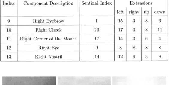
Index Component Description Sentinal Index Extensions left right up down

9 Right Eyebrow 1 15 3 8 6

10 Right Cheek 23 17 3 8 11

11 Right Corner of the Mouth 17 14 3 6 4

12 Right Eye 9 8 8 8 8

non-component training set, examples of which are shown in figure 3-12.

Figure 3-11: Selected examples of the non-face non-component training set for com-ponent 0, the bridge of the nose comcom-ponent.

Figure 3-12: Selected examples of the facial non-component training set for compo-nent 0, the bridge of the nose compocompo-nent

It is important to note here that before training any of the component classifiers described in this section, each datapoint was histogram equalized.

3.3.2

Classifier Types

Both the SVM and Mahalobonis classifier require as their input a feature vector of predefined size. For our feature space we use the grayscale values of the pixels in each training image. Grayscale pixel values have been shown to be a good feature space for frontal face detection in comparison to derivative or wavelet type features [7]. The SVMs were trained using code described in [12], but all testing was implemented in

C++ for speed.

After designing and training the classifiers, they were tested individually on com-ponents and non-comcom-ponents extracted from more artificial head data. Some real data were also labelled by hand and the data extracted so the component classifiers could be tested without the obfuscating level of the remainder of the face detection engine. The results are elaborated in the results and conclusions section (section 4).

Construction of Constellations

For each 58 x 58 window in the original image a constellation is created, as described in section 3.2. This is done by cropping the result image for each classifier to include only positions where the center of the classifier would lie within said 58 x 58 box in the original window, and recording the position of the global maximum of that crop, relative to the 58 x 58 box. Classifiers are considered to be within the window even if their area reaches beyond the edge of the window, so long as the center is still inside.

Judgement of Constellations

Once the constellation has been calculated for every 58 x 58 window in the input image, a higher level classifier is employed to judge the constellations. In the system described in

[8],

an SVM is trained on constellations from face images and non face images. This approach, and others, are compared for accuracy in section 4

Our first constellation judging algorithm uses histogram based classifiers. In this approach, we collected data from the artificial head models to produce a model of P(X,, yn

In)

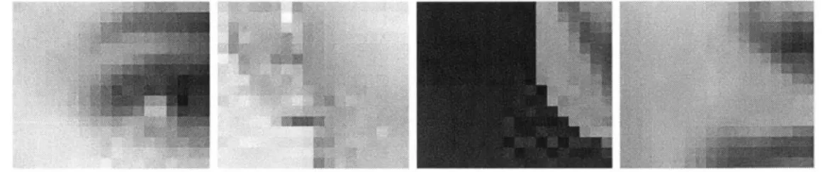
for each component, n. Figure 3-13 illustrates this position histogram for the bridge of the nose classifier, the left cheek classifier, and the mouth classifier. If we assume that the position of facial components are independent random variables, we can calculate the probability of a constellation stemming from a face by simply multiplying all the probabilities indexed from the histograms. We further assume, in this approach, that constellations arising from non-face samples are completely random, leading to a uniform probability distribution over all constellations. The position histograms were convolved with a gaussian bump of - = 2.5 pixels in order to smooth out numerical noise and make the models more tolerant to face structures unseen in our training data.

The position based histogram approach ignores the value data stored in the con-stellations, using only the position data. It is possible that discriminating information is contained in these values of maximization. Indeed, constellation classifiers using only the values were tested. Simply computing the sum of the constellation values

Figure 3-13: Position Histograms for components 0, 2, and 5. Darker pixels indicate areas of likely location for these components

was a constellation classifier tested and compared along side the histogram approach.

A few classification schemes involving simultaneously the position and the value

in-formation were also designed and tested. For instance, an SVM with a second degree polynomial kernel was trained on the constellations output from faces and from non-faces. Results for these constellation classification algorithms are elaborated upon in

section 4.

After every constellation is judged, we have available the result image for face detection, as in the more simple face detectors described above. Finding the faces in any image is now a simple task of thresholding, finding local maxima, and local suppression.

Greedy Optimization, Biasing, or Model step

One common error of the system outlined in [8] is that the classifiers don't always

maximize at the correct location. For instance the result image from the mouth clas-sifier might have a local maximum at the center of the mouth, but the peak over the eyebrow might be higher, leading to a completely wrong position in the constellation. Using only the position of the maximum stimulation unfortunately ignores that there was a strong local maximum over the correct position of the component.

We aim to assuage said problem by allowing classifiers to pass contextual informa-tion to each other. Using classifiers that have maximized in the correct posiinforma-tion, we can guess more likely positions for classifiers that were wrong. Since we don't know

which classifiers were correct a priori, we propose the following algorithm to improve the accuracy of the constellations.

First we collect the constellation, or the set of maxima from the result images, but globally instead of individually for each window. One constellation is determined for the entire image. As a side note, it is possible to collect a new constellation for every

58 x 58 window, but the biasing algorithm we will describe becomes computationally

complex (slow) and doesn't seem aid performance. In an image containing multiple faces, it might be a bad idea to collect a single constellation for the entire image. In order for the biasing step to work it is necessary that the part examples are all coming from the same face. An overlapping window technique (where the image is fragmented into sections which include at most one face) can be used to allow this type of biasing step in images with more than one face.

Once the global constellation has been determined, for every classifier i, and for

every other classifier

j

/

i,

we multiply every position in the result image of

j

by a

value representative of how likely

j

is to maximize at that location, given the location of

i.

These representative values are drawn from a histogram of pairwise position statistics. That is to say, given the position of classifier

i,

we change the result of classifier

j

to more closely model the expected position of classifier

j.

In figure 3-14 is illustrated the expected position of the right eye, the left eye, and the mouth given the position of the bridge of the nose. These values are collected from our 1,323 positive artificial training images. Again, because our data was sparse and prone to defined incremental changes in position, we convolved these pairwise position images with a small gaussian bump of u = 2.5 pixels before their use. Finally, these

histograms were renormalized to values between 0 and 1.

When running this greedy optimization algorithm we would be remiss to multiply any position in the result image by 0, or even values very close to zero, lest some classifier, perhaps one that maximized in an incorrect position, decimates the result image of another classifier in a perfectly valid position. What is needed is a type of balance between the information contained in the result images, and the contextual information shared between the classifiers. This is implemented by linearly

normal-Figure 3-14: Pairwise position images indicate the expected position of the right eye, the left eye, and the mouth in comparison to the position of the bridge of the nose. The inner rectangle is exactly 58 x 58 for comparison.

izing the values in the pair-wise position images to [(a) d, 1], where n is the number of component classifiers, and alpha is in [0, 1]. This way, the most any value in any result image can be reduced is by a factor of a, which happens only if the (n - 1)

other classifiers had a value of 0 in their pairwise position histogram at this particular point.

The intuition behind this optimization step is that often, many of the component classifiers will maximize in the correct locations, and the others will be stuck in global maxima that are far from the correct position. Assume that classifier i is one such incorrect classifier. Using our models of pairwise expected positions, the biasing areas from the set of correct classifiers will all converge at the expected position of classifier i, creating a constructive interference type effect (see figure 3-15). Ideally, after biasing the position of maximization will be under the expected position of component i if and only if there was a suitable local maximum at this position. The danger behind this type of optimization is the possibility of constellations from non-face images performing a type of automatic self assembly and being persuaded into constellations resembling those of faces. While a valid concern, as will be detailed later in the results section, section 4, empirical results show that this either does not happen, or it happens so rarely that it is irrelevant.

The greedy optimization step fits between the generation of the result images, and the generation of the constellations. Biasing takes the result images as input and

produces a new set of result images. Since the biasing step inputs result images and outputs result images, it is possible to chain biasing steps with interesting effects.

Figure 3-15: Illustration of biasing Left: 11 components have correctly located, while the right eye, the tip of the nose, and the mouth have incorrectly located. Right: The bias image for the tip of the nose classifier. Notice that the biasing area from the 11 correct components constructively interfere at the expected position of the nose, while the two other incorrect classifiers weakly influence elsewhere in the image.

N-Level Biasing

Since the individual classifiers are weak, the global maximum of some classifier Z is very often not at the correct position. Indeed, for images that are not much like our training images, it is often the 3rd or 4th ranked local maximum that is at the

correct position. As a generalization of the biasing step outlined above we present an algorithm that uses several local maxima for biasing the result images, instead of just the global maximum. The values used in the biasing step, the multipliers indexed from the pairwise position images, are retained from the previous definition.

In brief, we record the N strongest local maxima whose corresponding windows of support in the original window do not overlap at all. We then bias as before from each of these points. The collection of the local maxima is performed in a greedy iterative manner, sequentially recording the global maximum from the result image, decimating the neighborhood of this maximum, and repeating until N such local maxima are recorded.

Figure 3-16: Top: Result images for the bridge of the nose, the nose, and the right eye. Bottom: The same result images after biasing. a was set to .5.

Abstracting Across Scale

So far in the description of this system, we have been ignoring how the system detects faces at multiple scales. As it is defined right now, it will only detect faces which are exactly 58 pixels wide in the original image.

It is possible to first re-scale the input image into an image pyramid (an image pyramid is a data structure which contains multiple copies of the same image at multiple resolutions), and then run the system independently on every level of the pyramid. While simple and powerful, this method also erases one of the advantages of a component based system, the ability to detect faces where the features are slightly out of scale with each other when compared to the training images.

That said, most of the system is carried out in such a manner, one thread for each level of the pyramid. The only truly complex step is how the N-Level biasing step handles multiple scales. Rather than taking N local maxima from each level of the pyramid, N local maxima are extracted from the image pyramid as a whole. The result image multiplication step also takes place across the scale dimension. When a

Figure 3-17: Top: Result images for the bridge of the nose, the nose, and the right eye when run over an image with no face . Bottom: The same result images after biasing.

o

was set to .5. Notice that without the constructive interference effects of several classifiers being in face-like geometric correspondence, the result images do not change much.

particular local maximum is selected for biasing from level 4 in a pyramid, the result pyramids for the other classifiers are biased at not only level 4, but at corresponding positions in levels 4 ± v where v is an integer adjustable parameter of the biasing step. The effect is that a small right eye can bias a largish nose, etc.

During the constellation step, the result pyramids are handled in a in a scale-independent manner. The final output of the system, then, is actually not a result image containing bright areas where windows contain faces, but a result pyramid with similar properties.

Chapter 4

Results

The results section is arranged as follows. First we will report and compare the results from different component classifier structures and training procedures. Second we will discuss the merits of the various constellation classifiers. Finally we will illustrate the performance of our full face detection system and compare to a few other face detection systems.

4.1

Component Classifiers

In order to build a robust system, it seems intuitive that we should want the com-ponent classifiers to be as accurate as possible. Independent of the biasing and con-stellation classification step, more discrimiating component classifiers should lead to

uniform system improvement.

It was decided, then, to construct test sets for the individual classifiers by extract-ing components from more artificial data. These new head models, of which there were 1,536 images including the mirrors, were under slightly more difficult angles of rotation and more intense lighting conditions than the training data. The exact same extraction process was used to extract this data as was used to extract the training data for the component classifiers. Negative test examples were extracted as random crops from images which contained no face images. A second set of negative test examples were also drawn in a way similar to the creation of facial non-component

training set above.

It has been noted that acquiring more data to test sub-units of our system is much like assimilating additional training data. Perhaps to set a portion of our training data aside to test the component classifiers that would have been a more acceptable solution. I would argue that this situation is more like testing separate architectures than tuning model parameters.

For each component, two separate classifiers were tested. Each was trained with the SVM algorithm described above, one trained with the facial non-component train-ing set (B), and the other with the non-facial non-component traintrain-ing set (C). Both of these classifiers were tested on both test sets. 4 separate ROC curves were generated for each component, and are illustrated in figure 4-1 and 4-2.

It is expected that the classifier trained with facial negatives will outperform its counterpart on the test set with facial negatives, and vice versa. In figures 4-1 and 4-2 however, we do not see any evidence to support this trend. Instead it appears that the classifiers trained with facial non-components are slightly worse than those without, but for the most part about on par. This difference in performance can be attributed either to more variability in the negative data stemming from patterns outside of the face, or simply the larger number of data points in that set (10,584 vs. 13,654). We will see later, however, that even though the facial negative component classifiers perform more poorly by themselves, they lead to a more robust face classifier overall. Before moving away from the component classifiers we should elaborate one key point learned while conducting these tests. The component classifiers are weak in-dividually and prone to false detections, especially within the face boundary. For instance, eyebrows look like mouths, nostrils look like eyes, and the corner of the nos-tril looks like the corner of the eye. These types of confusing patterns are present in nearly every face example. Component classifiers which do not include facial negatives in their training sets are more likely to repeatedly make such mistakes.

In addition to SVM type component classifiers, Mahalanobis classifiers were also trained. Little attention has been given to them in this paper because of their poor performance. It can be seen in figure 4-3 that the SVM systems outperformed the

1 0.5 0 0 0.5 1 1 0.5 01-0 0.5 1 1 0.5

0

0

0.5 1 1 0.5 0 0 0.5 1 0.5 0 0 0.5 1 0.5

0

0

0.5 1 0.5' 0 0 0.5 1 --0.5 0 0 0.5 1 1 0.5 0 0 0.5 1 1 0.5 0 0 0.5 1 1 ₍ _ 0.5 0 0 0.5 1 1 -0.5 0 0 0.5 1 0.5 0 0 0.5 1-0.5 0 0 0.5 1

Figure 4-1: ROC curves from 14 Component classifiers tested individually on com-ponent versus non-facial non-comcom-ponent data. The comcom-ponents are in order, with component 0 on the top left, and component 3 in the top right. The solid line is the curve from the classifier trained with facial negative examples. The dotted line is the curve from the classifier trained with non-facial negative examples.

1 C 0.5 0 -0 0.5 1 0.5 0 0 0.5 1 0.5 0 0 0.5 1 1 0.5 0 0 0.5 1 1 .- -0.5 0 0 0.5 1 0.5, 0 0 0.5 1 0.5 0-0 0.5 1 0.5 0 0 0.5 1 1 -- -0.5 0 0 0.5 1 -0.5 / 0 0 0.5 0.5-0 1 /--0.5 0 0 0.5 0.5 0 0 0.5 1 1 0.5 0 0 0.5 1 0 0.5 1

Figure 4-2: ROC curves from 14 Component classifiers tested individually on compo-nent versus facial non-compocompo-nent data. The compocompo-nents are in order, with compocompo-nent

0

on the top left, and component 3 in the top right. The solid line is the curve from the classifier trained with facial negative examples. The dotted line is the curve from the classifier trained with non-facial negative examples.

slower Mahalanobis type classifier. 1 0.5 0 0 0.5 1 1 0 0.5 0 0 0.5 0.5 0 0 0.5 1 0.5 0 0 0.5 1 0.5 0 0 0.5 1 -0.5 0 0 0.5 1 0.5 0' 0 0.5 1..-0.5 0 0 0.5 1 1 -0.5' 0 0 0.5 1 -0.5 0 0 0.5 1 1 -0.5 0 1 0.5 0 0 0.5 1 -0.5 0 0 0.5 1/ 0.5 0 0 0.5 1 0 0.5 1

Figure 4-3: ROC curves from 14 Component classifiers tested individually on ponent versus facial non-component data. The components are in order, with com-ponent 0 on the top left, and comcom-ponent 3 in the top right. The dotted line is the curve from the classifier trained with non-facial negative examples. The solid line is the curve from the Mahalanobis classifier. Except for components 9 and 11, the SVM outperformed the Mahalanobis classifier.

4.2

Face Detection

Although the system was trained on artificial data, it was decided that for face de-tection it should be tested on real images of faces. The positive test data were drawn from the CMU PIE database available at [17]. In order to save time computationally, the heads were cropped out by hand before testing. The CMU PIE database includes

removing from the data all heads at rotations out of the plane more than 30 degrees, we were left with a positive test set of 1,834 images, examples of which are illustrated in figure 4-4.

Figure 4-4: 5 example images from our positive test set, extracted from the CMU PIE database. The full size images are all between 200 and 300 pixels wide and roughly square

The negative test data, like the negative training data, were extracted from images containing no faces. This data was also bootstrapped out of the image set using a simple face classifier and choosing examples which look like faces, in order to make the test difficult. The classifier used to extract these test examples was not the same classifier used to extract the difficult training examples. In total, 8,848 images comprised the negative test set.

When each image is passed through the face detection system outlined in section

3, we are left with a corresponding result pyramid. This pyramid should contain

strong values at locations corresponding to subwindows that look, to the system, like faces. For each image in the test data, we recorded only the strongest response in the result pyramid, and used this to build an ROC curve.

The ROC curve in figure 4-5 is the curve gleaned from running our system using the component classifiers trained with negative examples drawn from the rest of the face. The images were tested for faces at every scale from 60 x 60 to 110 x 110 in 11 geometric increments. Biasing was performed using 5 local maxima per component and then again once globally . The dashed line below, for comparison, is the result

from a linear kernel SVM trained on the full 58 x 58 facial extractions from the exact same training data.

In figure 4-6 we again see the same solid curve. The dashed line is now the exact same system as above, with the component classifiers replaced with component

0.9 0.8 -0.7 -0.6 0.5 , 0,3-0.2 0.1 0 0.1 0.2 0.3 0.4 0.5 0.6 0.7 0.8 0.9 1

Figure 4-5: ROC curve illustrating comparative performance between a 58 x 58 linear kernel SVM (dashed line) and the full 14 component system with 5 level biasing (solid line)

classifiers trained on non-facial negatives. The two systems are about on par in this performance measure, however, in the graph on the right, it can be seen that in the region of interest, the classifier with the facial negative trained component classifiers is outperforming its peer by about 5% to 10%. The face detector performs better with the facial non-component trained component classifiers, which individually performed worse.

Figure 4-6: Left: ROC curve illustrating comparative performance between the 14 component system using facial negatives in the training set (solid line) and using non-facial negatives in the training set (dashed line). Right: Rescaled view of the graph on the left

In figure 4-7 are ROC curves for three systems which differ only in the biasing 09 -0 0.8 0 0. 0.7 0. 0.6 -0. 0.5 _0. 0.4 0. 0.3 0. 0.2 0. 0.1 _0. 0 0.1 0.2 0.3 0.4 0.5 0.6 0.7 0.8 0.9 1 9-1 6 5 4 - 3- 2-0 0.01 0.0 0.03 0.04 0.05 0.06 0.07 0.0

step. The solid curve near the bottom is from a system which is using no biasing at all; the results from the component classifiers are directly converted into constellation maps, which are then classified by our position histogram based constellation clas-sifier. Performance is increased greatly (as much as 50%) by using a 5-level biasing routine on the result images before collecting the constellations. Earlier a suggestion was made that biasing steps can be chained together. The system which genereated the dotted curve uses first a 5-level biasing step and second a 1-level biasing step before the constellations are created. The reduction in performance is perhaps due to forcing the negative examples into constellations which look like they came from faces. 009 "s, . 0.0-0.8- 0.8-0.7 / 0.7 -0.6

/0.6

05 _0.5 0.41 _0.4-/ 0.3 0.3- 1_ 0.2 _0.2 0 1O 0.2 0.3 0.4 0 0.6 O 0.7 0 .8 0.9 1 0 0.01 0.02 0.03 0.04 0.05

Figure 4-7: Left: ROC curve illustrating comparative performance between three systems which differ only in the biasing step. These systems were built which all included the facial negative component classifiers, and the histogram based constel-lation classifier. 5 level biasing dashed line, 5 level biasing followed by 1 level biasing dotted line, and no biasing solid line were all tested. Right: Zoomed in view of the region between 0 and 6% of false detections.

Figure 4-8 illustrates the results from a direct comparison of systems which differ only in the constellation classifier. This figure shows performance on the test described above for 4 different face detection systems, each of which use the same component classifiers, biasing scheme, and scaling. In order to save time, only every third image in the negative test set was used, leaving the same 1,834 positive test points, but only

2,949 negative test images. The dashed curve at the top was created by a system using

the position histogram constellation classifier. Moving downward in performance, 41

the solid curve underneath was created by recording the sum of the values in the constellation which performed best in the histogram measure. This means that every constellation from the input image was judged by the histogram measure. The sum of the values in this constellation was recorded instead of the value returned by the histogram classifier. The system which created the dotted line recorded the sum of values from the constellation with the largest sum of values. Finally, the solid curve at the bottom was created by training a second degree polynomial kernel SVM on the constellations created by running the component classifiers back over the training data. The unexpectedly weak performance from this classifier might be due to the limited training data used to collect the constellations.

0.9 - . 0.9 - - - ----0.8 I 0.8-0.7 .0.8-0.7 0.6 - 0.6-0.5 -0.5 -0.4 04 0.3 -0.3 -0.2 -0.2- _I 0 0.1 0.2 0.3 0.4 0.5 0.6 0.7 0.8 0.9 1 0 0.01 0.02 0.03 0.04 0,05 0.06 0.07 0.08 0.09

Figure 4-8: Left: ROC curves illustrating comparative performance between the sys-tems which differ only in the constellation classifier. 4 syssys-tems were built, each of which included the facial negative component classifiers, and 5-level biasing. Dashed line: maximum value returned by position histogram measure. Solid line at top: sum of values of constellation which performed best in position histogram measure. Dotted line: maximum value of sum of values. Solid line at bottom maximum value returned

by polynomial kernel SVM. Right: Zoomed in view of the region between 0 and 10%