HAL Id: halshs-00096936
https://halshs.archives-ouvertes.fr/halshs-00096936v2
Preprint submitted on 20 Sep 2006HAL is a multi-disciplinary open access archive for the deposit and dissemination of sci-entific research documents, whether they are pub-lished or not. The documents may come from
L’archive ouverte pluridisciplinaire HAL, est destinée au dépôt et à la diffusion de documents scientifiques de niveau recherche, publiés ou non, émanant des établissements d’enseignement et de
Behaviors and housing inertia are key factors in
determining the consequences of a shock in
transportation costs
François Gusdorf, Stéphane Hallegatte
To cite this version:
François Gusdorf, Stéphane Hallegatte. Behaviors and housing inertia are key factors in determining the consequences of a shock in transportation costs. 2006. �halshs-00096936v2�
Behaviors and housing inertia are key factors
in determining the consequences of a shock in
transportation costs
Fran¸cois Gusdorf
a,b, St´ephane Hallegatte
c,b,1aCentre International de Recherche sur l’Environnement et le D´eveloppement,
Paris, France
bEcole Nationale des Ponts-et-Chauss´ees, Paris, France cCenter for Environmental Sciences and Policy, Stanford, USA
Abstract
This paper investigates the consequences of a sudden increase in transporta-tion costs when households behaviors and buildings inertia are accounted for. A theoretical framework is proposed, capturing the interactions between behaviors, transportation costs and urban structure. It is found that changes in households consumption and housing choices reduce significantly the long-term adverse effects of a shock in transportation costs. Indeed, the shock translates, over the long-run, into a more concentrated housing that limits households utility losses and main-tains landowners’ income. But, because of buildings inertia, the shock leads first to a long transition, during which the adjustment is constrained by a suboptimal housing-supply structure. Then, households support larger losses than in the final stage, though lower than with no adjustment at all, and landowners experience a large decrease in their aggregate income and an important redistribution of wealth. Negative transitional effects grow as the shock becomes larger. Thus, behaviors and buildings inertia are key factors in determining the vulnerability to transportation price variability and to the introduction of climate policies. Our policy conclusions are that: (i) if a long-term increase in transportation costs is unavoidable because of climate change or resource scarcity, a smooth change, starting as early as possible, must be favored; and (ii) fast-growing cities of the developing world can reduce their future vulnerability to shocks in transportation costs through the implementation of policies that limit urban sprawl.
1 Introduction
In four years, between 2002 and 2006, energy prices have soared in the U.S., following the rapid increase in the price of crude-oil, from between 20 and 30 a barrel over the last decades to more than 60 in the last months. As a consequence, U.S. gasoline prices have doubled over a couple of years, from their average values of approximately 1.50 a gallon to their mid-2006 values, reaching 3 a gallon in some U.S. states. Compared with the lifetime of the equipments that drive energy consumption, like transportation infrastructure and buildings, this increase has been extremely rapid, justifying the term of energy shock. Also, with 87.9 percent of the Americans driving to commute ev-eryday (Reschovsky, 2004), gasoline prices have a direct and strong influence on households budgets. Transportation expenditures constitute the second-largest expense category of American households, with 19.3 percent of their budget devoted to these expenditures (O’Toole, 2003). Thus, even though cur-rent prices have already been reached in constant dollars in the late seventies, consequences on welfare of such a shock in transportation costs are far from negligible, explaining the growing public concern about this issue.
Reducing this social vulnerability to oil-price variability, and mitigating cli-mate change, can be done through reductions in oil consumption. Today, there-fore, heated debates are going on about the necessity of much higher gasoline prices to promote energy conservation and innovation in renewable and clean energies. But while the long-run benefits associated with such a policy are unquestioned, some argue that its short-term costs would be unbearable. The main underlying question behind this debate is about the timing of actions: policies aiming at reducing oil consumption can be either immediate or de-layed, in the wait for new technologies to appear; they can also be either progressive or aggressive. Obviously, reaching a given long-term target can be done through delayed and aggressive policies, or, starting sooner, through smoother implementation paths. This trade-off between the timing and the ag-gressiveness of measures is key in the design of energy policies (e.g., Weyant, 1993; Hourcade and Robinson, 1996; Ambrosi et al., 2003).
To provide new insights into the design of such policies, this paper investigates the determinants of energy-shock consequences. Our intuition is that largely spread-out cities like Los Angeles, which have been developed recently and in response to low transportation costs, would suffer from a rapid increase in these costs more than concentrated cities, which have been developed in
Email addresses: gusdorf@centre-cired.fr (Franc¸ois Gusdorf), hallegatte@centre-cired.fr(St´ephane Hallegatte).
1 CIRED, 45bis Av. de la Belle Gabrielle, F-94736 Nogent-sur-Marne, France. 2 CIRED is a EHESS-CNRS-ENPC-ENGREF laboratory.
response to higher transportation costs. Our paper is, therefore, based on the ideas that (1) housing and localization choices will play a key role in determin-ing the consequences of a price change, and that (2) the urban structure and the timescale of the change are among the main drivers of the welfare losses due to an increase in transportation costs. In particular, as already stressed by Weyant (1993), the timescale of an energy-price change has to be compared with the inertia of the technico-economic system. Indeed, a slow increase in energy prices would let time for productive capital and infrastructures to ad-just to new prices, leading to limited losses. Meanwhile, an instantaneous (or quasi-instantaneous) shock in energy prices would make all equipments and infrastructures ill-adapted. Since, those infrastructures drive energy consump-tion, their ill-adaptation would make behavior changes less efficient to limit welfare losses. A shock, therefore, would cause much larger damages than a smooth transition. Akerman and Hojer (2006) mention this ill-adaptation as an important problem, but they do not attempt to evaluate its negative ef-fects. To do so, this paper focuses on the largest pieces of infrastructure in developed countries, namely the buildings in urban environments, whose value constitutes more than 50 percent of the installed capital’s value (Greenwood and Hercowitz, 1991), and whose annual depreciation rate is very low4. We
carry out modeling experiments to see how the assessment of welfare losses due to an increase in transportation costs changes when this buildings inertia is taken into account.
The paper is organized as follows: Section 2 presents a standard urban eco-nomic modeling a la Von Thuenen (1826). This modeling framework was adapted to urban economics by pioneering works of Alonso (1964), Mills (1967), and Muth (1969). We also introduce the representation of housing infrastructure as first introduced by Muth (1969). These models, widely used in standard microeconomic urban theory, provide us with a common frame-work allowing to understand the involved mechanisms and their consequences on welfare. Section 3 introduces the transportation cost shocks and makes the model able to take into account the existence of different timescales in the dynamics of cities, from the adjustment of housing choices by households to the slow adaptation of urban structures. More precisely, we focus on the timescale of a few decades: it is short enough to neglect building turn-over; it is long enough to allow for an adjustment of households housing choices, though constrained by the existing housing supply5. This section presents
model estimates of the additional welfare losses due to buildings inertia. Fi-nally, Section 4 concludes by providing some insight into policy issues and by suggesting future researches.
4 For instance, Jin and Zeng (2004) found an annual depreciation rate of 1.54%. 5 We are not, therefore, investigating the very short term like Noland et al. (2006),
2 Model
According to standard urban economic theory, transportation prices influence households behavior and, thereby, the size of a city, as well as its structure, e.g. its density gradient. Few empirical studies, however, investigate this influence. Among them, Brueckner and Fansler (1983) found no evidence of such an influence but McGrath (2005) questioned the transportation prices estimates used by Brueckner and Fansler. Using improved data, he found a significant negative link between transportation prices and urban sprawl, concluding that “The negative significance of the transportation cost variable (...) indicates that the adoption of policies that directly impact private transportation costs, such as congestion tolls and fuel taxes, can have a direct impact on urban scale”. Yacovissi and Kern (1995) studied density and buildings heights, and found empirical evidence consistent with standard urban economics modeling.
Based on this theory, our model aims at representing the interaction between transportation prices, households and landowners’ behaviors, and housing in-frastructures. Most of the literature in standard urban macroeconomics as-sumes that the city situations correspond to a long term equilibrium, where housing capital is fixed. Some papers have dealt with housing capital mal-leability. Brueckner (2000) provided a survey of this literature, originating with Evans (1975) and Fisch (1977). Published articles focused on the dis-crete process of destruction and construction of buildings and on the influence of historical factors on this process (e.g., Capozza and Li, 1994). But, to the best of our knowledge, no paper investigated the influence of a shock in trans-portation prices. Also, previous works did not take into account households moves within existing buildings. Thus, they did not analyze the medium-term effects of a transportation shock, which is, however, very important in pol-icy design. Our model is built to capture also this intermediary period and improve our understanding of energy-shock consequence on this timescale.
2.1 The Monocentric Closed City Model
In our framework, the city has a single center, the central business district (CBD), and has a circular symmetry around this center, so that any position in the city can be defined by the distance from the CBD. Housing infras-tructures throughout the city can be either exogenous or endogenous. In the latter case, we use a construction function a la Muth (1969), to represent the characteristics of housing structures. The city is assumed to be closed, i.e. the number of households is exogenously fixed.
landowners. Households rent apartments from landowners, who own the land and the buildings. This distinction is useful for the analytical process. Four goods are available in the economy: land (s), capital (k), composite good (z), and housing service (q). Housing service consists in the number of square meters of housing, and related goods and services whose consumption changes with this surface (heating, electricity, etc).
2.2 The households
Households choose their housing location and consumption bundle to maxi-mize their utility. We will suppose here that housing service supply is exoge-nously given by a supply function H(r), which is null for r > rf, where rf is
the size of the city.
Each household is composed of one worker commuting every day to the CBD. All workers earn the same income Y , and enjoy utility from a composite good z and a housing service q. All workers share the same utility function U (z, q).
Each worker chooses his/her housing location r in the city, where the unit price of housing service at location r is RH(r). He/she maximizes his/her
utility level under a budget constraint. The behavior of a worker living in the city is given by:
maxr,z,q U (z, q) (1)
s.t.
z + RH(r)q ≤ Y − T (r) (2)
where Eq. (2) is the budget constraint of the representative household if it chooses to live at distance r, while T (r) represents the transportation costs of commuting. Those transportation costs are indeed generalized transportation costs, i.e. they take into account the cost of transportation itself as well as the loss of time spent in commuting, that could have been devoted to work or leisure. Marginal transportation cost is assumed to be constant, and no congestion is taken into account.
We define the housing bid-rent functions ψH(r, u), which depends on the
dis-tance r and the utility level u:
ψH(r, u) = maxq≥0
Y − T (r) − Z(q, u)
where Z(q, u) is such that U (Z(q, u), q) = u; we assume that this number exists and is unique. Intuitively, ψH(r, u) is the maximum rent per unit of
housing service that a consumer can afford if he wants to achieve an utility level u at a distance r.
Classically, competitive equilibrium leads in each period to a situation where:
• there is no utility difference between consumers earning the same income:
all consumers throughout the city have the same utility level u (4)
• the housing rent curve throughout the city stems from this utility level u as follows:
at all r, RH(r) = ψH(r, u) (5)
Setting rf as the limit of the city, beyond which no consumer lives, and n(r) as
the density of consumers per square meter of land at distance r, equilibrium conditions are then:
RH(r) =
ψH(r, u) = maxq≥0 Y −T (r)−Z(q,u)q for r ≤ rf
0 for r ≥ rf (6) n(r) = H(r)/q(r, u) for r ≤ rf 0 for r ≥ rf (7) N = rf Z 0 n(r)dr (8) ψH(rf, u) ≥ 0 (9)
Definition 1 (CSEx) : for a given set of parameters, N , Y , p, and for given functions H(r) and T (r), a competitive static equilibrium with exogenous hous-ing density (CSEx) is characterized by the existence of variables and functions u, rf, n(r), RH(r), q(r), and z(r) verifying Eqs. (6) to (9).
2.3 The landowners
In the section above, we did not specify the profile of the housing supply H(r), which was supposed exogenously given. However, we want this housing supply to be endogenous in our long-term model. To do so, we define a competitive
equilibrium with endogenous housing structure, which arises from the behavior of landowners.
At each location, each absentee landowner allocates his/her amount of land L to agricultural use or to residential use. In the first case, the rent drawn from the land will be RaL, where Rais the fixed agricultural rent. In the second case,
the landowners invests in housing capital K to produce a housing service H, measured in terms of inhabitable surface (in square-meters). The production function H = F (L, K) gives the amount of housing services produced from an amount L of land and an amount K of capital. Function F is assumed to have constant returns to scale. Considering the rent level as exogenously given, each landowner chooses the amount of capital he/she invests, in order to maximize his/her profits. Thus, the behavior of an absentee landowner, owning land surface L at location r, is given by:
maxK 1
1 − σ[RH(r)F (L, K) − ρK] (10)
where RH(r) is the unit price of housing service at location r; rent revenues are
discounted on an infinite time by the factor σ; and the capital is borrowed at an interest rate ρ. Landowners build very long term housing infrastructures, and they expect to be paid the same rent every year, i.e. until discounting makes revenues be negligible.
The landowner chooses in fact the capital to land ratio x = K/L. Since F has constant returns to scale, this ratio does not change with the surface of land that is owned by an individual landowner; it depends only on distance r. We can use f (x) = F (L, K)/L as a proxy for housing density, or building’s height, and define:
x∗
(r) = arg max
x [RH(r)f (x) − ρx] (11)
As a consequence, the limit of the city is endogenously defined as follows:
rf = max[r, RH(r)f (x∗(r)) − ρx∗(r) ≥ Ra] (12)
As the production function has constant returns, this individual behavior can be aggregated at each location in the city. The optimal housing investment K∗(r) corresponds to a capital to land ratio x∗(r), and leads to a total
pro-duction of housing services at the distance r:
H(r) = Land(r) · f (x∗(r)) for r ≤ r f 0 for r ≥ rf (13)
where Land(r) is the surface of available land at location r.
Furthermore, at the city limit:
RH(rf)H(rf) − ρK∗(r) = RaLand(rf) (14)
We define the housing service density h(r), as the ratio of the inhabitable sur-face at a location r to the total amount of available land: h(r) = H(r)/Land(r) = f (x∗(r)). If q is the quantity of housing service per household at location r,
and s and k are respectively the quantity of land input and capital input per household, then: n(r) = H(r) q(r) = F (L(r), K(r)) q(r) = L(r) s(r) = K(r) k(r) . (15)
Thus, we immediately get s = qL/F (L, K) and k = qK/F (L, K). Since F has constant returns to scale, q = F (s, k).
Definition 2 (CSEn) : for a given set of parameters N , Y , RA, p, and for
given functions Land(r), T (r) and F (L, K), the competitive static equilibrium with endogenous housing density (CSEn) is reached in the city when one can find parameters and functions u, rf, n(r), RH(r), z(r) and H(r) verifying
Eqs. (6) to (14).
To investigate the distributive effects of policies, we introduce the Local Land Income (LLI), which is the income generated by a square meter of land when the investments described by Eq. (10) have been done. Formally:
LLI(r) = RH(r)f (x∗(r)) − ρx∗(r) (16)
The variable LLI(r) is, indeed, an index of the value of one square meter of land, since it measures the income generated by this area.
We also define the Aggregate Landowners’ Income (ALI), which derives intu-itively from its local version LLI(r):
ALI =
rf
Z 0
Land(r)LLI(r)dr (17)
We finally define the Aggregate Invested Capital (AIC), which measures the total amount of housing capital invested by landowners, and the Aggregate Housing Rent (AHR), which is the sum of all rents paid by households to landowners:
AIC = rf Z 0 Land(r)K L(r)dr AHR = rf Z 0 RH(r)H(r)dr
Thus: ALI = AHR − ρAIC
While LLI(r) allows to track distributive effects between landowners owning land at different distances from the CBD, the variable ALI shows how policies affect landowners as a group.
2.4 Static Equilibrium
2.4.1 Specific Functional Forms and Calibration
Having defined a theoretical analysis framework in the preceding section, we now intend to analyze the specific features which are of interest for this paper. Thus, we turn to specific functional forms so as to explore the properties of our model. We assume that the utility function and the housing service production function are given by:
U (z, q) = zαqβ where α, β > 0 and α + β = 1
F (s, k) = Asakb where a, b, A > 0 and a + b = 1 (18)
These Cobb-Douglas functions are widely used for exploratory studies, as in Mills (1972), Brueckner (1980) or Fujita (1989). For simplicity’s sake, we also assume that transportation costs increase linearly with distance, T (r) = pr, that the amount of available land is proportional to the distance from the CBD, L(r) = lr, and that the agricultural rent is null, i.e. Ra= 0.
We calibrated the main parameters so that the city on which we carried numer-ical analysis should approximate Los Angeles county. Therefore, 4, 3 millions workers live in this city, earning a $20 700 yearly income (data U.S. Cen-sus Bureau 1999). The transportation price is calibrated using 1999 gasoline prices (i.e. 32 cents per km on average, data American Automobile Associ-ation 1999). For this calibrAssoci-ation, we do not take into account the value of time in transportation costs. Neither did we consider congestion costs, and the existence of amenities specific to certain locations. As a results, the city
we represent is very simplified. Maximum commuting distance is 88 km, and 90% of the inhabitants of the city are at a distance from CBD that is inferior to 45 km (figures of numerical simulations will represent what happens inside this perimeter, distances from the CBD being expressed in km). Besides, in a Cobb-Douglas utility function as described in Eq. (18), coefficient β represents the share of households budget devoted to housing (and related expenses, as housing equipment, heating, ...) at the equilibrium. Empirically, this share proves to be very stable, close to 25 %. Concerning the construction function, we lack robust empirical evaluation; thus, we tested a very wide range of pa-rameter values. The numerical analyses we present here were carried out using a = 0.5. Systematic sensitivity analyses have been carried out, and all quali-tative results of the model are not changed in a reasonable range of parameter values.
In the following, we focus on the influence of the transportation price p on model equilibrium. We describe this influence first on the city structure, then on households and finally on landowners.
2.4.2 Structure
We present in this section the characteristics of a CSEn in our modeling frame-work, calibrated on the city of Los Angeles, CA. Classically, it provides a static equilibrium, whose features reproduce commonly observed urban characteris-tics; see for instance McGrath (2005).
Figure 1 shows the rents RH(r) and the housing service per capita q(r), with
respect to the distance from the CBD and for two values of the transporta-tion price: p = 32 cent per kilometer, which is the estimate by the American Automobile Association for 1999; and twice this price, 2p, to assess the sen-sitivity of the model to changes in the transportation price. For each price, Fig.1 shows how the rents decline with distance, while consumption of hous-ing service per capita increases. Households livhous-ing far from the center live in bigger flats or houses, where rent levels are cheaper. They can afford high commuting costs, and achieve the same utility level as those located close to the center. The larger the transportation price p, the greater is the gradient of rents and housing service per capita.
Figure 2 shows the housing structure corresponding to the two different trans-portation prices p and 2p. The left panel shows the housing density throughout the city h(r), which decreases with respect to the distance from the city center: landowners react to higher rent levels and invest in bigger buildings close to the CBD. Housing supply H(r), however, decreases to zero when the distance ap-proaches zero, although buildings height at the CBD is at its maximum. This is due to the fact that, in a circular city, land becomes scarcer and scarcer as
0 0.5 1 1.5 2 0 5 10 15 20 25 30 35 40 45 distance r RH(p,r) RH(2p,r) 0 1 2 3 4 5 6 7 8 0 5 10 15 20 25 30 35 40 45 distance r q(p,r) q(2p,r)
Fig. 1. Rent curve RH(r) (index RH(p, 0) = 1) and per capita housing service
consumption q(r) (index q(p, 0) = 1), with respect to the distance from the city center, at equilibrium. The different curves correspond to transportation prices p and 2p. 0 0.5 1 1.5 2 0 5 10 15 20 25 30 35 40 45 height index distance r h(p,r) h(2p,r) 0 0.5 1 1.5 2 0 5 10 15 20 25 30 35 40 45 surface index distance r H(p,r) H(2p,r)
Fig. 2. Housing structures corresponding to two different transportation prices, with respect to the distance from the CBD (left: index h(p, 0) = 1; right: index H(p, 5) = 1).
the distance from the CBD tends to zero.
When the transportation price p increases, the repartition of investment through-out the city is driven by the fact that households living close to the CBD have much less commuting to pay for than other households; therefore, housing ser-vices close to the CBD become more wanted as transportation costs increase; this effect concentrates households towards the city center, where their hous-ing budget is higher. As a consequence, competition for houshous-ing gets fiercer close to the CBD, and decreases far from the CBD. When p increases, it makes buildings close to the CBD higher, and those far from the CBD smaller.
0.7 0.75 0.8 0.85 0.9 0.95 1 1.05 1.1 0.4 0.5 0.6 0.7 0.8 0.9 1 1.1
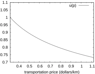
transportation price (dollars/km) u(p)
Fig. 3. Equilibrium level of households utility u (index u = 1 for p = 0.32 dollars per kilometer), as a function of the transportation price p.
2.4.3 Households
It can be shown (see Appendix) that any transportation price p is associated with one unique utility level u, satisfying:
uγ+1 = lB N (γ + 2)
Yγ+2
p2 (19)
In this equation, the land availability, described by the parameter l, influences utility directly: with more land to build on, consumers have more housing service available in locations where transportation costs are low, and their utility is higher. A larger number of inhabitants N lowers utility, because more people would then compete for a limited amount of land. On the other hand, utility increases strongly with income Y . This is because transportation costs at a given location are fixed and, as income increases, they represent a smaller part of consumers’ budget.
Most importantly, transportation price p has a large, and negative, influence on equilibrium utility. Figure 3 shows the rapid decrease of utility as trans-portation price increases.
2.4.4 Landowners
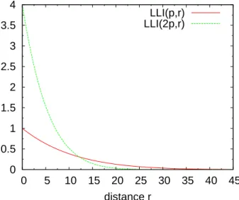
As shown by Figs. 1 and 2, both the rent curve and the housing density de-crease with distance r. Those two evolutions have opposite effects on Landown-ers’ income. However, one can show analytically that LLI(r) unambiguously decreases with distance r. Furthermore, as illustrated by Fig. 4, an increase in
0 0.5 1 1.5 2 2.5 3 3.5 4 0 5 10 15 20 25 30 35 40 45 distance r LLI(p,r) LLI(2p,r)
Fig. 4. The variable LLI(r) is the income generated by a square meter of land at location r. The two curves correspond to transportation prices p and 2p (index LLI(0, p) = 1).
the transportation price concentrates landowners’ income towards the CBD, i.e. the income of landowners close to the center increases, while the income of those located far from the center decreases.
At the aggregate level, since any household in the city will devote a fraction β of its budget Y − pr to housing, we have:
AHR = rf Z 0 β(Y − pr)n(r)dr = N a Y γ + 3 (20)
Using Eq. (20), and Eqs. (25), and (26) from the Appendix, the value of Aggregate Invested Capital, is given by :
AIC = rf Z 0 Land(r) ·k s(r)dr = b a N Y γ + 3 1 ρ (21)
The Aggregate Housing Rent AHR and the Aggregate Invested capital AIC are proportional to N and Y . Indeed, the higher the income, and the more people live in the city, the higher is the rent at the aggregate level. More precisely, as N increases, the city limit does not change but the buildings are higher6; as Y increases, buildings get bigger and the city expands outwards.
6 This is formally true only in the special case where R
a = 0. However, in our
modeling exercises, changes occurring when Ra > 0 are negligible compared with
More important is the fact that the Aggregate Housing Rent AHR and the Aggregate Invested Capital AIC are independent of the transportation price p. If it increases, consumers’ housing budgets become smaller. But more peo-ple live close to the CBD, where commuting expenses are also smaller. The combination of these effects lets the AHR unchanged (see Eq. (20)). Because buildings are higher close to the CBD, and smaller far from it, exactly the same amount of capital is invested at the aggregate level, and AIC is also in-dependent of p (see Eq. (21)). As a consequence, the Aggregate Land Income ALI is also insensitive to changes in transportation costs.
Therefore, an increase in transportation price does not change the income of landowners as a group, but leads to a large redistribution of income among landowners, since the land close to (resp. far from) the CBD can generate more (resp. less) rent when transportation prices are higher (see Fig. 4). In other terms, the value of land at different locations changes in response to transportation price variation, even though the return on equity of building investments is kept unchanged through the adjustment of the amount of in-vested housing capital. Also, p influences strongly rf = Y /p and, as p increases,
the surface inside the city decreases: some landowners choose to use their land for agricultural activity instead of housing7.
2.4.5 Summary
These results show that, over the long-term, the city structure, the households utility, and the distribution of wealth among landowners depend on trans-portation costs. The city structure is adapted over the long-term to a specific price. However, the adaptation of the housing supply cannot be instantaneous. As a consequence, if a shock occurs on transportation price, the subsequent ill-adaptation of the city structure will generate a new situation, that needs to be taken into account in the design of transportation policies. To investigate this issue, the following section will consider an exogenous shock on trans-portation price and look at the influence of the city structure ill-adaptation on medium-term welfare losses.
the results in a qualitative manner, while it makes the demonstration much more complex. These change are, therefore, disregarded in this paper.
7 This mechanism is formally true only if R
a = 0. If this is not the case, i.e. if
Ra > 0, then AHR and AIC change with transportation price p. Here also, the influence of Ra is of second-order and is, therefore, neglected.
3 Transportation price shocks
In this section, we consider a shock in transportation costs, with the trans-portation price that abruptly jumps from an initial value pi to a final value
pf. When the transportation price increases suddenly, the instantaneous
conse-quence is an increase in aggregate transportation expenditures for households, at the expense of the consumption of composite goods. For instance, a doubling in the price of transportation per km decreases the aggregate consumption of composite by 29 percent if households do not change their housing choices. Thus, energy policies that would lead to a large increase in transportation costs are often considered unbearable.
However, households will rapidly adjust their behavior to the new price, to avoid as much as possible utility losses. As we shall see, the efficiency of this adjustment depends on whether buildings inertia is taken into account. We focus here on medium- to long-term timescales, from one decade to a few cen-turies. Over this timescale, households consumption bundles and localizations have enough time to adjust to transportation cost changes, but, because of the long lifetime of buildings, housing-supply structure can be considered un-changed. Also, considering this timescale allows us to represent increases in transportation costs, like the recent increase in gasoline price over four years in the U.S., as instantaneous shocks.
We consider three periods. (1) The initial period, before the shock, during which the city is assumed to be at its long-run equilibrium. (2) The final pe-riod, which takes place a long time after the shock, at least several decades, and during which the city is at its new long-run equilibrium, fully consistent with the new transportation price. And, (3) an intermediary period, the medium period, which takes place approximately between one decade after the shock and a few decades after the shock. During this medium period, the housing-supply structure is not adapted to the new transportation price, because of the long adjustment delay in buildings and city structure. Households, on the other hand, have adjusted their behavior to the new transportation price and the available housing infrastructure. Corresponding variables and parameters will be characterized by a subscript i, f , or m.
In the following, households and landowners adopt a myopic behavior. In the initial period, they do not anticipate the shock, and make their decisions as if pi should not change.
3.1 No Inertia
The effect of a shock when no buildings inertia is taken into account can be very simply derived from Section 2.4. We explore here only two stages: the initial and final periods, disregarding the transition between them. With the functional forms we specified, we can characterize the long-term equilibriums of the city, with endogenous housing structures, since no inertia prevents the housing structure from been instantaneously adapted to the new transporta-tion price.
Hence, the initial period is characterized by a CSEn where transportation price is pi; the final period is characterized by a CSEn where transportation
price is pf. As a result, the housing structure in the final period is more
concentrated than in the initial period towards the center. This is exactly the kind of situation depicted in Fig. 2.
If the agricultural rent is neglected, i.e. Ra = 0, landowners as a group are not
affected by this change in transportation price. Given Eqs. (20) and (21), the aggregate rents they receive and the aggregate investments they make do not depend on p and, therefore, the aggregate land income ALI is also unchanged. However, individual landowners are sensitive to this to evolution, through the contraction of the city and the change in rents at different locations, in response to the increase in p (see Fig. 1, left panel). Figure 4 shows that landowners who own land close to the CBD gain from the price increase, while those who own land far from the CBD loose from it.
Figure 3 shows that the utility level of the consumers unambiguously decreases. Therefore, even if housing structure is perfectly flexible, consumers as a group are affected in the long run by a change in transportation prices.
Compared with a no-adjustment case, in which transportation consumption is unchanged, long-run losses are largely reduced thanks to (i) the adjustment, by households, of their housing and localization choices and (ii) the adapta-tion, by landowners, of the housing-supply structure. This result justifies our investigation of the households and landowners’ response to higher prices and shows that behaviors are key in the assessment of transportation policies.
However, the turn-over of housing infrastructure is long, the life-time of a building being at least one hundred years. It is quite unrealistic, therefore, to assume, as we just did, that the city structure is always optimal. In the few decades following the price shock, housing structure is not adapted to the new price and this ill-adaptation can influence significantly the consequences of the shock.
3.2 Taking Inertia into Account
We consider here that during a few decades, most of the city buildings remain as they are. For simplicity’s sake, we consider that during those decades the amount H(r) of housing square-meters at each location remains the same than in the initial period: Hm(r) = Hi(r) for all r.
During the medium-term period, households adjust their behavior and they are free to move within the existing buildings. Also, rent levels can change in the city, and a certain housing flexibility exists inside the buildings: consump-tion of housing service per capita q at locaconsump-tion r can change. The mechanism behind this change in q is that the aggregated housing surface does not change, but (i) flats inside the buildings can be adapted to make their individual sur-face change, through apartment merging or splitting; and (ii) consumers can modify their lifestyle by increasing or decreasing the number of inhabitants per flat (e.g., through the use of apartment sharing or changes in the age at which children leave their parents’ homes). Those two mechanisms are characterized by timescales that are way inferior to those of buildings turn-over.
Therefore, the three different stages we study are as follows:
(1) the initial period, characterized by a CSEn, and transportation price pi;
(2) the medium-term period after the shock, characterized by a CSEx with exogenous housing structure Hm(r) = Hi(r), and transportation price pf;
in this situation, Fig. 2 shows how the inherited city structure Hm = Hi
is different from the equilibrium structure Hf corresponding to the new
price pf. The city is not, therefore, at full equilibrium with endogenous
housing structure.
(3) the final period, characterized by a CSEn, and transportation price pf.
Even though this representation is far from perfect, it allows us to take into account the effect of behavior adjustment, constrained by a buildings iner-tia that is complete during some decades and disappears suddenly when the medium-term equilibrium is replaced with the final long-term equilibrium. A modeling of the details of the short-term transition between these stages will be proposed in a follow-up paper.
3.2.1 Impacts on landowners
Aggregate effects
Between the initial and the medium period, the aggregate housing surface of the city does not change. Neither does the location of invested capital. Compared to this, the long run equilibrium, corresponding to the new
70 75 80 85 90 95 100 105 110 1 1.5 2 2.5 3 3.5
magnitude of the shock pf/pi ALI (equilibrium)
ALIm
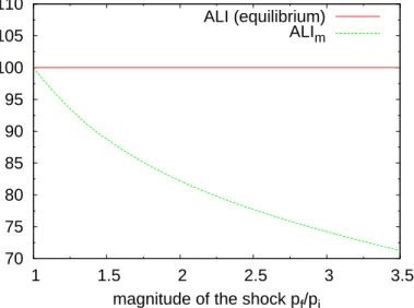
Fig. 5. The Aggregate Landowners’ Income with respect to the magnitude of changes in transportation prices (index ALIi = ALIf = 100), before and after the shock.
portation price, will be a situation in which more housing is concentrated close to the CBD and less far from it. This transitory ill-adaptation of housing sup-ply makes aggregated housing rents be lower during the medium run than over the long run: AHRm < AHRf. Thus, landowners, as a group, see their
situation deteriorate during the adaptation process, while they are insensitive to transportation price over the long run.
Therefore, the aggregate land income ALI, which is insensitive to transporta-tion costs in a CSEn, depends on this price in a CSEx: Figure 5 shows that the aggregate income of landowners during the transition is always lower than the land income in a CSEn (initial and final periods). For example, a dou-bling of transportation price decreases ALI by approximately 17 percent in the medium run.
Individual effects
Inside the landowners’ group, situations are very diverse. Indeed, because buildings are not adjusted to rents any more, the local return on equity of their investments in buildings depends on the distance r from the CBD, which is not the case in a CSEn. Thus, some investments will reveal more profitable than initially planned, while others will reveal less profitable.
Figure 6 shows the rent with respect to the distance from CBD, during the ini-tial (RHi(p, r)), medium (RHm(2p, r)) and final (RHf(2p, r)) periods. Because
of inertia, the housing rent earned by landowners is slightly higher during the medium-run than in the final stage close to the CBD, but is lower in most of the city’s locations.
0 0.5 1 1.5 2 2.5 0 5 10 15 20 25 30 35 40 45 distance from CBD RHi(p,r) RHm(2p,r) RHf(2p,r)
Fig. 6. The housing rent during the three periods, for a shock corresponding to a doubling of the transportation price (index RH(p, 0) = 1).
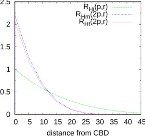
0 0.5 1 1.5 2 2.5 3 3.5 4 0 5 10 15 20 25 30 35 40 45 distance from CBD LLIi(p,r) LLIm(2p,r) LLIf(2p,r) -0.5 0 0.5 1 1.5 2 2.5 0 5 10 15 20 25 30 35 40 45 distance from CBD Land(r).LLIi(p,r) Land(r).LLIm(2p,r) Land(r).LLIf(2p,r)
Fig. 7. Left: for a doubling of the transportation price, the income generated by land with respect to the location r, in the three periods (index LLI(p, 0) = 1). Right: for the same shock, the landowners’ income generated by the entire surface at distance r from CBD (index Land(5) · LLIi(5) = 1).
The effects on the income generated by land LLI(r) is significant, as illus-trated by Fig. 7, which shows the income per unit of land (LLI) and the total land income as a function of the distance from the CBD8. Indeed, two
processes make the medium-period LLIm(r) differ from its final-period value
LLIf(r) (see Eq. (16)): (i) the amount of installed capital K (or, equivalently,
x∗) is different since, only in the final stage, landowners have adjusted their
investments. Capital costs ρK are, therefore, also different. (ii) The rents RH
are different, as a direct consequence of the change in available housing supply. The consequences of these complex interactions are the following. First, close
8 This total land income accounts for the fact that much more land is available far
to the CBD, between a distance zero and 15 km, these processes compen-sate for each others, and the land income during the medium period is only slightly superior than or equal to its long-run value, and much larger than its initial-period value. But, at the outskirts of the city, rents have fallen, while investments remain at a relatively high level, incurring larger capital costs. Thus, LLIm(r) gets there lower than its values at the initial and final period,
and is even negative for distance larger than 20 km. And because land is more and more abundant as distance r increases, those losses in land incomes have a strong impact on aggregate figures.
The right side of Fig. 7 shows the total income generated at a given distance from the CBD, i.e. the amount of available land at a given distance multiplied by the income per unit of land at this location. This figure shows more clearly the large increase in income close to the CBD and the large loss of income far from the CBD. At the aggregate level, losses are greater than gains and ALIm
is lower than ALIf, as illustrated by Fig. 5.
3.2.2 Impacts on households
We saw in Section 3.1 that an increase in transportation prices unambiguously decreases utility in the long run: uf < ui. Nevertheless, buildings inertia can,
over the medium run, either smooth or amplify the negative impact of a shock on transportation prices.
Indeed, this medium-term utility level um depends on the new, increased
trans-portation price and on the inherited housing structure. Compared to this, uf
depends on the same, new, transportation price, and on a new, endogenous housing structure, adapted to this price. For households, the effect of this in-herited housing structure are ambiguous compared with the final situation. On the one hand, the amount of housing close to the CBD is lower during the medium period than at equilibrium, driving um downward compared with uf;
but on the other hand, the amount of housing far from the CBD is larger than at equilibrium, driving um upward. As there is more land available at those
locations, the latter effect may prove significant.
It is hard to predict how these two effects will be balanced. We can get insights on this question by noticing that analytically (computations can be found in Appendix), the endogenous housing structure for j ∈ {i, f } is given by:
Hj(r) = ˜Ar ³
p2j(Y − pjr)γ+1 ´b
(22)
using µ = pf/pi as an indicator of the price increase, we note that: Hf(r) > Hi(r) ⇔ r < Y pi µ2aβ − 1 µ2aβ+1− 1 (23) and that: Hf(r) Hi(r) =hµ2/(γ+1)Y /pi− µr Y /pi− r ib(γ+1) (24)
This ratio depends on the scope of the price increase µ as well as on the initial level of the transportation price pi. One can easily check that, for any given
initial price level pi, the city will concentrate towards the center. Therefore, at
locations far from the center, Hi(r) > Hf(r). The opposite happens close to
the CBD (see Fig. 2a). We can define a location r(µ) at which Hi(r) = Hf(r).
As µ gets stronger, r gets closer to the CBD, and the two effects we mentioned get stronger. Also, the lower was the initial price pi, the larger is Hf(r)/Hi(r)
at all r, and the larger are the two effects.
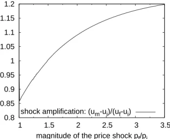
Numerically, the model shows that the larger the relative amplitude of the price shock, the stronger is the negative impact of inertia on households. As a consequence, for a given absolute transportation price increase, cities adapted to low transportation prices are more vulnerable than those already adapted to high transportation prices.
Indeed, the greater µ = pf/pi, the higher is (um − ui)/(uf − ui). This can
be seen in Fig. 8, which shows that the utility shock is smoothened on the medium-term timescale when the magnitude of the transportation price shock is small (µ ≤ 1.6), and amplified otherwise.
This property is explained by the fact that, during the medium period, demand by households is flexible, while supply by landowners is rigid. This asymmetry (i) allows households to capture a transfer of wealth from the landowners who own land far from the CBD; and (ii) leads to a lack of housing supply close to the CBD, which creates a scarcity rent for landowners who own land there. The stronger is the shock, however, the larger is the former effect and the weaker is the latter (since households devote more money to transportation). Combined, these effects cause a positive transfer of wealth from landowners to households, which strengthens as the shock gets stronger, as can be seen from the response of ALI (see Fig. 5).
For moderate shocks, the transfer of wealth dominates the utility losses due to the suboptimality of housing supply, and buildings inertia reduces households utility losses by up to 14 percent. For large shocks (µ > 1.6), on the other
0.8 0.85 0.9 0.95 1 1.05 1.1 1.15 1.2 1 1.5 2 2.5 3 3.5
magnitude of the price shock pf/pi shock amplification: (um-ui)/(uf-ui)
Fig. 8. Effect of buildings inertia on the medium-period utility - for shock am-plitude lower than 1.6, the medium-period utility is larger than the final-period utility and housing inertia smoothes the shock; for shock amplitude larger than 1.6, the medium-period utility is lower than the final-period utility and housing inertia amplifies the shock, by up to 20% for the largest increase we investigated.
hand, inertia amplifies utility losses by up to 20 percent. In this case, the wealth transfer from landowners to households cannot compensate for the medium-term lack of housing supply close to the CBD.
4 Conclusion
This paper illustrates the fact that changes in households behavior can reduce the adverse consequences of a sudden increase in transportation costs, but that inertia in buildings and city structures significantly increase the vulnerability to such an event. And, as we are considering generalized transportation costs, such a shock on prices can be induced either by an increase in energy cost, by the introduction of a carbon tax, or by a decrease in transportation speed due to changes in urban planning or to climate policies aiming at decreasing aggregate transportation use (as proposed, for example, by Fergusson (2003)).
To study the effects of behavioral changes and buildings inertia, we have pro-posed a theoretical framework suited for the analysis of a change in urban transport characteristics and we have used numerical simulations to produce transitions between long-term equilibria associated with different transporta-tion costs.
After a doubling of transportation costs, for instance, our model predicts that the adjustment of households housing and localization choices can largely
re-duce the adverse consequences of the shock. Unsurprisingly, this result shows that assessing the consequences of a price shock using an unchanged con-sumption bundle, i.e. assuming an inelastic transportation demand, leads to a strong overestimation of its adverse effects in the long run.
However, even after these adjustments, buildings inertia is responsible, during a long transitory period, for a suboptimality in housing supply and a transfer of wealth from landowners to households. The combination of these effects has significant adverse consequences: (i) a 17-percent decrease in land income for the landowners as a group, while this income is insensitive to transportation costs at equilibrium, i.e. when landowners have adjusted their investments and, therefore, the supply in housing services; (ii) a large redistribution of wealth among landowners, with enormous losses for those who own land far from the center; and (iii) a 9-percent amplification of household’s utility losses, compared with the same shock without buildings inertia. We also found that the greater the shock, the more important is the negative influence of inertia on medium-term utility and landowners’ income.
Overall, the consequences of buildings inertia are far from negligible and they suggest that a high (even low-frequency) variability in energy or transportation costs, which makes it impossible for the slowly-evolving urban structure to be optimal at each point in time, can cause large welfare and economic losses. Reducing energy price variability may, therefore, be a worthy policy objective. As we suggested in the introduction, these results also show that buildings inertia is a major parameter to account for in the design and assessment of energy policies.
For example, the mechanisms highlighted in this paper would influence the efficiency cost of a carbon tax, but are not taken into account yet in the pub-lished assessments of mitigation economic costs (e.g., Jorgenson et al., 1992; Edenhofer et al., 2006), even those that model explicitly households trans-portation choices (Crassous et al., 2006). Obviously, assuming that a long-term increase in energy and transportation prices is unavoidable, because of resource scarcity and climate change, the inertia of the built environment calls for specific implementations of energy policies. Adequate implementa-tion paths would start as soon as possible, and be smooth but immediately significant. Thus, they would induce an immediate taking into account of fu-ture energy prices in buildings design and urban strucfu-tures, without causing large utility losses over the medium-term.
Also, in the numerous fast-growing cities of the developing world, the urban structure and transportation infrastructure will be, to a large extent, designed and built in the coming decades. Our results call for the immediate implemen-tation of ambitious transporimplemen-tation and urban policies that limit urban sprawl, to reduce the vulnerability of these cities to the likely future increase in
trans-portation costs.
Finally, the heterogeneity of the consequences of the price change — between landowners and households and among landowners — shows that aggregate estimates of energy-policy outcomes must be used with caution, since limited aggregate effects can hide significant consequences for some categories.
As it is, our model is able to demonstrate that households behaviors and buildings inertia are important processes that must be taken into account in the design and evaluation of energy policies. However, further developments of this model, which will be described in follow-up papers, will aim at making it able to produce more detailed assessments. In particular, our first results suggest further developments along three lines.
First, it will be necessary to introduce multiple transportation modes, and the interplay of time constraints and congestion in consumer transportation choices. Second, we assumed that economic agents, including government, did not anticipate the evolutions they would be confronted to, reacting only to current economic signals. Thus, we did not model the implementation of any precautionary measures. In a follow-up paper, we will look at anticipated policies that would allow for a smoothing of the shock. Given the context of large uncertainty, we will focus on policies that improve the robustness and resilience of cities to transportation cost variability. Third, we focused on the medium- and long-term and assumed that housing supply was either perfectly malleable or rigid, depending on the timescale. In further research, we will focus on short-term mechanisms, to model in more details the transition between periods and produce simulations of the continuous evolution of the city structure.
References
Akerman, J., Hojer, M., 2006. How much transport can the climate stand ? — sweden on a sustainable path in 2050. Energy Policy 34, 1944–1957. Alonso, W., 1964. Location and Land Use. Harvard University Press.
Ambrosi, P., Hourcade, J.-C., Hallegatte, S., Lecocq, F., Dumas, P., Ha Duong, M., 2003. Optimal control models and elicitation of attitudes towards cli-mate damages. Environmental Modeling and Assessment 8 (3), 133–147, special issue on ”Modeling the economic response to global climate change. Brueckner, J. K., 2000. Economics of Cities — theoretical perspectives.
Cam-bridge University Press, Ch. 7, pp. 263 – 289.
Brueckner, J. K., Fansler, D. A., 1983. The economics of urban sprawl: The-ory and evidence on the spatial sizes of cities. Review of Economics and Statistics 65, 479–482.
Capozza, D. R., Li, Y., 1994. The intensity and timing of investment: The case of land. The American Economic Review 84.
Crassous, R., Hourcade, J.-C., Sassi, O., 2006. Endogenous structural change and climate targets modeling experiments with Imaclim-R. Energy Journal 27, 259–276.
Edenhofer, O., Lessmann, K., Kemfert, C., Grubb, M., Kohler, J., 2006. In-duced technological change: Exploring its implications for the economics of atmospheric stabilization: Synthesis report from the innovation modeling comparison project. Energy Journal 27, 57–108.
Evans, A. W., 1975. Rent and housing in the theory of urban growth. Journal of Regional Science 15, 113–25.
Fergusson, M., 2003. The effect of vehicle speeds on emissions. Energy Policy 22 (2), 103–106.
Fisch, O., 1977. Dynamics of the housing market. Journal of Urban Economics 4, 428–77.
Greenwood, J., Hercowitz, Z., 1991. The allocation of capital and time over the business cycle. Journal of Political Economy 99, 1188–1214.
Hourcade, J.-C., Robinson, J., 1996. Mitigating factors: assessing the costs of reducing GHG emissions. Energy Policy 24, 863–873.
Jin, Y., Zeng, Z., 2004. Residential investment and house prices in a multi-sector monetary business cycle model. Journal of Housing Economics 13, 268–286.
Jorgenson, D. W., Slesnick, D. T., Wilcoxen, P. J., Joskow, P. I., Kopp, R., 1992. Carbon taxes and economic welfare. Brookings Papers on Economic Activity, Microeconomics 1992, 393–454.
McGrath, D. T., 2005. More evidence on the spatial scale of cities. Journal of Urban Economics 58, 1–10.
Mills, S. E., 1967. An aggregative model of resource allocation in a metropoli-tan area. The American Economic Review 57 (2), 197–210, papers and Pro-ceedings of the Seventy-ninth Annual Meeting of the American Economic Association.
Muth, R. F., 1969. Cities and Housing — The Spatial Pattern of Urban Res-idential Land Use. The University of Chicago Press.
Noland, R. B., Cowart, W. A., Fulton, L. M., 2006. Travel demand policies for saving oil during a supply emergency. Energy PolicyIn press.
O’Toole, R., 2003. Transportation costs and the american dream. Special re-port, Surface Transportation Policy Project.
Reschovsky, C., 2004. Journey-to-work: 2000. Census 2000 brief, U.S. Census Bureau.
Von Thuenen, J. H., 1826. Der Isolierte Staat in Beziehung auf Landwirtschaft und Nationaloekonomie. Perthes.
Weyant, J. P., 1993. Costs of reducing global carbon emissions. The Journal of Economic Perspectives 7 (4), 27–46.
Yacovissi, W., Kern, C. R., 1995. Location and history as determinants of urban residential density. Journal of Urban Economics 38, 207–220.
5 Appendix: analytical calculations
5.1 Long-term equilibrium with endogenous housing structure
5.1.1 Characteristics of the urban system
Setting γ = aβ1 − 1 and B = (Ab)1/a(ααββ)1/aβ a
bρb/a, the solutions of the
equilibrium problem satisfy:
RH(r, u) = ³ ααββ Y −pr u ´1/β s(r, u) = B(γ+1)uγ+1 [Y − pr]−γ rf(u) = Y /p (25)
Concerning the endogenous housing structure, it comes:
k(r, u) = bβρb/a(Y − pr) k s(r, u) = b aρb/aB[Y − pr]γ+1u−(γ+1) H(r, u) = lrA³b aρ b/aB[Y − pr]γ+1u−(γ+1)´b (26) 5.1.2 Utility level
Equation (8) on the city population implies:
N = rf Z 0 L(r) s(r, u)dr = rf Z 0 lrB(γ + 1)[Y − pr]γu−(γ+1)dr
This equation gives us the relation: p2N lB = −Y RA B + u ³RA B ´γ+1γ+2γ + 1 γ + 2 + u −(γ+1)Yγ+2 γ + 2 (27)
Right Hand Side of Eq. (27) is strictly decreasing with u as soon as u is such that rf can be positive. The interpretation of the decrease of RHS of Eq. (27)
with u is that, ceteris paribus, an increase in u implies that N shall decrease, i.e. some people shall leave the city.
5.1.3 Housing structure
H(r) = n(r)q(r) = lrF (1, k(r)/s(r)).
Using Eq. (25), we have then:
H(r) = A0 lr³bβ(γ + 1)(γ + 2)N l (p)( Y p) −(γ+2) (Y p − r) γ+1´b (28) where A0 = Ab (1−ρ)
Furthermore, we can compute landowners’ profits per square meter of land, depending on the location of the land:
LLI(r) = H(r) · RH(r) − ρLand(r) · ks(r) will give us:
LLI(r) = N (γ + 2) l (p) ³Y p ´−(γ+2)³Y p − r ´γ+1 (29) 5.2 Nomenclature
r distance from CBD α utility function q housing service per household β utility function s land area per household Ra agricultural land rent
k capital per household RH unit housing service rent
z composite good a construction function L land surface b construction function
K capital i initial period
T transportation costs f final period
p transportation price per km m medium-term equilibrium Y income per capita rf city frontier
H housing service density per unit of land surface l density of land ψ bid-rent function n density of households θ discount factor
u utility level U utility function