When Can Inverted Water Tables Occur Beneath
Streams?
by Yueqing Xie
1, Peter G. Cook
2,3, Philip Brunner
4, Dylan J. Irvine
2, and Craig T. Simmons
2Abstract
Decline in regional water tables (RWT) can cause losing streams to disconnect from underlying aquifers. When this occurs, an inverted water table (IWT) will develop beneath the stream, and an unsaturated zone will be present between the IWT and the RWT. The IWT marks the base of the saturated zone beneath the stream. Although a few prior studies have suggested the likelihood of an IWT without a clogging layer, most of them have assumed that a low-permeability streambed is required to reduce infiltration from surface water to groundwater, and that the IWT only occurs at the bottom of the low-permeability layer. In this study, we use numerical simulations to show that the development of an IWT beneath an unclogged stream is theoretically possible under steady-state conditions. For a stream width of 1 m above a homogeneous and isotropic sand aquifer with a 47 m deep RWT (measured in an observation point 20 m away from the center of the stream), an IWT will occur provided that the stream depth is less than a critical value of 4.1 m. This critical stream depth is the maximum water depth in the stream to maintain the occurrence of an IWT. The critical stream depth decreases with stream width. For a stream width of 6 m, the critical stream depth is only 1 mm. Thus while theoretically possible, an IWT is unlikely to occur at steady state without a clogging layer, unless a stream is very narrow or shallow and the RWT is very deep.
Introduction
The growing water demand in recent years has caused increased exploitation of groundwater and widespread declines in regional water tables (RWT). As the water table declines, streams that are initially receiving ground-water (gaining streams) may change into losing streams (Wilson 1993). As the water table continues to fall, the loss rate from the stream will increase. Eventually, the loss rate will reach a maximum value, and at this point the streams are said to be disconnected from the groundwa-ter system (Sophocleous 2002). Fox and Durnford (2003) and Brunner et al. (2009a, 2009b) have examined this process analytically and numerically. The occurrence of disconnection in a stream-aquifer system is characterized by the development of an inverted water table (IWT). 1Corresponding author: National Centre for Groundwater
Research and Training, School of the Environment, Flinders University, Adelaide, South Australia, Australia; 61882015140; fax: 61882017906; yueqing.xie@flinders.edu.au
2National Centre for Groundwater Research and Training,
School of the Environment, Flinders University, Adelaide, South Australia, Australia.
3Water for a Healthy Country National Research Flagship,
Division of Land and Water, Commonwealth Scientific and Industrial Research Organization, Adelaide, South Australia, Australia.
4Centre d’Hydrog´eologie et de G´eothermie, University of
Neuchˆatel, Neuchatel, Switzerland.
The IWT is the boundary of the saturated zone immedi-ately underneath the stream as shown in Figure 1. The pressure at the IWT is equal to atmospheric pressure. The term IWT is also used to describe the bottom of the satu-rated part in a perched aquifer (Freeze and Cherry 1979) and the transient front of infiltration after intensive rain-fall or managed surface ponding (Gerla 1992; Racz et al. 2012). Here we use the term IWT to define the base of the saturated zone underneath the stream.
Several studies have investigated stream-aquifer dis-connection with a clogging layer (i.e., a low-permeability streambed). This clogging layer can cause significant head loss (Fox and Durnford 2003) and result in a disconnec-tion regime under certain circumstances. Brunner et al. (2009a) derived a one-dimensional criterion to quantify whether a stream-aquifer system can become fully dis-connected with the presence of a clogging layer.
Streams may not always develop clogging layers. In streams with fast moving water, for example, fine-grained sediments cannot deposit and settle to form less conductive streambeds (Peterson and Wilson 1988). It is clear that an IWT can develop under transient conditions in the absence of a clogging layer. In fact, this will always be the case after the commencement of flow in a previously dry, ephemeral stream. However, of more interest is whether an IWT can continue to exist under steady-state conditions. Prior studies (Fox and Durnford 2003; Bruen and Osman 2004) implied that a clogging layer is necessary for disconnection to occur at steady
Published in Groundwater, Vol. 52, Issue 5, 2014, p. 769-774
Figure 1. Geometry and boundary conditions of the model domain. The hydraulic head boundary condition in the top left represents the stream. Another hydraulic head boundary condition is placed at the lower part of the right-hand side to represent regional groundwater. All other boundary conditions are no flow.
state. However, lab experiments (Day and Luthin 1954; Wang et al. 2011) and early-stage numerical models (Reisenauer 1963) have shown disconnected regimes and IWTs without clogging layers. Day and Luthin (1954) investigated the steady-state distribution of pressure head under an unlined furrow both mathematically and exper-imentally, and found that most of the soil zone remains unsaturated with an IWT forming at the upper region close to the furrow bottom. Reisenauer (1963) presented numerical modeling results that appear to demonstrate the development of an IWT under a stream, although details of the model setup are not clearly described. In a compre-hensive review on surface water-groundwater interaction, Sophocleous (2002) stated that IWTs can exist under unlined channels with low-lying RWT by citing the study of Reisenauer (1963). Wang et al. (2011) also examined the occurrence of the IWT beneath an unclogged canal in a physical sandbox where they investigated the evolution of connection status of rectangular and triangular streams both with and without clogging layers.
The occurrence of an IWT under an unclogged stream in steady state is attributed to capillarity. Capillary forces create a horizontal hydraulic gradient resulting in a small amount of lateral flow. This widens the flow domain, resulting in less vertical flow per unit area. Provided the
specified dimensions. We then investigated how stream dimensions affect the IWT depth above a deep RWT. All simulations were carried out in steady state.
Numerical Modeling
Numerical experiments were carried out to examine the likelihood of the occurrence of the formation of an IWT between a losing stream and the underlying aquifer under steady-state conditions in the absence of a clogging layer. Due to the need to simulate both saturated and unsaturated flow in this study, the numerical simulator HydroGeoSphere was used (Therrien et al. 2010). The finite difference mode was used throughout this study. The full capabilities of HydroGeoSphere are outlined in a recent review by Brunner and Simmons (2012).
The rectangular model used to represent half of a stream-aquifer system in this study is 50 m deep and 20 m wide. The conceptual model is shown in Figure 1. We deliberately made the aquifer deep in order to maximize the opportunity of reaching disconnection. A hydraulic head boundary condition was assigned to a segment at the left end of the top of the model to represent the water elevation of a steady stream (the sum of stream depth and the elevation of stream bottom). The stream depth and width were varied systematically to examine variation in the state of connection in response to the change of the stream condition. Note that with our model setup lateral flow cannot occur from stream sides. Another hydraulic head boundary condition was assigned to a segment of the right-hand side boundary, extending from the bottom end upwards to represent regional groundwater. This boundary condition allows the drainage of groundwater and therefore avoids fill-up of the domain. The model was discretized uniformly with elemental sizes of 0.1 m both horizontally and vertically. The selection of this grid discretization was carefully carried out by ensuring no significant difference between the current grid scheme and the finer one. All models were simulated in steady state.
We assume the sand aquifer in this study is homoge-neous and isotropic. In our simulations, typical saturated hydraulic conductivity (K= 1 m/d) and van Genuchten
Figure 2. The steady-state saturation distribution in a sand aquifer with the water table at the right-hand side boundary lowered by (a) 3 m, (b) 12 m, (c) 18.5 m, (d) 20 m, and (e) 47 m, respectively. Both the stream depth and the width are 1 m.
parameters (α= 14 m−1, β= 2.5) for sand were chosen (Carsel and Parrish 1988).
The development of the IWT was examined in two settings. In the first setting, the stream is 1 m wide and 1 m deep. We examined how the stream disconnects from a sand aquifer by observing the variation in the infiltration rate across the bottom of the stream water body and the variation in the matric head profile, while the RWT (i.e., the head of the lower part of the right-hand side boundary) is systematically lowered from 3 m to 47 m below the land surface. In the second setting, the RWT is fixed at 47 m below the land surface, and we identify the critical stream depth for a given stream width. This critical stream depth is the maximum water depth in the stream to maintain the occurrence of the IWT. A systematic investigation was conducted subsequently to explore the response of the IWT depth to an increase in stream depth for different stream widths.
As the IWT is characterized by the atmospheric pressure (i.e., 0 m matric head), we monitored the variation in the matric head profile. From top, downward underneath the stream, if the matric head at a depth is zero but the matric head underneath is nonzero, this depth is treated as the IWT. The RWT can also be identified in a similar manner. The region between the IWT and the RWT is the unsaturated zone. The air entry value is not included in this study. Hence, when pressure drops below zero, an unsaturated zone develops.
Results
The Occurrence of an IWT
We demonstrate the development of an IWT by visually inspecting the change of saturation distribution in response to the progressive drop of the RWT while the
width and the depth of the stream are fixed, as shown in Figure 2. It is evident that when the water table is shallow (high value of hydraulic head at the right-hand side boundary), the stream is entirely connected to groundwater because lateral capillary forces are not sufficiently strong to widen the flow domain before the infiltrating water reaches the RWT. While the RWT is progressively lowered, the lateral capillary fringe starts to develop. As the RWT is lowered to a depth of around 18.5 m (Figure 2c), lateral flow of water becomes more apparent. Consequently, the infiltrating water is about to be separated from the RWT to form an IWT beneath the stream and a groundwater mound underneath with an unsaturated zone in between.
The RWT depth at which disconnection first occurs is then quantified by examining both the variation in the infiltration rate and the change of the matric head profile as shown in Figure 3. Figure 3a shows that the infiltration rate increases rapidly from 1.1 m/d to 2.4 m/d when the RWT is lowered from a depth of 3 m to around 12 m, and asymptotically approaches a value of 2.42 m/d as the RWT is lowered further. When the RWT is lowered below a depth of 18.5 m, an unsaturated zone develops as indicated by the matric head profile (red line and red solid circles in Figure 3b). Further lowering of the RWT does not affect the depth of the IWT suggested by the top of the matric head profile. However, the distance between the IWT and the groundwater mound increases. This depth of 18.5 m marks the change from connection to disconnection as indicated by the dashed line in Figure 3a. It is clear from Figure 3a that the infiltration rate is no longer dependent on the RWT depth.
We must highlight that the size and the outline of the saturated zone in between the stream and the IWT no longer vary once the stream disconnects at a RWT depth below 18.5 m. Hence, there is no further variation in
the stream (i.e., at x= 0 m) between the stream bottom and the base of the aquifer for four depths of the RWT. Matric head of 0 m in (b) indicates full saturation.
infiltration rate because of unchanged hydraulic gradient between the bottom of the stream and the IWT. However, it is also worth noting that the matric heads in the unsaturated zone are very close to zero, and so the presence of the unsaturated zone would be difficult to detect using field methods.
The Effect of Stream Width and Depth
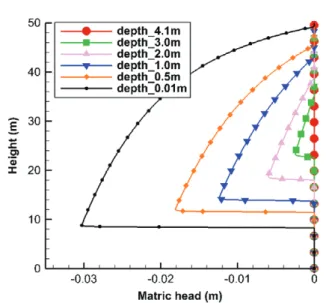
If the aquifer hydraulic parameters are fixed, then the location of the IWT above a deep RWT is determined only by the dimensions of the overlying stream. Figure 4 depicts matric head profiles beneath the stream (i.e., at x= 0 m) for stream width of 1 m and a range of stream depths. As we move upwards from the base of the aquifer towards the surface, a rapid decrease in the matric head marks the position of the RWT beneath the stream. Above this point, the matric head gradually increases, and approaches 0 m at the base of the IWT. The unsaturated zone between the RWT and the IWT reduces with the increase in the stream depth, due to the increase in infiltration rate. Once the stream depth exceeds a value of 4.1 m, negative matric head cannot be detected and hence the whole region below the stream is fully saturated. This stream depth is the critical depth at which point the stream-aquifer system changes from disconnected to connected for this specific hydrogeologic setting. It should also be noted that for any stream depth less than 4.1 m, the position of the IWT is independent of the position of the RWT.
Using this approach, the relationship between the critical stream depth and the stream width, can be derived (Figure 5). In theory, any combination of stream depth and width located above the curve in Figure 5 will remain fully connected to the RWT for a homogeneous and isotropic sand aquifer at all times. Wide streams require a smaller water depth to maintain the connection between the stream and the aquifer. This is because for a wide infiltrating water body, the lateral water flow rate is small relative to the downward flow rate. For this specific RWT depth
Figure 4. The evolution of the matric head profile beneath the stream (i.e., at x= 0 m) with the change of stream depth at stream width of 1.0 m in a sand aquifer. The RWT is fixed at 47 m below the land surface at the right-hand side boundary of the model domain.
at 47 m, the stream never disconnects once its width is greater than around 6 m, provided the stream has a minimum depth of 1 mm.
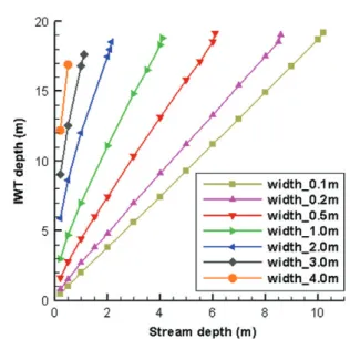
Figure 6 demonstrates the variation in the depth of the IWT with stream depth at various fixed stream widths. These curves were generated with the RWT at the right-hand side boundary set at 47 m. For any fixed stream width, the relationship between the IWT depth and the stream depth is approximately linear. The upper end of each curve indicates the maximum depth of the IWT. Clearly, an IWT will occur and the stream-aquifer system will be disconnected, provided the depth of the regional water table directly under the stream is less than the IWT depth given by this figure. For deeper RWTs, these curves are unchanged, but upper ends are extended following the trends as deeper streams and hence greater IWT depths
Figure 5. The relationship between stream width and critical stream depth, below which disconnection can occur. Stream does not disconnect when the combination of stream depth and width is above the curve. The RWT is set at a depth of 47 m at the right-hand side boundary of the model domain.
Figure 6. Relationship between the IWT depth and the stream depth at various stream widths. The upper end of each curve indicates the maximum depth of the IWT for a specific stream width.
are allowed to maintain disconnection. Of course, these curves will change depending on the hydraulic properties of the aquifer material.
Figure 7 compares the variation in the IWT depth with the stream depth for three different sediment types. The stream widths for all cases are fixed at 1.0 m and the RWTs are 47 m deep beneath the land surface. It is shown that the relationship between the IWT depth and the stream depth varies significantly with van Genuchten parameters. As can be seen in Figures 3 and 4, water contents in our simulations are very close to saturation, and so the results would be determined by this part of the retention curve. However, soil water retention equations
Figure 7. Relationship between the IWT depth and the stream depth at the stream width of 1.0 m for three different sediment types. Simulations shown in Figures 1 to 6 use
α= 14.00 m−1, β= 2.50 (Carsel and Parrish 1988), which
represent the hydraulic properties of sand. Other curves represent loam (α= 3.60 m−1, β= 1.56, Carsel and Parrish
1988) and medium sand (α= 9.52 m−1,β= 5.59, Wang et al.
2011). The upper end of each curve indicates the maximum depth of the IWT.
such as van Genuchten are only an approximation, and the shapes of the curves close to saturation are determined by curve-fitting to data. There is rarely (if ever) any field data within the range of matric potentials simulated in this study (i.e.,−0.001 to −0.03 m). Thus while Figure 7 provides some information on how IWT depth varies with water retention parameters, it is difficult to directly relate the different curves to different sediment types.
Discussion
The recent literature on disconnection (Fox and Durn-ford 2003; Bruen and Osman 2004; Brunner et al. 2009a) has implied that disconnection could only occur in the presence of a clogging layer. This is in apparent con-flict with results from an early numerical modeling study (Reisenauer 1963) and a recent sand tank experiment (Wang et al. 2011).
Wang et al. (2011) observed the IWT in the absence of a clogging layer in sand tank experiments where streams were very narrow (around 10 cm). Their exper-imental results show an IWT depth of around 0.3 m. In comparison, our numerical results for sand yield an IWT depth of 0.5 m for the same stream width (width_0.1 m case in Figure 6). This closeness indicates that the occur-rence of an IWT with the small stream width in these experiments is conceivable. However, our attempt to reproduce their IWT numerically was not successful. This may be due to our use of van Genuchten curves which does not accurately represent the sand tank experiment. It may also be related to issues with the sand tank exper-iment, potentially including non steady state, sediment heterogeneity, and entrapped air.
saturation, where there is rarely any data. Nevertheless, our simulations show that it will only occur for very narrow streams and shallow streams overlying very deep RWTs. Thus the statement from Brunner et al. (2009a) that a clogging layer is necessary for disconnection is true for most practical purposes. However, for small drainage channels, this may not apply.
Our analysis was limited to homogeneous and isotropic systems. In practice, many alluvial aquifers are often characterized by strong anisotropy, with horizontal permeability greater than vertical permeability (Freeze and Cherry 1979). Within this study, some preliminary sim-ulations showed that anisotropy increases the likelihood of the occurrence of the IWT and the disconnection due to preferential lateral flow. Wang et al. (2011) conducted simple heterogeneity experiments where a less permeable layer exists at a certain depth below the stream in the aquifer and observed disconnection. The low-permeability layer here acts as a similar barrier to a clogging layer. It is envisaged that when complex heterogeneity is incor-porated into the entire aquifer, both connection and dis-connection are likely to occur under the same stream condition (Frei et al. 2009; Irvine et al. 2012). This aspect also requires further examination.
Conclusions
This study investigated the likelihood of IWTs underneath streams without a low-permeability streambed using a synthetic numerical model. Our results show that IWTs may occur under steady-state conditions. However, although this phenomenon is theoretically possible, it is only likely to occur in very narrow or shallow streams and where RWTs are very deep.
Acknowledgments
This research was funded by National Centre for Groundwater Research and Training, an Australian gov-ernment initiative, supported by the Australian Research
W01422.
Brunner, P., C.T. Simmons, and P.G. Cook. 2009b. Spatial and temporal aspects of the transition from connection to disconnection between rivers, lakes and groundwater. Journal of Hydrology 376, no. 1–2: 159–169.
Carsel, R.F., and R.S. Parrish. 1988. Developing joint probability distributions of soil water retention characteristics. Water Resources Research 24, no. 5: 755–769.
Day, P.R., and J.N. Luthin. 1954. Sand-model experiments on the distribution of water-pressure under an unlined canal. Soil Science Society of America Journal 18, no. 2: 133–136. Fox, G.A., and D.S. Durnford. 2003. Unsaturated hyporheic zone flow in stream/aquifer conjunctive systems. Advances in Water Resources 26, no. 9: 989–1000.
Freeze, R.A., and J.A. Cherry. 1979. Groundwater , 604. Englewood Cliffs, New Jersey: Prentice-Hall, Inc. Frei, S., J.H. Fleckenstein, S.J. Kollet, and R.M. Maxwell.
2009. Patterns and dynamics of river–aquifer exchange with variably-saturated flow using a fully-coupled model. Journal of Hydrology 375, no. 3–4: 383–393.
Gerla, P. 1992. The relationship of water-table changes to the capillary fringe, evapotranspiration, and precipitation in intermittent wetlands. Wetlands 12, no. 2: 91–98. Irvine, D.J., P. Brunner, H.-J.H. Franssen, and C.T. Simmons.
2012. Heterogeneous or homogeneous? Implications of simplifying heterogeneous streambeds in models of losing streams. Journal of Hydrology 424–425: 16–23.
Peterson, D.M., and J.L. Wilson. 1988. Variably saturated flow between streams and aquifers. Tech Completion Rep 233. Socorro: New Mexico Water Resources Research Institute. Racz, A.J., A.T. Fisher, C.M. Schmidt, B.S. Lockwood, and M.L. Huertos. 2012. Spatial and temporal infiltration dynamics during managed aquifer recharge. Ground Water 50, no. 4: 562–570.
Reisenauer, A.E. 1963. Methods for solving problems of multidimensional, partially saturated steady flow in soils. Journal of Geophysical Research 68, no. 20: 5725–5733. Sophocleous, M. 2002. Interactions between groundwater and
surface water: The state of the science. Hydrogeology Journal 10, no. 1: 52–67.
Therrien, R., R.G. McLarren, E.A. Sudicky, and S.M. Panday. 2010. HydroGeoSphere, Groundwater Simulation Group, University of Waterloo, Waterloo, Ontario, Canada. Wang, W., J. Li, X. Feng, X. Chen, and K. Yao. 2011.
Evolution of stream-aquifer hydrologic connectedness dur-ing pumpdur-ing—Experiment. Journal of Hydrology 402, no. 3–4: 401–414.
Wilson, J.L. 1993. Induced infiltration in aquifers with ambient flow. Water Resources Research 29, no. 10: 3503–3512.